∎

Introduction to Decoherence Theory

4.1 The Concept of Decoherence

This introduction to the theory of decoherence is aimed at readers with an interest in the science of quantum information. In that field, one is usually content with simple, abstract descriptions of non-unitary “quantum channels” to account for imperfections in quantum processing tasks. However, in order to justify such models of non-unitary evolution and to understand their limits of applicability it is important to know their physical basis. I will therefore emphasize the dynamic and microscopic origins of the phenomenon of decoherence, and will relate it to concepts from quantum information where applicable, in particular to the theory of quantum measurement.

The study of decoherence, though based at the heart of quantum theory, is a relatively young subject. It was initiated in the 1970’s and 1980’s with the work of H. D. Zeh and W. Zurek on the emergence of classicality in the quantum framework. Until that time the orthodox interpretation of quantum mechanics dominated, with its strict distinction between the classical macroscopic world and the microscopic quantum realm. The mainstream attitude concerning the boundary between the quantum and the classical was that this was a purely philosophical problem, intangible by any physical analysis. This changed with the understanding that there is no need for denying quantum mechanics to hold even macroscopically, if one is only able to understand within the framework of quantum mechanics why the macro-world appears to be classical. For instance, macroscopic objects are found in approximate position eigenstates of their center-of-mass, but never in superpositions of macroscopically distinct positions. The original motivation for the study of decoherence was to explain these effective super-selection rules and the apparent emergence of classicality within quantum theory by appreciating the crucial role played by the environment of a quantum system.

Hence, the relevant theoretical framework for the study of decoherence is the theory of open quantum systems, which treats the effects of an uncontrollable environment on the quantum evolution. Originally developed to incorporate the phenomena of friction and thermalization in the quantum formulation, it has of course a much longer history than decoherence theory. However, we will see that the intuition and approximations developed in the traditional treatments of open quantum systems are not necessarily appropriate to yield a correct description of decoherence effects, which may take place on a time scale much shorter than typical relaxation phenomena. In a sense, one may say that while the traditional treatments of open quantum systems focus on how an environmental “bath” affects the system, the emphasis in decoherence is more on the contrary question, namely how the system affects and disturbs environmental degrees of freedom, thereby revealing information about its state.

The physics of decoherence became very popular in the last decade, mainly due to advances in experimental technology. In a number of experiments the gradual emergence of classical properties in a quantum system could be observed, in agreement with the predictions of decoherence theory. Needles to say, a second important reason for the popularity of decoherence is its relevance for quantum information processing tasks, where the coherence of a relatively large quantum system has to be maintained over a long time.

Parts of these lecture notes are based on the books on decoherence by E. Joos et al. Joos2003a and on open quantum systems by H.-P. Breuer & F. Petruccione Breuer2002a , and on the lecture notes of W. Strunz Strunz2002a . Interpretational aspects, which are not covered here, are discussed in Bacciagaluppi2005a ; Schlosshauer2005a , and useful reviews by W. H. Zurek and J. P. Paz can be found in Zurek2003a ; Paz2001a . This chapter deals exclusively with conventional, i.e. environmental decoherence, as opposed to spontaneous reduction theories Bassi2003a , which aim at  “solving the measurement problem of quantum mechanics” by modifying the Schrödinger equation. These models are conceptually very different from environmental decoherence, though their predictions of super-selection rules are often qualitatively similar.

4.1.1 Decoherence in a Nutshell

Let us start by discussing the basic decoherence effect in a rather general framework. As just mentioned, we need to account for the unavoidable coupling of the quantum system to its environment. Although these environmental degrees of freedom are to be treated quantum mechanically, their state must be taken unobservable for all practical purposes, be it due to their large number or uncontrollable nature. In general, the detailed temporal dynamics induced by the environmental interaction will be very complicated, but one can get an idea of the basic effects by assuming that the interaction is sufficiently short-ranged to admit a description in terms of scattering theory. In this case, only the map between the asymptotically free states before and after the interaction needs to be discussed, thus avoiding a temporal description of the collision dynamics.

Let the quantum state of a system be described by the density operator $\rho$ on the Hilbert space $\mathcal{H}$. We take the system to interact with a single environmental degree of freedom at a time – think of a phonon, a polaron, or a gas particle scattering off your favorite implementation of a quantum register. Moreover, let us assume, for the time being, that this environmental “particle” is in a pure state $\rho_{\text{E}}=|\psi_{\operatorname{in}}\rangle\langle\psi_{\operatorname{in}}|_{\text{E}}$, with $|\psi_{\operatorname{in}}\rangle_{\text{E}}\in\mathcal{H}_{\text{E}}$. The scattering operator $\mathsf{S}_{\operatorname{tot}}$ maps between the in- and out-asymptotes in the total Hilbert space $\mathcal{H}_{\operatorname{tot}}=\mathcal{H}\otimes\mathcal{H}_{E}$, and for sufficiently short-ranged interaction potentials we may identify those with the states before and after the collision. The initially uncorrelated system and environment turn into a joint state,

[before collision] $$\rho_{\operatorname{tot}}=\rho\otimes|\psi_{\operatorname{in}}\rangle\langle\psi_{\operatorname{in}}|_{\text{E}}\;,$$ (4.1)

[after collision] $$\rho^{\prime}_{\operatorname{tot}}=\mathsf{S}_{\operatorname{tot}}[\rho\otimes|\psi_{\operatorname{in}}\rangle\langle\psi_{\operatorname{in}}|_{\text{E}}]\mathsf{S}_{\operatorname{tot}}^{{\dagger}}\;.$$ (4.2)

Now let us assume, in addition, that the interaction is non-invasive with respect to a certain system property. This means that there is a number of distinct system states, such that the environmental scattering off these states causes no transitions in the system. For instance, if these distinguished states correspond to the system being localized at well-defined sites then the environmental particle should induce no hopping between the locations. In the case of elastic scattering, on the other hand, they will be the energy eigenstates. Denoting the set of these mutually orthogonal system states by $\left\{|n\rangle\right\}\in\mathcal{H}$, the requirement of non-invasiveness means that $\mathsf{S}_{\operatorname{tot}}$ commutes with those states, that is, it has the form

$$\mathsf{S}_{\operatorname{tot}}=\sum_{n}|n\rangle\langle n|\,\otimes\mathsf{S}_{n}\;,$$ (4.3)

where the $\mathsf{S}_{n}$ are scattering operators acting in the environmental Hilbert space. The insertion into (4.2) yields

$$\rho^{\prime}_{\operatorname{tot}} = \sum_{m,n}\langle m|\rho|n\rangle|m\rangle\langle n|\otimes\mathsf{S}_{m}|\psi_{\operatorname{in}}\rangle\langle\psi_{\operatorname{in}}|_{\text{E}}\mathsf{S}_{n}^{{\dagger}}$$ (4.4)

$$\equiv \sum_{m,n}\rho_{mn}|m\rangle\langle n|\otimes|\psi_{\operatorname{out}}^{\left(m\right)}\rangle\langle\psi_{\operatorname{out}}^{\left(n\right)}|_{\text{E}}\;,$$

and disregarding the environmental state by performing a partial trace we get the system state after the interaction:

$$\rho^{\prime}=\operatorname{tr}_{\text{E}}\left(\rho_{\operatorname{tot}}^{\prime}\right)=\sum_{m,n}|m\rangle\langle n|\rho_{mn}\underset{\langle\psi_{\text{out}}^{\left(n\right)}|\psi_{\text{out}}^{\left(m\right)}\rangle_{\text{E}}}{\underbrace{\langle\psi_{\operatorname{in}}|\,\mathsf{S}_{n}^{{\dagger}}\mathsf{S}_{m}|\psi_{\operatorname{in}}\rangle_{\text{E}}}}\;.$$ (4.5)

Since the $\mathsf{S}_{n}$ are unitary the diagonal elements, or populations, are indeed unaffected,

$$\rho^{\prime}_{mm}=\rho_{mm}\;,$$ (4.6)

while the off-diagonal elements, or coherences, get multiplied by the overlap of the environmental states scattered off the system states $m$ and $n$,

$$\rho_{mn}^{\prime}=\rho_{mn}\langle\psi_{\text{out}}^{\left(n\right)}|\psi_{\text{out}}^{\left(m\right)}\rangle\;.$$ (4.7)

This factor has a modulus of less than one so that the coherences, which characterize the ability of the system state to display a superposition between $|m\rangle$ and $|n\rangle$, get suppressed. It is important to note that this loss of coherence occurs in a special basis, which is determined only by the scattering operator, i.e. by the type of environmental interaction, and to a degree that is determined by both the environmental state and the interaction.

This loss of the ability to show quantum behavior due to the interaction with an environmental quantum degree of freedom is the basic effect of decoherence. One may view it as due to the arising correlation between the system with the environment. After the interaction the joint quantum state of system and environment is no longer separable, and part of the coherence initially located in the system now resides in the non-local correlation between system and the environmental particle; it is lost once the environment is disregarded. A complementary point of view argues that the interaction constitutes an information transfer from the system to the environment. The more the overlap in (4.7) differs in magnitude from unity, the more an observer could in principle learn about the system state by measuring the environmental particle. Even though this measurement is never made, the complementarity principle then explains that the wave-like interference phenomenon characterized by the coherences vanishes as more information discriminating the distinct, “particle-like” system states is revealed.

To finish the introduction, here is a collection of other characteristics and popular statements about the decoherence phenomenon. One often hears that decoherence (i) can be extremely fast as compared to all other relevant time scales, (ii) that it can be interpreted as an indirect measurement process, a monitoring of the system by the environment, (iii) that it creates dynamically a set of preferred states (“robust states” or “pointer states”) which seemingly do not obey the superposition principle, thus providing the microscopic mechanism for the emergence of effective super-selection rules, and (iv) that it helps to understand the emergence of classicality in a quantum framework. These points will be illustrated in the following, though (iii) has been demonstrated only for very simple model systems and (iv) depends to a fair extent on your favored interpretation of quantum mechanics.

4.1.2 General Scattering Interaction

In the above demonstration of the decoherence effect the choice of the interaction and the environmental state was rather special. Let us therefore now take $\mathsf{S}_{\operatorname{tot}}\operatorname{and}\rho_{\text{E}}$ to be arbitrary and carry out the same analysis. Performing the trace in (4.5) in the eigenbasis of the environmental state, $\rho_{\text{E}}=\sum_{\ell}p_{\ell}|\psi_{\ell}\rangle\langle\psi_{\ell}|\,_{\text{E}}$, we have

$$\rho^{\prime}=\operatorname{tr}_{\text{E}}\left(\mathsf{S}_{\operatorname{tot}}[\rho\otimes\rho_{\text{E}}]\mathsf{S}_{\operatorname{tot}}^{{}^{{\dagger}}}\right) = \sum_{j,\ell}\,p_{\ell}\langle\psi_{j}|\mathsf{S}_{\operatorname{tot}}|\psi_{\ell}\rangle_{\text{E}}\rho\langle\psi_{\ell}|\mathsf{S}^{{\dagger}}_{\operatorname{tot}}|\psi_{j}\rangle_{\text{E}}$$ (4.8)

$$= \sum_{k}\mathsf{W}_{k}\,\rho\mathsf{W}_{k}^{{\dagger}}\;,$$

where the $\langle\psi_{j}|\mathsf{S}_{\operatorname{tot}}|\psi_{\ell}\rangle$ are operators in $\mathcal{H}$. After subsuming the two indices $j,\ell$ into a single one, we get the second line with the Kraus operators $\mathsf{W}_{k}\,$ given by

$$\mathsf{W}_{k} = \sqrt{p_{\ell_{k}}}\langle\psi_{j_{k}}|\mathsf{S}_{\operatorname{tot}}|\psi_{\ell_{k}}\rangle\;.$$ (4.9)

It follows from the unitarity of $\mathsf{S}_{\operatorname{tot}}$ that they satisfy

$$\sum_{k}\mathsf{W}_{k}^{{\dagger}}\mathsf{W}_{k}\,=\mathbbm{I}\;.$$ (4.10)

This implies that (4.8) is the operator-sum representation of a completely positive map $\Phi:\rho\mapsto\rho^{\prime}$ (see Sect. 4.3.1). In other words, the scattering transformation has the form of the most general evolution of a quantum state that is compatible with the rules of quantum theory. In the operational formulation of quantum mechanics this transformation is usually called a quantum operation Kraus1983a , the quantum information community likes to call it a quantum channel. Conversely, given an arbitrary quantum channel, one can also construct a scattering operator $\mathsf{S}_{\operatorname{tot}}$ and an environmental state $\rho_{\text{E}}$ giving rise to the transformation, though it is usually not very helpful from a physical point of view to picture the action of a general, dissipative quantum channel as due to a single scattering event.

4.1.3 Decoherence as an Environmental Monitoring Process

We are now in a position to relate the decoherence of a quantum system to the information it reveals to the environment. Since the formulation is based on the notion of an indirect measurement it is necessary to first collect some aspects of measurement theory Busch1991a ; Holevo2001a .

Elements of General Measurement Theory

Projective Measurements

This is the type of measurement discussed in standard textbooks of quantum mechanics. A projective operator $|\alpha\rangle\langle\alpha|\equiv\mathsf{P}_{\alpha}=\mathsf{P}_{\alpha}^{2}=\mathsf{P}_{\alpha}^{{\dagger}}$ is attributed to each possible outcome $\alpha$ of an idealized measurement apparatus. The probability of the outcome $\alpha$ is obtained by the Born rule

$$\operatorname{Prob}(\alpha|\rho) = \operatorname{tr}\left(\mathsf{P}_{\alpha}\rho\right)=\langle\alpha|\rho|\alpha\rangle\;,$$ (4.11)

and after the measurement of $\alpha$ the state of the quantum system is given by the normalized projection

$$\mathcal{M}:\;\rho \mapsto \mathcal{M}\left(\rho|\alpha\right)=\frac{\mathsf{P}_{\alpha}\rho\mathsf{P}_{\alpha}}{\operatorname{tr}\left(\mathsf{P}_{\alpha}\rho\right)}\;.$$ (4.12)

The basic requirement that the projectors form a resolution of the identity operator,

$$\sum_{\alpha}\mathsf{P}_{\alpha} = \mathbbm{I}\;,$$ (4.13)

ensures the normalization of the corresponding probability distribution $\operatorname{Prob}\left(\alpha|\rho\right)$.

If the measured system property corresponds to a self-adjoint operator $\mathsf{A}$ the $\mathsf{P}_{\alpha}$ are the projectors into its eigenspaces, so that its expectation value is

$$\langle\mathsf{A}\rangle = \operatorname{tr}\left(\mathsf{A}\rho\right)\;.$$

If $\mathsf{A}$ has a continuous spectrum the outcomes are characterized by intervals of a real parameter, and the sum in (4.13) should be replaced by a projector-valued Stieltjes integral $\int\mathrm{d}\mathsf{P}(\alpha)\,\,$=$\mathbbm{I}$, or equivalently by a Lebesgue integral over a projector-valued measure (PVM) Busch1991a ; Holevo2001a .

It is important to note that projective measurements are not the most general type of measurement compatible with the rules of quantum mechanics. In fact, non-destructive measurements of a quantum system are usually not of the projective kind.

Generalized Measurements

In the most general measurement situation, a positive (and therefore hermitian) operator $\mathsf{F}_{\alpha}>0$ is attributed to each outcome $\alpha$. Again, the collection of operators corresponding to all possible outcomes must form a resolution of the identity operator,

$$\sum_{\alpha}\mathsf{F}_{\alpha}\, = \mathbbm{I}.$$ (4.14)

In particular, one speaks of a positive operator-valued measure (POVM) in the case of a continous outcome parameter, $\int\mathrm{d}\mathsf{F}(\alpha)=\mathbbm{I}\,$, and the probability (or probability density in the continuous case) of outcome $\alpha$ is given by

$$\operatorname{Prob}(\alpha|\rho) = \operatorname{tr}\left(\mathsf{F}_{\alpha}\rho\right).$$ (4.15)

The effect on the system state of a generalized measurement is described by a nonlinear transformation

$$\mathcal{M}:\;\rho \mapsto \mathcal{M}\left(\rho|\alpha\right)=\frac{\sum_{k}\mathsf{M}_{\alpha,k}\rho\,\mathsf{M}^{\dagger}_{\alpha,k}}{\operatorname{tr}\left(\mathsf{F}_{\alpha}\rho\right)}$$ (4.16)

involving a norm-decreasing completely positive map in the numerator (see Sect. 4.3.1), and a normalization which is subject to the consistency requirement

$$\sum_{k}\mathsf{M}_{\alpha,k}^{{\dagger}}\mathsf{M}_{\alpha,k} = \mathsf{F}_{\alpha}\,.$$ (4.17)

The operators $\mathsf{M}_{\alpha,k}$ appearing in (4.16) are called measurement operators, and they serve to characterize the measurement process completely. The $\mathsf{F}_{\alpha}$ are sometimes called “effects” or “measurement elements”. Note that different measurement operators $\mathsf{M}_{\alpha,k}$ can lead to the same measurement element $\mathsf{F}_{\alpha}$.

A simple class of generalized measurements are unsharp measurements, where a number of projective operators are lumped together with probabilistic weights in order to account for the finite resolution of a measurement device or for classical noise in its signal processing. However, generalized measurements schemes may also perform tasks which are seemingly impossible with a projective measurement, such as the error-free discrimination of two non-orthogonal states Helstrom1976a ; Chefles2000a .

Efficient Measurements

A generalized measurement is called efficient if there is only a single summand in (4.16) for each outcome $\alpha$,

$$\mathcal{M}\left(\rho|\alpha\right) = \frac{\mathsf{M}_{\alpha}\rho\,\mathsf{M}_{\alpha}^{{\dagger}}}{\operatorname{tr}\left(\mathsf{M}_{\alpha}^{{\dagger}}\mathsf{M}_{\alpha}\rho\right)}\;,$$ (4.18)

implying that pure states are mapped to pure states. In a sense, these are measurements where no unnecessary, that is no classical, uncertainty is introduced during the measurement process, see below. By means of a (left) polar decomposition and the consistency requirement (4.17) efficient measurement operators have the form

$$\mathsf{M}_{\alpha}=\mathsf{U}_{\alpha}\sqrt{\mathsf{F}_{\alpha}}\;,$$ (4.19)

with an unitary operator $\mathsf{U}_{\alpha}$. This way the state after efficient measurement can be expressed in a form which decomposes the transformation into a “raw measurement” described by the $\mathsf{F}_{\alpha}$ and a “measurement back-action” given by the $\mathsf{U}_{\alpha}$:

$$\mathcal{M}\left(\rho|\alpha\right)=\underset{\text{back-action}}{\underbrace{\mathsf{U}_{\alpha}}}\underset{\parbox{50.58878pt}{\centering\scriptsize raw \\ measurement\@add@centering}}{\underbrace{\frac{\sqrt{\mathsf{F}_{\alpha}}\rho\sqrt{\mathsf{F}_{\alpha}}}{\operatorname{tr}\left(\mathsf{F}_{\alpha}\rho\right)}}}\underset{\text{back-action}}{\underbrace{\mathsf{U}_{\alpha}^{{\dagger}}}}\;.$$ (4.20)

In this transformation the positive operators $\sqrt{\mathsf{F}_{\alpha}}$ “squeeze” the state along the measured property and expand it along the other, complementary ones, similar to what a projector would do, while the back-action operators $\mathsf{U}_{\alpha}$ “kick” the state by transforming it in a way that is reversible, in principle, provided the outcome $\alpha$ is known. Note that the projective measurements (4.12) are a sub-class in the set of back-action-free efficient measurements.

Indirect Measurements

In an indirect measurement one tries to obtain information about the system in a way that disturbs it as little as possible. This is done by letting a well-prepared microscopic quantum probe interact with the system. This probe is then measured by projection, i.e. destructively, so that one can infer properties of the system without having it brought into contact with a macroscopic measurement device. Let $\rho_{\text{probe}}$ be the prepared state of the probe, $\mathsf{S}_{\operatorname{tot}}$ describe the interaction between system and probe, and $\mathsf{P}_{\alpha}$ be the projectors corresponding to the various outcomes of the probe measurement. The probability of measuring $\alpha$ is determined by the reduced state of the probe after interaction, i.e.

$$\operatorname{Prob}(\alpha|\rho)=\operatorname{tr}_{\text{probe}}\left(\mathsf{P}_{\alpha}\rho^{\prime}_{\text{probe}}\right)=\operatorname{tr}_{\text{probe}}\left(\mathsf{P}_{\alpha}\operatorname{tr}_{\text{sys}}(\mathsf{S}_{\operatorname{tot}}[\rho\otimes\rho_{\text{probe}}]\mathsf{S}_{\operatorname{tot}}^{{\dagger}})\right)\;.$$ (4.21)

By pulling out the system trace (extending the projectors to ${\mathcal{H}_{\operatorname{tot}}={\mathcal{H}\otimes\mathcal{H}_{\text{p}}}}$) and using the cyclic permutability of operators under the trace we have

$$\operatorname{Prob}(\alpha|\rho)=\operatorname{tr}\left(\mathsf{S}_{\operatorname{tot}}^{{\dagger}}[\mathbbm{I}\otimes\mathsf{P}_{\alpha}]\mathsf{S}_{\operatorname{tot}}\left[\rho\otimes\rho_{\text{probe}}\right]\right)=\operatorname{tr}\left(\mathsf{F}_{\alpha}\rho\right)\;,$$ (4.22)

with microscopically defined measurement elements

$$\mathsf{F}_{\alpha} = \operatorname{tr}_{\text{probe}}\left(\mathsf{S}_{\operatorname{tot}}^{{\dagger}}[\mathbbm{I}\otimes\mathsf{P}_{\alpha}]\mathsf{S}_{\operatorname{tot}}[\mathbbm{I}\otimes\rho_{\text{probe}}]\right)>0$$ (4.23)

satisfying $\sum_{\alpha}\mathsf{F}_{\alpha}=\mathbbm{I}\,.$ Since the probe measurement is projective, we can also specify the new system state conditioned on the click at $\alpha$ of the probe detector,

$$\mathcal{M}\left(\rho|\alpha\right) = \operatorname{tr}_{\text{probe}}\left(\mathcal{M}_{\operatorname{tot}}\left(\rho_{\operatorname{tot}}|\alpha\right)\right)$$ (4.24)

$$= \operatorname{tr}_{\text{probe}}\left(\frac{[\mathbbm{I}\otimes\mathsf{P}_{\alpha}]\mathsf{S}_{\operatorname{tot}}\left[\rho\otimes\rho_{\text{probe}}\right]\mathsf{S}_{\operatorname{tot}}^{{\dagger}}[\mathbbm{I}\otimes\mathsf{P}_{\alpha}]}{\operatorname{tr}\left(\mathsf{F}_{\alpha}\rho\right)}\right)$$

$$= \sum_{k}\frac{\mathsf{M}_{\alpha,k}\rho\mathsf{M}_{\alpha,k}^{{\dagger}}}{\operatorname{tr}\left(\mathsf{F}_{\alpha}\rho\right)}\,\;.$$

In the last step a convex decomposition of the initial probe state into pure states was inserted, $\rho_{\text{probe}}=\sum_{k}w_{k}|\psi_{k}\rangle\langle\psi_{k}|\,$. Taking $\mathsf{P}_{\alpha}=|\alpha\rangle\langle\alpha|$ we thus get a microscopic description also of the measurement operators,

$$\mathsf{M}_{\alpha,k}=\sqrt{w_{k}}\langle\alpha|\mathsf{S}_{\operatorname{tot}}|\psi_{k}\rangle\;.$$ (4.25)

This shows that an indirect measurement is efficient (as defined above) if the probe is initially in a pure state, i.e. if there is no uncertainty introduced in the measurement process, apart from the one imposed by the uncertainty relations on $\rho_{\text{probe}}$.

If we know that an indirect measurement has taken place, but do not know its outcome $\alpha$ we have to resort to a probabilistic (Bayesian) description of the new system state. It is given by the sum over all possible outcomes weighted by their respective probabilities,

$$\rho^{\prime}=\sum_{\alpha}\operatorname{Prob}(\alpha|\rho)\mathcal{M}\left(\rho|\alpha\right)=\sum_{\alpha,k}\mathsf{M}_{\alpha,k}\rho\mathsf{M}_{\alpha,k}^{{\dagger}}\;.$$ (4.26)

This form is the same as above in (4.8) and (4.9), where the basic effect of decoherence has been described. This indicates that the decoherence process can be legitimately viewed as a consequence of the information transfer from the system to the environment. The complementarity principle can then be invoked to understand which particular system properties lose their quantum behavior, namely those complementary to the ones revealed to the environment. This “monitoring interpretation” of the decoherence process will help us below to derive microscopic master equations.

4.1.4 A Few Words on Nomenclature

Since decoherence phenomena show up in quite different sub-communities of physics, a certain confusion and lack of uniformity developed in the terminology. This is exacerbated by the fact that decoherence often reveals itself as a loss of fringe visibility in interference experiments – a phenomenon, though, which may have other causes than decoherence proper. Here is an attempt of clarification:

• decoherence: In the original sense, an environmental quantum effect affecting macroscopically distinct states. The term is nowadays applied to mesoscopically different states as well, and even for microscopic states, as long as it refers to the quantum effect of environmental, i.e. in practice unobservable, degrees of freedom.

  However, the term is often (ab-)used for any other process reducing the purity of a micro-state.

• dephasing: In a narrow sense, this describes the phenomenon that coherences, i.e., the off-diagonal elements of the density matrix, get reduced in a particular basis, namely the energy eigenbasis of the system. It is a statement about the effect, and not the cause. In particular, dephasing may be reversible if it is not due to decoherence, as revealed e.g. in spin-echo experiments.

  This phrase should be treated with great care since it is used differently in various sub-communities. It is taken as a synonym to “dispersion” in molecular physics and in nonlinear optics, as a synonym to “decoherence” in condensed matter, and often as a synonym to “phase averaging” in matter wave optics. It is also called a $T_{2}$-process in NMR and in condensed matter physics (see below).

• phase averaging: A classical noise phenomenon entering through the dependence of the unitary system evolution on external control parameters which fluctuate (parametric average over unitary evolutions). A typical example are the vibrations of an interferometer grating or the fluctuations of the classical magnetic field in an electron interferometer due to technical noise. Empirically, phase averaging is often hard to distinguish from decoherence proper.

• dispersion: Coherent broadening of wave packets during the unitary evolution, e.g. due to a velocity dependent group velocity or non-harmonic energy spacings. This unitary effect may lead to a reduction of signal oscillations, for instance, in molecular pump-probe experiments.

• dissipation: Energy exchange with the environment leading to thermalization. Usually accompanied by decoherence, but see Sect. 4.3.4 for a counter-example.

4.2 Case Study: Dephasing of Qubits

So far, the discussion of the temporal dynamics of the decoherence process was circumvented by using a scattering description. Before going to the general treatment of open quantum systems in Sect. 4.3, it is helpful to take a closer look on the time evolution of a special system where the interaction with a model environment can be treated exactly Palma1996a ; Breuer2002a .

4.2.1 An Exactly Solvable Model

Let us take a two-level system, or qubit, described by the Pauli spin operator $\sigma_{z}$, and model the environment as a collection of bosonic field modes. In practice, such fields can yield an appropriate effective description even if the actual environment looks quite differently, in particular if the environmental coupling is a sum of many small contributions. What is fairly non-generic in the present model is the type of coupling between system and environment, which is taken to commute with the system Hamiltonian.

The total Hamiltonian thus reads

$$\mathsf{H}_{\operatorname{tot}}=\underbrace{\frac{\hbar\omega}{2}\sigma_{z}+\sum_{k}\hbar\omega_{k}\mathsf{b}_{k}^{{\dagger}}\mathsf{b}_{k}}_{\mathsf{H}_{0}}\,+\underset{\mathsf{H}_{\text{int}}}{\underbrace{\sigma_{z}\sum_{k}\left(g_{k}\mathsf{b}_{k}^{{\dagger}}+g_{k}^{\ast}\mathsf{b}_{k}\right)\,}}\;,$$ (4.27)

with the usual commutation relation for the mode operators of the bosonic field modes, $[\mathsf{b}_{i},\mathsf{b}^{{\dagger}}_{k}]=\delta_{ik}$, and coupling constants $g_{k}$. The fact that the system Hamiltonian commutes with the interaction, guarantees that there is no energy exchange between system and environment so that we expect pure dephasing.

By going into the interaction picture one transfers the trivial time evolution generated by $\mathsf{H}_{0\,}$ to the operators (and indicates this with a tilde). In particular,

$$\widetilde{\mathsf{H}}_{\operatorname{int}}\left(t\right)=\mathrm{e}^{{\rm i}\mathsf{H}_{0}t/\hbar}\mathsf{H}_{\operatorname{int}}\mathrm{e}^{-{\rm i}\mathsf{H}_{0}t/\hbar}=\sigma_{z}\sum_{k}(g_{k}\mathrm{e}^{{\rm i}\omega_{k}t}\mathsf{b}_{k}^{{\dagger}}+g_{k}^{\ast}\mathrm{e}^{-{\rm i}\omega_{k}t}\mathsf{b}_{k})\,\;,$$ (4.28)

where the second equality is granted by the commutation $[\sigma_{z},\mathsf{H}_{\operatorname{int}}]=0$. The time evolution due to this Hamiltonian can be formally expressed as a Dyson series,

$$\widetilde{\mathsf{U}}(t) = \mathcal{T}_{\leftarrow}\exp\left(-\frac{{\rm i}}{\hbar}\int_{0}^{t}\mathrm{d}t^{\prime}\widetilde{\mathsf{H}}_{\operatorname{int}}(t^{\prime})\,\right)$$ (4.29)

$$= \sum_{n=0}^{\infty}\,\frac{1}{n!}\left(\frac{1}{{\rm i}\hbar}\right)^{n}\int_{0}^{t}\mathrm{d}t_{1}\cdots\,\mathrm{d}t_{n}\mathcal{T}_{\leftarrow}\left[\widetilde{\mathsf{H}}_{\operatorname{int}}(t_{1})\cdots\widetilde{\mathsf{H}}_{\operatorname{int}}(t_{n})\right]\;,$$

where $\mathcal{T}_{\leftarrow}$ is the time ordering operator (putting the operators with larger time arguments to the left). Due to this time ordering requirement the series usually cannot be evaluated exactly (if it converges at all). However, in the present case the commutator of $\widetilde{\mathsf{H}}_{\operatorname{int}}$ at different times is not an operator, but just a c-number,

$$[\widetilde{\mathsf{H}}_{\operatorname{int}}\left(t\right),\widetilde{\mathsf{H}}_{\operatorname{int}}(t^{\prime})]=2{\rm i}\sum_{k}\left|g_{k}\right|^{2}\sin\left(\,\omega_{k}(t^{\prime}-t)\right)\;.$$ (4.30)

As a consequence, the time evolution differs only by a time-dependent phase from the one obtained by casting the operators in their natural order,

$$\widetilde{\mathsf{U}}(t)=\mathrm{e}^{{\rm i}\varphi(t)}\exp\left(-\frac{{\rm i}}{\hbar}\int_{0}^{t}\mathrm{d}t^{\prime}\widetilde{\mathsf{H}}_{\operatorname{int}}(t^{\prime})\right)\;,$$ (4.31)

where the phase is given by

$$\varphi\left(t\right) = \frac{{\rm i}}{2\hbar^{2}}\int_{0}^{t}\mathrm{d}t_{1}\int_{0}^{t}\mathrm{d}t_{2}\Theta\left(t_{1}-t_{2}\right)\left[\widetilde{\mathsf{H}}_{\operatorname{int}}\,\left(t_{1}\right),\widetilde{\mathsf{H}}_{\operatorname{int}}\,\left(t_{2}\right)\right]\;.$$ (4.32)

One can now perform the integral over the interaction Hamiltonian to get

$$\widetilde{\mathsf{U}}(t)=\mathrm{e}^{{\rm i}\varphi(t)}\exp\left(\frac{1}{2}\sigma_{z}\sum_{k}\left(\alpha_{k}(t)\mathsf{b}_{k}^{{\dagger}}-\alpha_{k}^{\ast}(t)\mathsf{b}_{k}\right)\,\right)\;,$$ (4.33)

with complex, time-dependent functions

$$\alpha_{k}(t):=2g_{k}\frac{1-\mathrm{e}^{{\rm i}\omega_{k}t}}{\hbar\omega_{k}}\;.$$ (4.34)

The operator $\widetilde{\mathsf{U}}(t)$ is diagonal in the eigenbasis of the system, and it describes how the environmental dynamics depends on the state of the system. In particular, if the system is initially in the upper level, $|\psi\rangle=|\uparrow\rangle$, one has

$$\widetilde{\mathsf{U}}(t)|\uparrow\rangle|\xi_{0}\rangle_{\text{E}}=\mathrm{e}^{{\rm i}\varphi(t)}|\uparrow\rangle\prod_{k}\mathsf{D}_{k}\left(\frac{\alpha_{k}(t)}{2}\right)|\xi_{0}\rangle\hskip 6.00006pt=:\mathrm{e}^{{\rm i}\varphi(t)}|\uparrow\rangle|\xi_{\uparrow}\left(t\right)\rangle_{\text{E}}\;,$$ (4.35)

and for the lower state

$$\widetilde{\mathsf{U}}(t)|\downarrow\rangle|\xi_{0}\rangle_{\text{E}}=\mathrm{e}^{{\rm i}\varphi(t)}|\downarrow\rangle\prod_{k}\mathsf{D}_{k}\left(-\frac{\alpha_{k}(t)}{2}\right)|\xi_{0}\rangle\hskip 6.00006pt=:\hskip 6.00006pt\mathrm{e}^{{\rm i}\varphi(t)}|\downarrow\rangle|\xi_{\downarrow}\left(t\right)\rangle_{\text{E}}\;.$$ (4.36)

Here we introduced the unitary displacement operators for the $k$-th field mode,

$$\mathsf{D}_{k}(\alpha) = \exp(\alpha\mathsf{b}^{{\dagger}}_{k}-\alpha^{\ast}\mathsf{b}_{k})\;,$$ (4.37)

which effect a translation of the field state in its attributed phase space. In particular, the coherent state $|\alpha\rangle_{k}$ of the field mode $k$ is obtained from its ground state $|0\rangle_{k}$ by ${|\alpha\rangle_{k}:=\mathsf{D}_{k}(\alpha)|0\rangle_{k}}$ Walls1994a .

The equations (4.35) and (4.36) show that the collective state of the field modes gets displaced by the interaction with the system and that the sense of the displacement is determined by the system state.

Assuming that the states of system and environment are initially uncorrelated, $\rho_{\operatorname{tot}}\left(0\right)=\rho\otimes\rho_{\text{E}},$ the time-evolved system state reads

$$\tilde{\rho}(t)=\operatorname{tr}_{\text{E}}\left(\widetilde{\mathsf{U}}(t)[\rho\otimes\rho_{\text{E}}]\widetilde{\mathsf{U}}^{{\dagger}}(t)\right)\;.$$ (4.38)

It follows from (4.35) and (4.36) that the populations are unaffected,

$$\langle\uparrow|\tilde{\rho}(t)|\uparrow\rangle = \langle\uparrow|\tilde{\rho}(0)|\uparrow\rangle\;,$$

$$\langle\downarrow|\tilde{\rho}(t)|\downarrow\rangle = \langle\downarrow|\tilde{\rho}(0)|\downarrow\rangle\;,$$

while the coherences are suppressed by a factor which is given by the trace over the displaced initial field state,

$$\langle\uparrow|\tilde{\rho}(t)|\downarrow\rangle=\langle\uparrow|\tilde{\rho}(0)|\downarrow\rangle\underbrace{\operatorname{tr}_{\text{E}}\left(\prod_{k}\mathsf{D}_{k}(\alpha_{k}(t))\rho_{\text{E}}\,\right)}_{\chi\left(t\right)}\;.$$ (4.39)

Incidentally, the complex suppression factor $\chi\left(t\right)$ is equal to the Wigner characteristic function of the original environmental state at the points $\alpha_{k}(t)$, i.e. it is given by the Fourier transform of its Wigner function Hillery1984a .

Initial Vacuum State

If the environment is initially in its vacuum state, $\rho_{\text{E}}=\bigotimes_{k}\,|0\rangle\langle 0|_{k}$, the $|\xi_{\uparrow}\left(t\right)\rangle_{\text{E}}$  and $|\xi_{\downarrow}(t)\rangle_{\text{E}}$ defined in (4.35), (4.36) turn into multi-mode coherent states, and the suppression factor can be calculated immediately to yield:

$$\chi_{\operatorname{vac}}(t) = \prod_{k}\langle 0|\mathsf{D}_{k}(\alpha_{k}(t))|0\rangle_{k}\,=\prod_{k}\exp\left(-\frac{\left|\alpha_{k}(t)\right|^{2}}{2}\right)$$ (4.40)

$$= \exp\left(-\sum_{k}4\left|g_{k}\right|^{2}\frac{1-\cos\left(\omega_{k}t\right)}{\hbar^{2}\omega_{k}^{2}}\,\right)\,\;.$$

For times that are short compared to the field dynamics, $t\ll\omega_{k}^{-1}$, one observes a Gaussian decay of the coherences. Modifications to this become relevant at $\omega_{k}t\cong 1$, provided $\chi_{\operatorname{vac}}\left(t\right)$ is then still appreciable, i.e. for $4\left|g_{k}\right|^{2}/\hbar^{2}\omega_{k}^{2}\ll 1$. Being a sum over periodic functions, $\chi_{\operatorname{vac}}(t)$ is quasi-periodic, that is, it will come back arbitrarily close to unity after a large period (which increases exponentially with the number of modes). These somewhat artificial Poincaré recurrences vanish if we replace the sum over the discrete modes by an integral over a continuum with mode density $\mu$,

$$\sum_{k}f(\omega_{k}) \longrightarrow \int_{0}^{\infty}\mathrm{d}\omega\mu(\omega)f(\omega)\;,$$ (4.41)

for any function $f$. This way the coupling constants $g_{k}$ get replaced by the spectral density of the environment,

$$J(\omega) = 4\mu(\omega)\left|g(\omega)\right|^{2}\;.$$ (4.42)

This function characterizes the environment by telling how effective the coupling is at a certain frequency.

Thermal State

If the environment is in a thermal state with temperature $T$,

$$\rho_{\text{E}}=\rho_{\operatorname{th}}=\frac{\mathrm{e}^{-\mathsf{H}_{\text{E}}/k_{B}T}}{\operatorname{tr}\left(\mathrm{e}^{-\mathsf{H}_{\text{E}}/k_{B}T}\right)}=\bigotimes_{k}\underbrace{\left(1-\mathrm{e}^{-\hbar\omega_{k}/k_{B}T}\right)\,\sum_{n=0}^{\infty}\mathrm{e}^{-\hbar\omega_{k}n/k_{B}T}\,|n\rangle\langle n|_{k}}_{=\rho_{\operatorname{th}}^{(k)}}\;,$$ (4.43)

the suppression factor reads

$$\chi(t)=\prod_{k}\operatorname{tr}\left(\mathsf{D}_{k}(\alpha_{k}(t))\rho_{\operatorname{th}}^{(k)}\right)\,=\prod_{k}\exp\left(-\frac{\left|\alpha_{k}(t)\right|^{2}}{2}\coth\left(\frac{\hbar\omega_{k}}{2k_{B}T}\right)\right)\,\;.$$ (4.44)

This factor can be separated into its vacuum component (4.40) and a thermal component, $\chi(t)=\mathrm{e}^{-F_{\operatorname{vac}}(t)}\mathrm{e}^{-F_{\operatorname{th}}(t)}$, with the following definitions of the vacuum and the thermal decay functions:

$$F_{\operatorname{vac}}(t) := \sum_{k}4\left|g_{k}\right|^{2}\frac{1-\cos\left(\omega_{k}t\right)}{\hbar^{2}\omega_{k}^{2}}\;,$$ (4.45)

$$F_{\operatorname{th}}(t) := \sum_{k}4\left|g_{k}\right|^{2}\frac{1-\cos\left(\omega_{k}t\right)}{\hbar^{2}\omega_{k}^{2}}\left(\coth\left(\frac{\hbar\omega_{k}}{2k_{B}T}\right)-1\right)\;.$$ (4.46)

4.2.2 The Continuum Limit

Assuming that the field modes are sufficiently dense we replace their sum by an integration. Noting (4.41), (4.42) we have

$$F_{\operatorname{vac}}(t) \longrightarrow \int_{0}^{\infty}\mathrm{d}\omega J(\omega)\,\frac{1-\cos\left(\omega t\right)}{\hbar^{2}\omega^{2}}$$ (4.47)

$$F_{\operatorname{th}}(t) \longrightarrow \int_{0}^{\infty}\mathrm{d}\omega J(\omega)\,\frac{\left.1-\cos(\omega t\right)}{\hbar^{2}\omega^{2}}\left(\coth\left(\frac{\hbar\omega}{2k_{B}T}\right)-1\right).$$ (4.48)

So far, the treatment was exact. To continue we have to specify the spectral density in the continuum limit. A typical model takes $g\propto\sqrt{\omega}$, so that the spectral density of a $d$-dimensional field can be written as Weiss1999a

$$J(\omega)=a\omega\left(\frac{\omega}{\omega_{c}}\right)^{d-1}\mathrm{e}^{-\omega/\omega_{c}}$$ (4.49)

with “damping strength” $a>0$. Here, $\omega_{c}$ is a characteristic frequency “cutoff” where the coupling decreases rapidly, such as the Debye frequency in the case of phonons.

Ohmic Coupling

For $d=1$ the spectral density (4.49) increases linearly at small $\omega$ (“Ohmic coupling”). One finds

$$F_{\operatorname{vac}}(t)=\frac{a}{2\hbar^{2}}\log(1+\omega_{c}^{2}t^{2})\;,$$ (4.50)

which bears a strong $\omega_{c}$ dependence. Evaluating the second integral requires to assume that the cutoff $\omega_{c}$ is large compared to the thermal energy, $kT\ll\hbar\omega_{c}$:

$$F_{\operatorname{th}}(t)\simeq\frac{a}{\hbar^{2}}\log\left(\frac{\sinh\left(t/t_{\text{T}}\right)}{t/t_{\text{T}}}\right)\;.$$ (4.51)

Here $t_{T}=\hbar/\left(\pi k_{B}T\right)$ is a thermal quantum time scale. The corresponding frequency $\omega_{1}=2/t_{T}$ is called the (first) Matsubara frequency, which also shows up if imaginary time path integral techniques are used to treat the influence of bosonic field couplings Weiss1999a . For large times the decay function $F_{\operatorname{th}}(t)$ shows the asymptotic behavior

$$F_{\operatorname{th}}(t) \sim \frac{a}{\hbar^{2}}\frac{t}{t_{T}}\hskip 10.00002pt\text{[as $t\rightarrow\infty$]}\;.$$ (4.52)

It follows that the decay of coherence is characterized by rather different regimes. In the short time regime ($t<\omega_{c}^{-1}$) we have the perturbative behavior

$$F(t) \simeq \frac{a}{2\hbar^{2}}\omega_{c}^{2}t^{2}\hskip 20.00003pt\text{[for $t\ll\omega_{c}^{-1}$]\;,}$$ (4.53)

which can also be obtained from the short-time expansion of the time evolution operator. Note that the decay is here determined by the overall width $\omega_{c}$ of the spectral density. The intermediate region, $\omega_{c}^{-1}<t<\omega_{1}^{-1}$, is dominated by $F_{\operatorname{vac}}(t)$ and called the vacuum regime,

$$F(t) \simeq \frac{a}{\hbar^{2}}\log\left(\omega_{c}t\right)\hskip 20.00003pt\text{[for $\omega_{c}^{-1}\ll t\ll\omega_{1}^{-1}$]}\;.$$

Beyond that, for large times the decay is dominated by the thermal suppression factor,

$$F(t) \simeq \frac{a}{\hbar^{2}}\frac{t}{t_{T}}\hskip 20.00003pt\text{[for $\omega_{1}^{-1}\ll t$]}\;.$$ (4.54)

In this thermal regime the decay shows the exponential behavior typical for the Markovian master equations discussed below. Note that the decay rate for this long time behavior is determined by the low frequency behavior of the spectral density, characterized by the damping strength $a$ in (4.49), and is proportional to the temperature $T$.

Super-Ohmic Coupling

For $d=3$, the case of a “super-Ohmic” bath, the integrals (4.47), (4.48) can be calculated without approximation. We note only the long-time behavior of the decay,

$$\lim_{t\rightarrow\infty}F(t)=2a\left(\frac{k_{B}T}{\hbar\omega_{c}}\right)^{2}\psi^{\prime}\left(1+\frac{k_{B}T}{\hbar\omega_{c}}\right)<\infty\;.$$ (4.55)

Here $\psi\left(z\right)$ stands for the Digamma function, the logarithmic derivative of the gamma function. Somewhat surprisingly, the coherences do not get completely reduced as $t\rightarrow\infty$, even at a finite temperature. This is due to the suppressed influence of the important low-frequency contributions to the spectral density in three dimensions (as compared to lower dimensions). While such a suppression of decoherence is plausible for intermediate times, the limiting behavior (4.55) is clearly a result of our simplified model assumptions. It will be absent if there is a small anharmonic coupling between the bath modes Machnikowski2005a or if there is a small admixture of different couplings to $\mathsf{H}_{\operatorname{int}}$.

Decoherence by “Vacuum Fluctuations”?

The foregoing discussion seems to indicate that the “vacuum fluctuations” attributed to the quantized field modes are responsible for a general decoherence process, which occurs at short time scales even if the field is in its ground state. This ground state is non-degenerate and the only way to change it is to increase the energy of the field. But in our model the interaction Hamiltonian $H_{\rm int}$ commutes with the system Hamiltonian, so that it cannot describe energy exchange between qubit and field. One would therefore expect that after the interaction the field has the same energy as before, so that an initial vacuum state remains unchanged and decoherence cannot take place.

This puzzle is resolved by noting that the initial state $\rho_{\text{E}}=\bigotimes_{k}\,|0\rangle\langle 0|_{k}$ is an eigenstate only in the absence of the coupling $H_{\rm int}$, but not of the total Hamiltonian. By starting with the product state $\rho_{\rm tot}(0)=\rho\otimes\rho_{E}$ we do not account for this possibly strong coupling. At an infinitesimally small time later, system and field thus suddenly feel that they are coupled to each other, which leads to a renormalization of their energies (as described by the Lamb shift discussed in Sect. 4.4.1). The factor $\chi_{\rm vac}$ in Eq. (4.40) describes the ‘initial jolt’ produced by this sudden switching on of the coupling.

It follows that the above treatment of the short time dynamics, though formally correct, does not give a physically reasonable picture if the system state is prepared in the presence of the coupling. In this case, one should rather work with the eigenstates of the total Hamiltonian, often denoted as “dressed states”. If we start with a superposition of those two dressed states, which correspond in the limit of vanishing coupling to the two system states and the vacuum field, the resulting dynamics will show no further loss of coherence. This is consistent with the above notion that at zero temperature elastic processes cannot lead to decoherence Imry2002a .

4.2.3 Dephasing of $N$ Qubits

Let us now discuss the generalization to the case of $N$ qubits which do not interact directly among each other. Each qubit may have a different coupling to the bath modes. The system Hamiltonian is then

$$\mathsf{H}_{\operatorname{tot}}=\,\underbrace{\sum_{j=0}^{N-1}\frac{\hbar\omega_{j}}{2}\sigma_{z}^{(j)}+\sum_{k}\hbar\omega_{k}\mathsf{b}_{k}^{{\dagger}}\mathsf{b}_{k}}_{\mathsf{H}_{0}}\,+\sum_{j=0}^{N-1}\,\sigma^{(j)}_{z}\sum_{k}\left(g^{(j)}_{k}\mathsf{b}_{k}^{{\dagger}}+[g^{(j)}_{k}]^{\ast}\mathsf{b}_{k}\right)\,\;.$$ (4.56)

Similar to above, the time evolution in the interaction picture reads

$$\widetilde{\mathsf{U}}(t)=\mathrm{e}^{{\rm i}\varphi\left(t\right)}\exp\left(\frac{1}{2}\sum_{j=0}^{N-1}\sigma_{z}^{(j)}\sum_{k}\,\,\left(\alpha^{(j)}_{k}\mathsf{b}_{k}^{{\dagger}}-[\alpha^{(j)}_{k}]^{\ast}\mathsf{b}_{k}\right)\,\right)\;,$$

where the displacement of the field modes now depends on the $N$-qubit state.

As an example, we take $N=2$ qubits and only a single vacuum mode. For the inital qubit states

$$|\phi\rangle=c_{11}|\uparrow\uparrow\rangle+c_{00}|\downarrow\downarrow\rangle$$ (4.57)

and

$$|\psi\rangle=c_{10}|\uparrow\downarrow\rangle+c_{01}|\downarrow\uparrow\rangle \;,$$ (4.58)

we obtain, respectively,

$$\widetilde{\mathsf{U}}|\phi\rangle|0\rangle_{\text{E}}=c_{11}|\uparrow\uparrow\rangle|\frac{\alpha^{(1)}\left(t\right)+\alpha^{(2)}\left(t\right)}{2}\rangle_{\text{E}}+c_{00}|\downarrow\downarrow\rangle|\frac{-\alpha^{(1)}\left(t\right)-\alpha^{(2)}\left(t\right)}{2}\rangle_{\text{E}}\;,$$

and

$$\widetilde{\mathsf{U}}|\psi\rangle|0\rangle_{\text{E}}=c_{10}|\uparrow\downarrow\rangle|\frac{\alpha^{(1)}\left(t\right)-\alpha^{(2)}\left(t\right)}{2}\rangle_{\text{E}}+c_{01}|\downarrow\uparrow\rangle|\frac{-\alpha^{(1)}\left(t\right)+\alpha^{(2)}\left(t\right)}{2}\rangle_{\text{E}}\;,$$

where the $\alpha^{(1)}\left(t\right)$ and $\alpha^{(2)}\left(t\right)$ are the field displacements (4.34) due to the first and the second qubit.

If the couplings to the environment are equal for both qubits, say, because they are all sitting in the same place and seeing the same field, we have ${\alpha^{(1)}\left(t\right)=\alpha^{(2)}\left(t\right)\equiv\alpha\left(t\right)}.$ In this case, states of the form $|\phi\rangle$ are decohered once the factor $\langle\alpha\left(t\right)|-\alpha\left(t\right)\rangle_{\text{E}}=\exp(-2\left|\alpha\left(t\right)\right|^{2})$ is approximately zero. States of the form $|\psi\rangle$, on the other hand, are not affected at all, and one says that the $\left\{|\psi\rangle\right\}$ span a (two-dimensional) decoherence-free subspace. It shows up because the environment cannot tell the difference between the states $|\uparrow\downarrow\rangle$ and $|\downarrow\uparrow\rangle$ if it couples only to the sum of the excitations.

For an arbitrary number of qubits, using an $N$-digit binary notation, e.g. $|\uparrow\downarrow\uparrow\rangle\equiv|101_{2}\rangle=|5\rangle$, one has

$$\langle m|\tilde{\rho}(t)|n\rangle = \langle m|\tilde{\rho}(0)|n\rangle$$

$$\times\operatorname{tr}\!\left(\!\exp\!\left[\sum_{j=0}^{N-1}(m_{j}-n_{j})\sum_{k}\left(\alpha_{k}^{(j)}(t)\mathsf{b}_{k}^{{\dagger}}-[\alpha^{(j)}_{k}(t)]^{\ast}\mathsf{b}_{k}\right)\right]\rho_{\operatorname{th}}\right)\;,$$

where $m_{j}\in\left\{0,1\right\}$ indicates the $j\text{-th}$ digit in the binary representation of the number $m$.

We can distinguish different limiting cases:

Qubits Feel the Same Reservoir

If the separation of the qubits is small compared to the wave lengths of the field modes they are effectively interacting with the same reservoir, $\alpha_{k}^{(j)}=\alpha_{k}$. One can push the $j$-summation to the $\alpha$’s in this case, so that, compared to the single qubit, one merely has to replace $\alpha_{k}$ by $\sum(m_{j}-n_{j})\alpha_{k}\,$. We find

$$\chi_{mn}(t)=\exp\left(-\left|\sum_{j=0}^{N-1}(m_{j}-n_{j})\,\right|^{2}\left(F_{\operatorname{vac}}(t)+F_{\operatorname{th}}(t)\right)\right)$$ (4.60)

with $F_{\operatorname{vac}}(t)$ and $F_{\operatorname{th}}(t)$ given by (4.47) and (4.48).

Hence, in the worst case, one observes an increase of the decay rate by $N^{2}$ compared to the single qubit rate. This is the case for the coherence between the states $|0\rangle$ and $|2^{N}-1\rangle$, which have the maximum difference in the number of excitations. On the other hand, the states with an equal number of excitations form a decoherence-free subspace in the present model, with a maximal dimension of $\binom{N}{N/2}$.

Qubits See Different Reservoirs

In the other extreme, the qubits are so far apart from each other that each field mode couples only to a single qubit. This suggests a re-numbering of the field modes,

$$\alpha_{k}^{(j)}\longrightarrow\alpha_{k_{j}}\;,$$

and leads, after transforming the $j$-summation into a tensor-product, to

$$\chi_{mn}(t) = \prod_{j=0}^{N-1}\operatorname{tr}\left(\bigotimes_{k_{j}}\mathsf{D}_{k_{j}}\left(\left(m_{j}-n_{j}\right)\alpha_{k_{j}}(t)\right)\rho_{\operatorname{th}}^{(k_{j})}\,\right)\,$$ (4.61)

$$= \prod_{j=0}^{N-1}\,\exp\Bigl{(}-\underset{=\left|m_{j}-n_{j}\,\right|}{\underbrace{\left|m_{j}-n_{j}\,\right|^{2}}}\left(F_{\operatorname{vac}}(t)+F_{\operatorname{th}}(t)\right)\Bigr{)}$$

$$= \exp\Biggl{(}-\underbrace{\sum_{j=0}^{N-1}\,\left|m_{j}-n_{j}\,\right|}_{\text{Hamming distance}}\left(F_{\operatorname{vac}}(t)+F_{\operatorname{th}}(t)\right)\Biggr{)}.$$

Hence, the decay of coherence is the same for all pairs of states with the same Hamming distance. In the worst case, we have an increase by a factor of $N$ compared to the single qubit case, and there are no decoherence-free subspaces.

An intermediate case is obtained if the coupling depends on the position $\vec{r}_{j}$ of the qubits. A reasonable model, corresponding to point scatterings of fields with wave vector $\vec{k}$, is given by $g_{k}^{\left(j\right)}=g_{k}\exp\left({\rm i}\vec{k}\cdot\vec{r}_{j}\right)$, and its implications are studied in Doll2006a .

The model for decoherence discussed in this section is rather exceptional in that the dynamics of the system can be calculated exactly for some choices of the environmental spectral density. In general, one has to resort to approximate descriptions for the dynamical effect of the environment; we turn to this problem in the following section.

4.3 Markovian Dynamics of Open Quantum Systems

Isolated systems evolve, in the Schrödinger picture and for the general case of mixed states, according to the von Neumann equation,

$$\partial_{t}\rho=\frac{1}{{\rm i}\hbar}[\mathsf{H},\rho]\;.$$ (4.62)

One would like to have a similar differential equation for the reduced dynamics of an “open” quantum system, which is in contact with its environment. If we extend the description to include the entire environment $\mathcal{H}_{\text{E}}$ and its coupling to the system, then the total state in $\mathcal{H}_{\operatorname{tot}}=\mathcal{H}\otimes\mathcal{H}_{\text{E}}$ evolves unitarily. The partial trace over $\mathcal{H}_{\text{E}}$ gives the evolved system state, and its time derivative reads

$$\partial_{t}\rho=\frac{\mathrm{d}}{\mathrm{d}t}\operatorname{tr}_{\text{E}}\left(\mathsf{U}_{\operatorname{tot}}(t)\rho_{\operatorname{tot}}(0)\mathsf{U}_{\operatorname{tot}}^{{\dagger}}(t)\right)=\frac{1}{{\rm i}\hbar}\operatorname{tr}_{\text{E}}\left([\mathsf{H}_{\operatorname{tot}},\rho_{\operatorname{tot}}]\right)\;.$$ (4.63)

This exact equation is not closed and therefore not particularly helpful as it stands. However, it can be used as the starting point to derive approximate time evolution equations for $\rho$, in particular, if it is permissible to take the initial system state to be uncorrelated with the environment.

These equations are often non-local in time, though, in agreement with causality, the change of the state at each point in time depends only on the state evolution in the past. In this case, the evolution equation is called a generalized master equation. It can be specified in terms of superoperator-functionals, i.e. linear operators which take the density operator $\rho$ with its past time-evolution until time $t$ and map it to the differential change of the operator at that time,

$$\partial_{t}\rho=\mathcal{K}\left[\left\{\rho_{\tau}:\tau<t\right\}\right]\;.$$ (4.64)

An interpretation of this dependence on the system’s past is that the environment has a memory, since it affects the system in a way which depends on the history of the system-environment interaction. One may hope that on a coarse-grained time-scale, which is large compared to the inter-environmental correlation times, these memory effects might become irrelevant. In this case, a proper master equation might be appropriate, where the infinitesimal change of $\rho$ depends only on the instantaneous system state, through a Liouville super-operator $\mathcal{L}$,

$$\partial_{t}\rho=\mathcal{L}\rho\;.$$ (4.65)

Master equations of this type are also called Markovian, because of their resemblance to the differential Chapman-Kolmogorov equation for a classical Markov process. However, since a number of approximations are involved in their derivation, it is not clear whether the corresponding time evolution respects important properties of a quantum state, such as its positivity. We will see that these constraints restrict the possible form of $\mathcal{L}$ rather strongly.

4.3.1 Quantum Dynamical Semigroups

The notion a of quantum dynamical semigroup permits a rigorous formulation of the Markov assumption in quantum theory. To introduce it we first need a number of concepts from the theory of open quantum systems Holevo2001a ; Davies1976a ; Spohn1980a ; Alicki1987a .

Dynamical Maps

A dynamical map is a one-parameter family of trace-preserving, convex linear, and completely positive maps (CPM)

$$\mathcal{W}_{t}:\rho_{0} \mapsto \rho_{t},\hskip 10.00002pt\hskip 10.00002pt\hskip 10.00002pt\text{$\operatorname{for}t\in\mathbbm{R}_{0}^{+}$}\;,$$ (4.66)

satisfying $\mathcal{W}_{0}=\operatorname{id}$. As such, it yields the most general description of a time evolution which maps an arbitrary initial state $\rho_{0}$ to valid states at later times.

Specifically, the condition of trace preservation guarantees the normalization of the state,

$$\operatorname{tr}\left(\rho_{t}\right) = 1\;,$$

and the convex linearity, i.e.

$$\mathcal{W}_{t}\left(\lambda\rho_{0}+\left(1-\lambda\right)\rho^{\prime}_{0}\right) = \lambda\mathcal{W}_{t}\left(\rho_{0}\right)+\left(1-\lambda\right)\mathcal{W}_{t}\left(\rho^{\prime}_{0}\right)\hskip 20.00003pt\text{for all $0\leqslant\lambda\leqslant 1$}\;,$$

ensures that the transformation of mixed states is consistent with the classical notion of ignorance. The final requirement of complete positivity is stronger than mere positivity of $\mathcal{W}_{t}\left(\rho_{0}\right)$. It means that in addition all the tensor product extensions of $\mathcal{W}_{t}$ to spaces of higher dimension, defined with the identity map $\operatorname{id}_{\operatorname{ext}}$, are positive,

$$\mathcal{W}_{t}\otimes\operatorname{id}_{\operatorname{ext}} > 0\;,$$

that is, the image of any positive operator in the higher dimensional space is again a positive operator. This guarantees that the system state remains positive even if it is the reduced part of a non-separable state evolving in a higher dimensional space.

Kraus Representation

Any dynamical map admits an operator-sum representation of the form (4.8) Alicki1987a ,

$$\mathcal{W}_{t}(\rho)=\sum_{k=1}^{N}\mathsf{W}_{k}(t)\rho\mathsf{W}_{k}^{{\dagger}}(t)\,$$ (4.67)

with the completeness relation

$$\sum_{k=1}^{N}\mathsf{W}^{{\dagger}}_{k}(t)\mathsf{W}_{k}(t)\,=\mathbbm{I}\;.$$ (4.68)

The number of the required Kraus operators $\mathsf{W}_{k}(t)$ is limited by the dimension of the system Hilbert space, $N\leqslant\dim\left(\mathcal{H}\right)^{2}$ (and confined to a countable set in case of an infinite-dimensional, separable Hilbert space), but their choice is not unique.

Semigroup Assumption

We can now formulate the assumption that the $\{\mathcal{W}_{t}:t\in\mathbbm{R}_{0}^{+}\}$ form a continuous dynamical semigroup Davies1976a ; Alicki1987a :

$$\mathcal{W}_{t_{2}}\left(\mathcal{W}_{t_{1}}(\cdot)\right) \overset{!}{=} \mathcal{W}_{t_{1}+t_{2}}(\cdot)\hskip 10.00002pt\hskip 10.00002pt\hskip 10.00002pt\text{for all $t_{1},t_{2}>0$}\;$$ (4.69)

and $\mathcal{W}_{0}=\textrm{id}$. This statement is rather strong, and it is certainly violated for truly microscopic times. But it seems not unreasonable on the level of a coarse-grained time scale, which is long compared to the time it takes for the environment to “forget” the past interactions with the system due to the dispersion of correlations into the many environmental degrees of freedom.

For a given dynamical semigroup there exists, under rather weak conditions, a generator, i.e. a superoperator $\mathcal{L}$ satisfying

$$\mathcal{W}_{t}=\mathrm{e}^{\mathcal{L}t}\hskip 10.00002pt\hskip 10.00002pt\hskip 10.00002pt\text{for $t>0$}\;.$$ (4.70)

In this case $\mathcal{W}_{t}(\rho)$ is the formal solution of the Markovian master equation (4.65).

Dual Maps

So far we used the Schrödinger picture, i.e. the notion that the state of an open quantum system evolves in time, ${\rho_{t}=\mathcal{W}_{t}(\rho_{0})}$. Like in the description of closed quantum systems, one can also take the Heisenberg point of view, where the state does not evolve, while the operators $\mathsf{A}$ describing observables acquire a time dependence. The corresponding map $\mathcal{W}_{t}^{\sharp}:\mathsf{A_{0}}\mapsto\mathsf{A}_{t}$ is called the dual map, and it is related to $\mathcal{W}_{t}$ by the requirement $\operatorname{tr}(\mathsf{A}\mathcal{W}_{t}(\rho))=\operatorname{tr}(\rho\mathcal{W}_{t}^{\sharp}(\mathsf{A}))$. In case of a dynamical semigroup, $\mathcal{W}_{t}^{\sharp}=\exp\left(\mathcal{L}^{\sharp}t\right)$, the equation of motion takes the form $\partial_{t}\mathsf{A}=\mathcal{L}^{\sharp}\mathsf{A}$, with the dual Liouville operator determined by $\operatorname{tr}(\mathsf{A}\mathcal{L}\left(\rho\right))=\operatorname{tr}(\rho\mathcal{L}^{\sharp}\left(\mathsf{A}\right))$. From a mathematical point of view, the Heisenberg picture is much more convenient since the observables form an algebra, and it is therefore preferred in the mathematical literature.

4.3.2 The Lindblad Form

We can now derive the general form of the generator of a dynamical semigroup, taking $\dim\left(\mathcal{H}\right)=d<\infty$ for simplicity Breuer2002a ; Alicki1987a . The bounded operators on $\mathcal{H}$ then form a $d^{2}$-dimensional vector space which turns into a Hilbert space, if equipped with the Hilbert-Schmidt scalar product $(\mathsf{A},\mathsf{B}):=\operatorname{tr}(\mathsf{A}^{{\dagger}}\mathsf{B})$.

Given an orthonormal basis of operators $\{\mathsf{E}_{j}:1\leqslant j\leqslant d^{2}\}\subset L\left(\mathcal{H}\right)$,

$$(\mathsf{E}_{i},\mathsf{E}_{j}):=\operatorname{tr}(\mathsf{E}_{i}^{{\dagger}}\mathsf{E}_{j})=\delta_{ij}\;,$$ (4.71)

any Hilbert-Schmidt operator $\mathsf{W}_{k}$ can be expanded as

$$\mathsf{W}_{k}=\sum_{j=1}^{d^{2}}(\mathsf{E}_{j},\mathsf{W}_{k})\mathsf{E}_{j}\;.$$ (4.72)

We can choose one of the basis operators, say the $d^{2}$-th, to be proportional to the identity operator,

$$\mathsf{E}_{d^{2}}=\frac{1}{\sqrt{d}}\mathbbm{I}\;,$$ (4.73)

so that all other basis elements are traceless,

$$\operatorname{tr}(\mathsf{E}_{j})=\begin{cases}0&\text{for $j=1,\ldots,d^{2}-1$}\;,\\ \sqrt{d}&\text{for $j=d^{2}$}\;.\end{cases}$$ (4.74)

Representing the superoperator of the dynamical map (4.67) in the $\{\mathsf{E}_{j}\}$ basis we have

$$\mathcal{W}_{t}(\rho)=\sum_{i,j=1}^{d^{2}}c_{ij}(t)\mathsf{E}_{i}\rho\mathsf{E}_{j}^{{\dagger}}$$ (4.75)

with a time dependent, hermitian and positive coefficient matrix,

$$c_{ij}(t)=\sum_{k=1}^{N}(\mathsf{E}_{i},\mathsf{W}_{k}(t))(\mathsf{E}_{j},\mathsf{W}_{k}(t))^{*}$$ (4.76)

(positivity can be checked in a small calculation). We can now calculate the semigroup generator in terms of the differential quotient by writing the terms including the element $\mathsf{E}_{d^{2}}$ separately:

$$\mathcal{L}\rho = \lim_{\tau\rightarrow 0}\frac{\mathcal{W}_{\tau}(\rho)-\rho}{\tau}$$ (4.77)

$$= \underbrace{\lim_{\tau\rightarrow 0}\frac{\frac{1}{d}c_{d^{2}d^{2}}(\tau)-1}{\tau}}_{c_{0}\in\mathbbm{R}}\rho+\underbrace{\lim_{\tau\rightarrow 0}\sum_{j=1}^{d^{2}-1}\frac{c_{jd^{2}}(\tau)}{\sqrt{d}\tau}\mathsf{E}_{j}}_{\mathsf{B}\in L(\mathcal{H})}\rho+\rho\underbrace{\lim_{\tau\rightarrow 0}\sum_{j=1}^{d^{2}-1}\frac{c_{d^{2}j}(\tau)}{\sqrt{d}\tau}\mathsf{E}_{j}^{{\dagger}}}_{\mathsf{B}^{{\dagger}}\in L(\mathcal{H})}$$

$$+\sum_{i,j=1}^{d^{2}-1}\underbrace{\lim_{\tau\rightarrow 0}\frac{c_{ij}(\tau)}{\tau}}_{\alpha_{ij}\in\mathbbm{R}}\mathsf{E}_{i}\rho\mathsf{E}_{j}^{{\dagger}}$$

$$= c_{0}\rho+\mathsf{B}\rho+\rho\mathsf{B}^{{\dagger}}+\sum_{i,j=1}^{d^{2}-1}\alpha_{ij}\mathsf{E}_{i}\rho\mathsf{E}_{j}^{{\dagger}}$$

$$= \frac{1}{{\rm i}\hbar}[\mathsf{H},\rho]+\frac{1}{\hbar}(\mathsf{G}\rho+\rho\mathsf{G})+\sum_{i,j=1}^{d^{2}-1}\alpha_{ij}\mathsf{E}_{i}\rho\mathsf{E}_{j}^{{\dagger}}\;.$$

In the last equality the following hermitian operators with the dimension of an energy were introduced:

$$\mathsf{G} = \frac{\hbar}{2}(\mathsf{B}+\mathsf{B}^{{\dagger}}+c_{0})\;,$$

$$\mathsf{H} = \frac{\hbar}{2{\rm i}}(\mathsf{B}-\mathsf{B}^{{\dagger}})\;.$$

By observing that the conservation of the trace implies $\operatorname{tr}(\mathcal{L}\rho)=0$, one can relate the operator $\mathsf{G}$ to the matrix $\vec{\alpha}=\left(\alpha_{ij}\right)$, since

$$0=\operatorname{tr}(\mathcal{L}\rho)=0+\operatorname{tr}\left[\left(\frac{2\mathsf{G}}{\hbar}+\sum_{i,j=1}^{d^{2}-1}\alpha_{ij}\mathsf{E}_{j}^{{\dagger}}\mathsf{E}_{i}\right)\rho\right]$$

must hold for all $\rho$. It follows that

$$\mathsf{G}=-\frac{\hbar}{2}\sum_{i,j=1}^{d^{2}-1}\alpha_{ij}\mathsf{E}_{j}^{{\dagger}}\mathsf{E}_{i}\;.$$

This leads to the first standard form for the generator of a dynamical semigroup:

$$\mathcal{L}\rho=\underbrace{\frac{1}{{\rm i}\hbar}[\mathsf{H},\rho]}_{\text{unitary part}}+\underset{\operatorname{incoherent}\operatorname{part}}{\underbrace{\sum_{i,j=1}^{d^{2}-1}\alpha_{ij}\left(\mathsf{E}_{i}\rho\mathsf{E}_{j}^{{\dagger}}-\frac{1}{2}\mathsf{E}_{j}^{{\dagger}}\mathsf{E}_{i}\rho-\frac{1}{2}\rho\mathsf{E}_{j}^{{\dagger}}\mathsf{E}_{i}\right)}}\;.$$ (4.78)

The complex coefficients $\alpha_{ij}$ have dimensions of frequency and constitute a positive matrix $\vec{\alpha}$.

The second standard form or Lindblad form is obtained by diagonalizing the coefficient matrix $\vec{\alpha}$. The corresponding unitary matrix $\vec{U}$ satisfying $\vec{U}\vec{\alpha}\vec{U}^{{\dagger}}={\operatorname{diag}(\gamma_{1},\ldots,\gamma_{d^{2}-1})}$ allows to define the dimensionless operators $\mathsf{L}_{k}:=\sum_{j=1}^{d^{2}-1}\mathsf{E}_{j}U_{jk}^{{\dagger}}$ so that ${\mathsf{E}_{j}=\sum_{k=1}^{d^{2}-1}\mathsf{L}_{k}U_{kj}}$ and therefore

$$\mathcal{L}\rho=\frac{1}{{\rm i}\hbar}[\mathsf{H},\rho]+\sum_{k=1}^{N}\gamma_{k}\left(\mathsf{L}_{k}\rho\mathsf{L}_{k}^{{\dagger}}-\frac{1}{2}\mathsf{L}_{k}^{{\dagger}}\mathsf{L}_{k}\rho-\frac{1}{2}\rho\mathsf{L}^{{\dagger}}_{k}\mathsf{L}_{k}\right)$$ (4.79)

with $N\leqslant d^{2}-1.$ This shows that the general form of a generator of a dynamical semigroup is specified by a single hermitian operator $\mathsf{H}$, which is not necessarily equal to the Hamiltonian of the isolated system, see below, and at most $d^{2}-1$ arbitrary operators $\mathsf{L}_{k}$ with attributed positive rates $\gamma_{k}$. These are called Lindblad operators or jump operators, a name motivated in the following section.

It is important to note that a given generator $\mathcal{L}$ does not determine the jump operators uniquely. In fact, the equation is invariant under the transformation

$$\mathsf{L}_{k} \rightarrow \mathsf{L}_{k}+c_{k}\;,$$ (4.80)

$$\mathsf{H} \rightarrow \mathsf{H}+\frac{\hbar}{2{\rm i}}\sum_{j}\gamma_{j}\,\left(c_{j}^{\ast}\mathsf{L}_{j}-c_{j}\mathsf{L}^{{\dagger}}_{j}\right)\;,$$ (4.81)

with $c_{k}\in\mathbb{C}$, so that the $\mathsf{L}_{k}$ can be chosen traceless. In this case, the only remaining freedom is a unitary mixing,

$$\sqrt{\gamma_{i}}\mathsf{L}_{i}\longrightarrow\sum_{j}U_{ij}^{\prime}\sqrt{\gamma_{j}}\mathsf{L}_{j}\;.\,\,$$ (4.82)

If $\mathcal{L}$ shows an additional invariance, e.g. with respect to rotations or translations, the form of the Lindblad operators will be further restricted, see e.g. Petruccione2005a .

4.3.3 Quantum Trajectories

Generally, if we write the Liouville superoperator $\mathcal{L}$ as the sum of two parts, $\mathcal{L}_{0}$ and $\mathcal{S}$, then the formal solution (4.70) of the master equation (4.65) can be expressed as

$$\mathcal{W}_{t} = \mathrm{e}^{\left(\mathcal{L}_{0}+\mathcal{S}\right)t}\hskip 6.00006pt=\hskip 6.00006pt\sum_{n=0}^{\infty}\frac{t^{n}}{n!}\,\left(\mathcal{L}_{0}+\mathcal{S}\right)^{n}$$ (4.83)

$$= \sum_{n=0}^{\infty}\sum_{k_{0},\ldots,k_{n}=0}^{\infty}\,\frac{t^{n+\sum_{j}k_{j}\,}}{\left(n+\sum_{j}k_{j}\right)!}\underset{n\text{ times}}{\underbrace{\mathcal{L}_{0}^{k_{n}}\mathcal{S}\mathcal{L}_{0}^{k_{n-1}}\mathcal{S}\cdots\mathcal{S}\mathcal{L}_{0}^{k_{1}}\mathcal{S}\mathcal{L}_{0}^{k_{0}}}}$$

$$= \sum_{n=0}^{\infty}\int_{0}^{t}\mathrm{d}t_{n}\,\int_{0}^{t_{n}}\mathrm{d}t_{n-1}\,\cdots\,\int^{t_{2}}_{0}\mathrm{d}t_{1}$$

$$\times\sum_{k_{0},\ldots,k_{n}=0}^{\infty}\frac{\left(t-t_{n}\right)^{k_{n}}}{k_{n}!}\frac{\left(t_{n}-t_{n-1}\right)^{k_{n-1}}}{k_{n-1}!}\cdots\frac{\left(t_{1}-0\right)^{k_{0}}}{k_{0}!}$$

$$\times\mathcal{L}_{0}^{k_{n}}\mathcal{S}\mathcal{L}_{0}^{k_{n-1}}\mathcal{S}\cdots\mathcal{S}\mathcal{L}_{0}^{k_{1}}\mathcal{S}\mathcal{L}_{0}^{k_{0}}$$

$$= \mathrm{e}^{\mathcal{L}_{0}t}+\sum_{n=1}^{\infty}\int_{0}^{t}\mathrm{d}t_{n}\,\int_{0}^{t_{n}}\mathrm{d}t_{n-1}\,\cdots\,\int^{t_{2}}_{0}\mathrm{d}t_{1}$$

$$\times\mathrm{e}^{\mathcal{L}_{0}\left(t-t_{n}\right)}\mathcal{S}\mathrm{e}^{\mathcal{L}_{0}\left(t_{n}-t_{n-1}\right)}\mathcal{S}\cdots\mathrm{e}^{\mathcal{L}_{0}\left(t_{2}-t_{1}\right)}\mathcal{S}\mathrm{e}^{\mathcal{L}_{0}t_{1}}\;.$$

The step from the second to the third line, where $\,t^{n+\sum_{j}k_{j}\,}/(n+\sum_{j}k_{j})!$ is replaced by $n$ time integrals, can be checked by induction.

The form (4.83) is a generalized Dyson expansion, and the comparison with the Dyson series for unitary evolutions suggests to view $\exp\left(\mathcal{L}_{0}\tau\right)$ as an “unperturbed” evolution and $\mathcal{S}$ as a “perturbation”, such that the exact time evolution $\mathcal{W}_{t}$ is obtained by an integration over all iterations of the perturbation, separated by the unperturbed evolutions.

The particular Lindblad form (4.79) of the generator suggests to introduce the completely positive jump superoperators

$$\mathcal{L}_{k}\rho = \gamma_{k}\mathsf{L}_{k}\rho\mathsf{L}_{k}^{{\dagger}}\;,$$ (4.84)

along with the non-hermitian operator

$$\mathsf{H}_{\mathbbm{C}} = \mathsf{H}-\frac{{\rm i}\hbar}{2}\sum_{k=1}^{N}\gamma_{k}\mathsf{L}_{k}^{{\dagger}}\mathsf{L}_{k}\;.$$ (4.85)

The latter has a negative imaginary part, $\operatorname{Im}\left(\mathsf{H}_{\mathbbm{C}}\right)<0$, and can be used to construct

$$\mathcal{L}_{0}\rho = \frac{1}{{\rm i}\hbar}\left(\mathsf{H}_{\mathbbm{C}}\rho-\rho\mathsf{H}_{\mathbbm{C}}^{{\dagger}}\right)\;.$$ (4.86)

It follows that the sum of these superoperators yields the Liouville operator (4.79)

$$\mathcal{L} = \hskip 6.00006pt\mathcal{L}_{0}+\sum_{k=1}^{N}\mathcal{L}_{k}\;.$$ (4.87)

Of course, neither $\mathcal{L}_{0}$ nor $\mathcal{S}=\sum_{k=1}^{N}\mathcal{L}_{k}$ generate a dynamical semigroup. Nonetheless, they are useful since the interpretation of (4.83) can now be taken one step further. We can take the point of view that the $\mathcal{L}_{k}$ with $k\geqslant 1$ describe elementary transformation events due to the environment (“jumps”), which occur at random times with a rate $\gamma_{k}$. A particular realization of $n$ such events is specified by a sequence of the form

$$R^{t}_{n} = \left(t_{1},k_{1};t_{2},k_{2};\ldots.;t_{n},k_{n})\;.\right.$$ (4.88)

The attributed times satisfy $0<t_{1}<\ldots.<t_{n}<t$, and the $k_{j}\in\left\{1,\ldots,N\right\}$ indicate which kind of event “took place”. We call $R^{t}_{n}$ a record of length $n$.

The general time evolution $\mathcal{W}_{t}$ can thus be written as an integration over all possible realizations of the jumps, with the “free” evolution $\exp\left(\mathcal{L}_{0}\tau\right)$ in between,

$$\mathcal{W}_{t} = \mathrm{e}^{\mathcal{L}_{0}t}+\sum_{n=1}^{\infty}\int_{0}^{t}\mathrm{d}t_{n}\,\int_{0}^{t_{n}}\mathrm{d}t_{n-1}\,\cdots\,\int^{t_{2}}_{0}\mathrm{d}t_{1}\,$$

$$\phantom{\mathrm{e}^{\mathcal{L}_{0}t}+}\times\sum_{\left\{R_{n}\right\}}\underset{\mathcal{K}_{R_{n}^{t}}}{\underbrace{\mathrm{e}^{\mathcal{L}_{0}\left(t-t_{n}\right)}\mathcal{L}_{k_{n}}\mathrm{e}^{\mathcal{L}_{0}\left(t_{n}-t_{n-1}\right)}\mathcal{L}_{k_{n-1}}\cdots\mathrm{e}^{\mathcal{L}_{0}\left(t_{2}-t_{1}\right)}\mathcal{L}_{k_{1}}\mathrm{e}^{\mathcal{L}_{0}t_{1}}}}$$

As a result of the negative imaginary part in (4.85) the $\exp\left(\mathcal{L}_{0}\tau\right)$ are trace decreasing completely positive maps,

$$\mathrm{e}^{\mathcal{L}_{0}\tau}\rho = \exp\left(-\frac{i\tau}{\hbar}\mathsf{H}_{\mathbbm{C}}\right)\rho\exp\left(\frac{i\tau}{\hbar}\mathsf{H}^{{\dagger}}_{\mathbbm{C}}\right)>0\,,$$ (4.90)

$$\frac{\mathrm{d}}{\mathrm{d}\tau}\operatorname{tr}\left(\mathrm{e}^{\mathcal{L}_{0}\tau}\rho\right) = \operatorname{tr}\left(\mathcal{L}_{0}\mathrm{e}^{\mathcal{L}_{0}\tau}\rho\right)\hskip 6.00006pt=\hskip 6.00006pt-\sum_{k=1}^{N}\,\operatorname{tr}(\underset{>0}{\underbrace{\mathcal{L}_{k}\mathrm{e}^{\mathcal{L}_{0}\tau}}}\rho)<0\;.$$ (4.91)

It is now natural to interpret $\operatorname{tr}\left(\mathrm{e}^{\mathcal{L}_{0}t}\rho\right)$ as the probability that no jump occurs during the time interval $t$,

$$\operatorname{Prob}\left(R_{0}^{t}|\rho\right) := \operatorname{tr}\left(\mathrm{e}^{\mathcal{L}_{0}t}\rho\right)\;.$$ (4.92)

To see that this makes sense, we attribute to each record of length $n$ a $n$-time probability density. For a given record $R_{n}^{t}$ we define

$$\operatorname{prob}\left(R_{n}^{t}|\rho\right) := \operatorname{tr}\left(\mathcal{K}_{R^{t}_{n}}\rho\right)\;,$$ (4.93)

in terms of the superoperators from the second line in (4.3.3),

$$\mathcal{K}_{R_{n}^{t}} := \mathrm{e}^{\mathcal{L}_{0}\left(t-t_{n}\right)}\mathcal{L}_{k_{n}}\mathrm{e}^{\mathcal{L}_{0}\left(t_{n}-t_{n-1}\right)}\mathcal{L}_{k_{n-1}}\cdots\mathrm{e}^{\mathcal{L}_{0}\left(t_{2}-t_{1}\right)}\mathcal{L}_{k_{1}}\mathrm{e}^{\mathcal{L}_{0}t_{1}}\;.$$ (4.94)

This is reasonable since the $\mathcal{K}_{R_{n}^{t}}$ are completely positive maps that do not preserve the trace. Indeed, the probability density for a record is thus determined both by the corresponding jump operators, which involve the rates $\gamma_{k}$, and by the $\mathrm{e}^{\mathcal{L}_{0}\tau}\rho$, which account for the fact that the likelihood for the absence of a jump decreases with the length of the time interval.

This notion of probabilities is consistent, as can be seen by adding the probability (4.92) for no jump to occur during the interval $\left(0;t\right)$ to the integral over the probability densities (4.93) of all possible jump sequences. As required, the result is unity,

$$\operatorname{Prob}\left(R_{0}^{t}|\rho\right)+\sum_{n=1}^{\infty}\int_{0}^{t}\mathrm{d}t_{n}\,\int_{0}^{t_{n}}\mathrm{d}t_{n-1}\,\cdots\,\int^{t_{2}}_{0}\mathrm{d}t_{1}\sum_{\left\{R_{n}^{t}\right\}}\operatorname{prob}\left(R^{t}_{n}|\rho\right)\, = 1$$

for all $\rho$ and $t\geqslant 0$. This follows immediately from the trace preservation of the map (4.3.3).

It is now natural to normalize the transformation defined by the $\mathcal{K}_{R^{t}_{n}}$. Formally, this yields the state transformation conditioned to a certain record $R_{n}^{t}$. It is called a quantum trajectory,

$$\mathcal{T}\left(\rho|R_{n}^{t}\right) := \frac{\mathcal{K}_{R^{t}_{n}}\rho}{\operatorname{tr}\left(\mathcal{K}_{R^{t}_{n}}\rho\right)}\;.$$ (4.95)

Note that this definition comprises the trajectory corresponding to a null-record $R_{0}^{t}$, where $\mathcal{K}_{R_{0}^{t}}=\exp\left(\mathcal{L}_{0}t\right)$. These completely positive, trace-preserving, nonlinear maps $\rho\mapsto\mathcal{T}\left(\rho|R_{n}^{t}\right)$ are defined for all states $\rho$ that yield a finite probability (density) for the given record $R_{n}^{t}$, i.e. if the denominator in (4.95) does not vanish.

Using these notions, the exact solution of a general Lindblad master equation (4.83) may thus be rewritten in the form

$$\rho_{t} = \operatorname{Prob}\left(R^{t}_{0}\right)\,\mathcal{T}\left(\rho|R_{0}^{t}\right)$$

$$+\sum_{n=1}^{\infty}\!\int_{0}^{t}\!\mathrm{d}t_{n}\!\int_{0}^{t_{n}}\!\mathrm{d}t_{n-1}\cdots\!\int^{t_{2}}_{0}\!\mathrm{d}t_{1}\!\sum_{\left\{R_{n}\right\}}\operatorname{prob}\left(R^{t}_{n}|\rho\right)\mathcal{T}\!\left(\rho|R_{n}^{t}\right)\;.$$

It shows that the general Markovian quantum dynamics can be understood as a summation over all quantum trajectories $\mathcal{T}\left(\rho|R_{n}^{t}\right)$ weighted by their probability (density). This is called a stochastic unravelling of the master equation. The set of trajectories and their weights are labeled by the possible records (4.88), and determined by the Lindblad operators of the master equation (4.79).

The semigroup property described by the master equation shows up if a record is formed by joining the records of adjoining time intervals, $\left(0;t^{\prime}\right)$ and $\left(t^{\prime};t\right)$,

$$R_{n+m}^{\left(0;t\right)} := (R_{n}^{\left(0;t^{\prime}\right)};R_{m}^{\left(t^{\prime};t\right)})\;.$$ (4.97)

As one expects, the probabilities and trajectories satisfy

$$\operatorname{prob}(R_{n+m}^{\left(0;t\right)}|\rho) = \operatorname{prob}(R_{n}^{\left(0;t^{\prime}\right)}|\rho)\operatorname{prob}(R_{m}^{\left(t^{\prime};t\right)}|\mathcal{T}(\rho|R_{n}^{\left(0;t^{\prime}\right)}))\;,$$ (4.98)

and

$$\mathcal{T}(\rho|R_{n+m}^{\left(0;t\right)}) = \mathcal{T}(\mathcal{T}(\rho|R_{n}^{\left(0;t^{\prime}\right)})|R_{m}^{\left(t^{\prime};t\right)})\;.$$ (4.99)

Note finally, that the concept of quantum trajectories fits seamlessly into the framework of generalized measurements discussed in Sect. 4.1.3. In particular, the conditioned state transformation $\mathcal{T}\left(\rho|R_{n}^{t}\right)$ has the form (4.18) of an efficient measurement transformation,

$$\mathcal{T}\left(\rho|R_{n}^{t}\right) = \frac{\mathsf{M}_{R_{n}^{t}}\rho\mathsf{M}_{R_{n}^{t}}^{{\dagger}}}{\operatorname{tr}\left(\mathsf{M}_{R_{n}^{t}}^{{\dagger}}\mathsf{M}_{R_{n}^{t}}\rho\right)}$$ (4.100)

with compound measurement operators

$$\mathsf{M}_{R_{n}^{t}} := \mathrm{e}^{-{\rm i}\mathsf{H}_{\mathbbm{C}}\left(t-t_{n}\right)/\hbar}\mathsf{L}_{k_{n}}\cdots\mathsf{L}_{k_{2}}\mathrm{e}^{-{\rm i}\mathsf{H}_{\mathbbm{C}}\left(t_{2}-t_{1}\right)/\hbar}\mathsf{L}_{k_{1}}\mathrm{e}^{-{\rm i}\mathsf{H}_{\mathbbm{C}}t_{1}/\hbar}\;.$$ (4.101)

This shows that we can legitimately view the open quantum dynamics generated by $\mathcal{L}$ as due to the continuous monitoring of the system by the environment. We just have to identify the (aptly named) record $R_{n}^{t}$ with the total outcome of a hypothetical, continuous measurement during the interval $\left(0;t\right)$. The jump operators $\mathcal{L}_{k}$ then describe the effects of the corresponding elementary measurement events (“clicks of counter $k$”). Since the absence of any click during the “waiting time” $\tau$ may also confer information about the system, this lack of an event constitutes a measurement as well, which is described by the non-unitary operators $\exp\left(-{\rm i}\mathsf{H}_{\mathbbm{C}}\tau/\hbar\right)$. A hypothetical demon, who has the full record $R^{t}_{n}$ available, would then be able to predict the final state  $\mathcal{T}\left(\rho|R_{n}^{t}\right)$. In the absence of this information we have to resort to the probabilistic description (LABEL:KHeq:unravel) weighting each quantum trajectory with its (Bayesian) probability.

We can thus conclude that the dynamics of open quantum dynamics, and therefore decoherence, can in principle be understood in terms of an information transfer to the environment. Apart from this conceptual insight, the unravelling of a master equation provides also an efficient stochastic simulation method for its numerical integration. In these quantum jump approaches Carmichael1993a ; Molmer1993a ; Plenio1998a , which are based on the observation that the quantum trajectory (4.95) of a pure state remains pure, one generates a finite ensemble of trajectories such that the ensemble mean approximates the solution of the master equation.

4.3.4 Exemplary Master Equations

Let us take a look at a number of very simple Markovian master equations, which are characterized by a single Lindblad operator $\mathsf{L}$ (together with a hermitian operator $\mathsf{H}$). The first example gives a general description of dephasing, while the others are empirically known to describe dissipative phenomena realistically. We may then ask what they predict about decoherence.

Dephasing

The simplest choice is to take the Lindblad operator to be proportional to the Hamiltonian of a discrete quantum system, i.e. to the generator of the unitary dynamics, $\mathsf{L}=\sqrt{\gamma}\mathsf{H}$. The Lindblad equation

$$\partial_{t}\rho_{t}=\frac{1}{{\rm i}\hbar}[\mathsf{H},\rho_{t}]+\gamma\left(\mathsf{H}\rho_{t}\mathsf{H}-\frac{1}{2}\mathsf{H}^{2}\rho_{t}-\frac{1}{2}\rho_{t}\mathsf{H}^{2}\right)$$ (4.102)

is immediately solved in the energy eigenbasis, $\mathsf{H}=\sum_{m}E_{m}|m\rangle\langle m|\,$:

$$\rho_{mn}(t)\equiv\langle m|\rho_{t}|n\rangle=\rho_{mn}(0)\exp\left(-\frac{{\rm i}}{\hbar}(E_{m}-E_{n})t-\frac{\gamma}{2}(E_{m}-E_{n})^{2}t\right)\;.$$ (4.103)

As we expect from the discussion of qubit dephasing in Sect. 4.2, the energy eigenstates are unaffected by the non-unitary dynamics if the environmental effect commutes with $\mathsf{H}$. The coherences show the exponential decay that we found in the “thermal regime” (of times $t$ which are long compared to the inverse Matsubara frequency). The comparison with (4.54) indicates that $\gamma$ should be proportional to the temperature of the environment.

Amplitude Damping of the Harmonic Oscillator

Next, we choose $\mathsf{H}$ to be the Hamiltonian of a harmonic oscillator, $\mathsf{H}=\hbar\omega\mathsf{a}^{{\dagger}}\mathsf{a}$, and take as Lindblad operator the ladder operator, $\mathsf{L}=\mathsf{a}$. The resulting Lindblad equation is known empirically to describe the quantum dynamics of a damped harmonic oscillator.

Choosing as initial state a coherent state, see (4.37) and (4.114) below,

$$\rho_{0}=|\alpha_{0}\rangle\langle\alpha_{0}| \equiv \mathsf{D}(\alpha_{0})|0\rangle\langle 0|\mathsf{D}^{{\dagger}}(\alpha_{0})$$ (4.104)

$$= \mathrm{e}^{-\left|\alpha_{0}\right|^{2}}\mathrm{e}\operatorname{xp}(\alpha_{0}\mathsf{a}^{{\dagger}})|0\rangle\langle 0|\exp\left(\alpha_{0}^{\ast}\mathsf{a}\right)\;,$$

we are faced with the exceptional fact that the state remains pure during the Lindblad time evolution. Indeed, the solution of the Lindblad equation reads

$$\rho_{t}=|\alpha_{t}\rangle\langle\alpha_{t}|$$ (4.105)

with

$$\hskip 20.00003pt\alpha_{t}=\alpha_{0}\exp\left(-{\rm i}\omega t-\frac{\gamma}{2}t\right)\,,$$ (4.106)

as can be verified easily using (4.104). It describes how the coherent state spirals in phase space towards the origin, approaching the ground state as $t\rightarrow\infty$. The rate $\gamma$ is the dissipation rate since it quantifies the energy loss, as shown by the time dependence of the energy expectation value,

$$\langle\alpha_{t}|\mathsf{H}|\alpha_{t}\rangle=\mathrm{e}^{-\gamma t}\langle\alpha_{0}|\mathsf{H}|\alpha_{0}\rangle\;.$$ (4.107)

Superposition of Coherent States

What happens if we start out with a superposition of coherent states,

$$|\psi_{0}\rangle = \frac{1}{\sqrt{\mathcal{N}}}\left(|\alpha_{0}\rangle+|\beta_{0}\rangle\right)\hskip 10.00002pt\hskip 10.00002pt\hskip 10.00002pt$$ (4.108)

with $\mathcal{N}=2+2\operatorname{Re}\langle\alpha_{0}|\beta_{0}\rangle$, in particular, if the separation in phase space is large compared to the quantum uncertainties, $\left|\alpha_{0}-\beta_{0}\right|\gg 1$ ? The initial density operator corresponding to (4.108) reads

$$\rho_{0}=\frac{1}{\mathcal{N}}\left(|\alpha_{0}\rangle\langle\alpha_{0}|+|\beta_{0}\rangle\langle\beta_{0}|+c_{0}|\alpha_{0}\rangle\langle\beta_{0}|+c_{0}^{\ast}|\beta_{0}\rangle\langle\alpha_{0}|\right)$$ (4.109)

with $c_{0}=1$. One finds that the ansatz

$$\rho_{t}=\frac{1}{\mathcal{N}}\left(|\alpha_{t}\rangle\langle\alpha_{t}|+|\beta_{t}\rangle\langle\beta_{t}|+c_{t}|\alpha_{t}\rangle\langle\beta_{t}|+c_{t}^{\ast}|\beta_{t}\rangle\langle\alpha_{t}|\right)$$ (4.110)

solves the Lindblad equation with (4.106), provided

$$c_{t}=c_{0}\exp\left(\left[-\frac{1}{2}\left|\alpha_{0}-\beta_{0}\right|^{2}+{\rm i}\operatorname{Im}(\alpha_{0}\beta_{0}^{\ast})\right]\left(1-\mathrm{e}^{-\gamma t}\right)\right)\;.$$ (4.111)

That is, while the coherent “basis” states have the same time evolution as in (4.105), the initial coherence $c_{0}$ gets additionally suppressed. For times that are short compared to the dissipative time scale, $t\ll\gamma^{-1}$, we have an exponential decay

$$\left.|c_{t}|=|c_{0}|\exp\Big{(}-\underset{\gamma_{\operatorname{deco}}}{\underbrace{\frac{\gamma}{2}\left|\alpha_{0}-\beta_{0}\right|^{2}}}t\Big{)}\right.$$ (4.112)

with a rate $\gamma_{\operatorname{deco}}$. For macroscopically distinct superpositions, where the phase space distance of the quantum states is much larger than their uncertainties, $\left|\alpha_{0}-\beta_{0}\right|\gg 1$, the decoherence rate $\gamma_{\operatorname{deco}}$ can be much greater than the dissipation rate,

$$\frac{\gamma_{\operatorname{deco}}}{\gamma}=\frac{1}{2}\left|\alpha_{0}-\beta_{0}\right|^{2}\gg 1\;.$$ (4.113)

This quadratic increase of the decoherence rate with the separation between the coherent states has been confirmed experimentally in a series of beautiful cavity QED experiments in Paris, using field states with an average of 5–9 photons Raimond2001a ; Haroche2004a .

Given this empiric support we can ask about the prediction for a material, macroscopic oscillator. As an example, we take a pendulum with a mass of $m=$100 g and a period of $2\pi/\omega=1\,\text{s}$, and assume that we can prepare it in a superposition of coherent states with a separation of $x=$1 cm. The mode variable $\alpha$ is related to position and momentum by

$$\alpha = \sqrt{\frac{m\omega}{2\hbar}}\left(x+{\rm i}\frac{p}{m\omega}\right)\;,$$ (4.114)

so that we get the prediction

$$\gamma_{\operatorname{deco}} \simeq 10^{30}\gamma\;.$$

This purports that even with an oscillator of enormously low friction corresponding to a dissipation rate of $\gamma=$1/year the coherence is lost on a timescale of $10^{-22}$ s – in which light travels the distance of about a nuclear diameter.

This observation is often evoked to explain the absence of macroscopic superpositions. However, it seems unreasonable to assume that anything physically relevant takes place on a timescale at which a signal travels at most by the diameter of an atomic nucleus. Rather, one expects that the decoherence rate should saturate at a finite value if one increases the phase space distance between the superposed states.

Quantum Brownian Motion

Next, let us consider a particle in one dimension. A possible choice for the Lindblad operator is a linear combination of its position and momentum operators,

$$\mathsf{L}=\frac{p_{\operatorname{th}}}{\hbar}\mathsf{x}+\frac{{\rm i}}{p_{\operatorname{th}}}\mathsf{p}\;.$$ (4.115)

Here $p_{\operatorname{th}}$ is a momentum scale, which will be related to the temperature of the environment below. The hermitian operator is taken to be the Hamiltonian of a particle in a potential $V\left(x\right)$, plus a term due to the environmental coupling,

$$\mathsf{H}=\frac{\mathsf{p}^{2}}{2m}+V(\mathsf{x})+\frac{\gamma}{2}(\mathsf{x}\mathsf{p}+\mathsf{p}\mathsf{x})\;.$$ (4.116)

This additional term will be justified by the fact that the resulting Lindblad equation is almost equal to the Caldeira–Leggett master equation. The latter is the high-temperature limit of the exact evolution equation following from a harmonic bath model of the environment Caldeira1983a ; Unruh1989a , see Sect. 4.4.1. It is empirically known to describe the frictional quantum dynamics of a Brownian particle, and, in particular, for $t\to\infty$ it leads to the canonical Gibbs state in case of quadratic potentials.

The choices (4.115) and (4.116) yield the following Lindblad equation:

$$\partial_{t}\rho_{t} = \overset{\operatorname{Caldeira--Leggett}\operatorname{master}\operatorname{equation}}{\overbrace{\frac{1}{{\rm i}\hbar}[\frac{\mathsf{p}^{2}}{2m}+V(\mathsf{x}),\rho_{t}]+\underset{\operatorname{dissipation}}{\underbrace{\frac{\gamma}{{\rm i}\hbar}\left[\mathsf{x},\mathsf{p}\rho_{t}+\rho_{t}\mathsf{p}\right]}}\underset{\operatorname{position}\operatorname{localization}}{\underbrace{-\frac{\gamma}{2}\frac{p^{2}_{\operatorname{th}}}{\hbar^{2}}\left[\mathsf{x},\left[\mathsf{x},\rho_{t}\right]\right]}}}}$$ (4.117)

$$-\frac{\gamma}{2}\frac{1}{p_{\operatorname{th}}^{2}}\left[\mathsf{p},\left[\mathsf{p},\rho_{t}\right]\right]\;.$$

The three terms in the upper line (with $p_{\operatorname{th}}$ from (4.123)) constitute the Caldeira–Leggett master equation. It is a Markovian, but not a completely positive master equation. In a sense, the last term in (4.117) adds the minimal modification required to bring the Caldeira–Leggett master equation into Lindblad form Breuer2002a ; Diosi1993a .

To see the most important properties of (4.117) let us take a look at the time evolution of the relevant observables in the Heisenberg picture. As discussed in Sect. 4.3.1, the Heisenberg equations of motion are determined by the dual Liouville operator $\mathcal{L}^{\sharp}$. In the present case, it takes the form

$$\mathcal{L^{\sharp}}\left(\mathsf{A}\right) = \frac{1}{{\rm i}\hbar}[\mathsf{A},\frac{\mathsf{p}^{2}}{2m}+V(\mathsf{x})]-\frac{\gamma}{{\rm i}\hbar}\left(\mathsf{p}\left[\mathsf{x},\mathsf{A}\right]+\left[\mathsf{x},\mathsf{A}\right]\mathsf{p}\right)-\frac{\gamma}{2}\frac{p^{2}_{\operatorname{th}}}{\hbar^{2}}\left[\mathsf{x},\left[\mathsf{x},\mathsf{A}\right]\right]$$ (4.118)

$$-\frac{\gamma}{2}\frac{1}{p_{\operatorname{th}}^{2}}\left[\mathsf{p},\left[\mathsf{p},\mathsf{A}\right]\right]\;.$$

It is now easy to see that

$$\mathcal{L^{\sharp}}\left(\mathsf{x}\right) = \frac{\mathsf{p}}{m}\;,$$

$$\mathcal{L^{\sharp}}\left(\mathsf{p}\right) = -V^{\prime}(\mathsf{x})-2\gamma\mathsf{p}\;.$$ (4.119)

Hence, the force arising from the potential is complemented by a frictional force which will drive the particle into thermal equilibrium. The fact that this frictional component stems from the second term in (4.117) indicates that the latter describes the dissipative effect of the environment.

In the absence of an external potential, $V=0$, the time evolution determined by (4.119) is easily obtained, since $\left(\mathcal{L^{\sharp}}\right)^{n}\left(\mathsf{p}\right)=\left(-2\gamma\right)^{n}\mathsf{p}$ for $n\in\mathbbm{N}$:

$$\begin{aligned} \mathsf{p}_{t}&=\mathrm{e}^{\mathcal{L}^{\sharp}t}\mathsf{p}=\sum_{n=0}^{\infty}\frac{\left(-2\gamma t\right)^{n}}{n!}\mathsf{p}=\mathrm{e}^{-2\gamma t}\mathsf{p}\\ \mathsf{x}_{t}&=\mathrm{e}^{\mathcal{L}^{\sharp}t}\mathsf{x}=\mathsf{x}+\frac{1}{m}\sum_{n=1}^{\infty}\frac{\,t^{n}}{n!}\left(\mathcal{L^{\sharp}}\right)^{n-1}\left(\mathsf{p}\right)=\mathsf{x}+\frac{\mathsf{p}-\mathsf{p}_{t}}{2\gamma m}\end{aligned}\qquad\text{[for $V=0$] \;.}$$ (4.120)

Note that, unlike in closed systems, the Heisenberg operators do not retain their commutator, $[\mathsf{x}_{t},\mathsf{p}_{t}]\neq i\hbar$ for $t>0$ (since the map $\mathcal{W}_{t}^{\sharp}=\exp\left(\mathcal{L}^{\sharp}t\right)$ is non-unitary). Similarly, $(\mathsf{p}^{2})_{t}\neq\left(\mathsf{p}_{t}\right)^{2}$ for $t>0$, so that the kinetic energy operator $\mathsf{T}=\mathsf{p}^{2}/2m$ has to be calculated separately. Noting

$$\mathcal{L^{\sharp}}\left(\mathsf{T}\right) = \gamma\frac{p_{\operatorname{th}}^{2}}{2m}-4\gamma\mathsf{T}\hskip 10.00002pt\text{[for $V=0$]\;,}$$ (4.121)

we find

$$\mathsf{T}_{t} = \frac{p_{\operatorname{th}}^{2}}{8m}+\left(\mathsf{T}-\frac{p_{\operatorname{th}}^{2}}{8m}\right)\mathrm{e}^{-4\gamma t}\hskip 10.00002pt\text{[for $V=0$]}\;.$$ (4.122)

This shows how the kinetic energy approaches a constant determined by the momentum scale $p_{\operatorname{th}}$. We can now relate $p_{\operatorname{th}}$ to a temperature by equating the stationary expectation value $\operatorname{tr}\left(\rho\mathsf{T}_{\infty}\right)=p_{\operatorname{th}}^{2}/8m$ with the the average kinetic energy $\frac{1}{2}k_{\rm B}T$ in a one-dimensional thermal distribution. This leads to

$$p_{\operatorname{th}} = 2\sqrt{mk_{B}T}$$ (4.123)

for the momentum scale in (4.115). Usually, one is not able to state the operator evolution in closed form. In those cases it may be helpful to take a look at the Ehrenfest equations for their expectation values. For example, given $\langle\mathsf{p}^{2}\rangle_{t}=2m\langle\mathsf{T}\rangle_{t}$, the other second moments, $\langle\mathsf{x}^{2}\rangle_{t}$ and $\langle\mathsf{p}\mathsf{x}+\mathsf{x}\mathsf{p}\rangle_{t}$ form a closed set of differential equations. Their solutions, given in Breuer2002a , yield the time evolution of the position variance $\sigma_{x}^{2}\left(t\right)={\langle\mathsf{x}^{2}\rangle_{t}-\langle\mathsf{x}\rangle^{2}_{t}}$. It has the asymptotic form

$$\sigma_{x}^{2}\left(t\right) \sim \frac{k_{\text{B}}T}{m\gamma}t\hskip 10.00002pt\text{as $t\rightarrow\infty$}\;,$$ (4.124)

which shows the diffusive behavior expected of a (classical) Brownian particle.

Let us finally take a closer look at the physical meaning of the third term in (4.117), which is dominant if the state is in a superposition of spatially separated states. Back in the Schrödinger picture we have in position representation, $\rho_{t}(x,x^{\prime})=\langle x|\rho_{t}|x^{\prime}\rangle$,

$$\partial_{t}\rho_{t}(x,x^{\prime})=-\underset{\gamma_{\operatorname{deco}}}{\underbrace{\frac{\gamma}{2}\frac{p_{\operatorname{th}}^{2}}{\hbar^{2}}(x-x^{\prime})^{2}}}\rho_{t}(x,x^{\prime})\hskip 10.00002pt+\text{[the other terms] \;.}$$ (4.125)

The “diagonal elements” $\rho\left(x,x\right)$ are unaffected by this term, so that it leaves the particle density invariant. The coherences in position representation, on the other hand, get exponentially suppressed,

$$\rho_{t}(x,x^{\prime})=\exp\left(-\gamma_{\operatorname{deco}}t\right)\rho_{0}(x,x^{\prime})\;.$$ (4.126)

Again the decoherence rate is determined by the square of the relevant distance $|x-x^{\prime}|$,

$$\frac{\gamma_{\operatorname{deco}}}{\gamma}=4\pi\frac{(x-x^{\prime})^{2}}{\Lambda_{\operatorname{th}}^{2}}\;.$$ (4.127)

Like in Sect. 4.3.4, the rate $\gamma_{\operatorname{deco}}$ will be much larger than the dissipative rate provided the distance is large on the quantum scale, here given by the thermal de Broglie wavelength

$$\Lambda_{\operatorname{th}}^{2} = \frac{2\pi\hbar^{2}}{mk_{B}T}\;.$$ (4.128)

In particular, one finds $\gamma_{\operatorname{deco}}\ggg\gamma$ if the separation is truly macroscopic. Again, it seems unphysical that the decoherence rate does not saturate as $|x-x^{\prime}|\rightarrow\infty$, but grows above all bounds. One might conclude from this that non-Markovian master equations are more appropriate on these short timescales. However, I will argue that (unless the environment has very special properties) Markovian master equations are well suited to study decoherence processes, provided they involve an appropriate description of the microscopic dynamics.

4.4 Microscopic Derivations

In this section we discuss two important and rather different strategies to obtain Markovian master equations based on microscopic considerations.

4.4.1 The Weak Coupling Formulation

The most widely used form of incorporating the environment is the weak coupling approach. Here one assumes that the total Hamiltonian is “known” microscopically, usually in terms of a simplified model,

$$\mathsf{H}_{\operatorname{tot}} = \mathsf{H}+\mathsf{H}_{\text{E}}+\mathsf{H}_{\text{int}}$$

and takes the interaction part $\mathsf{H}_{\text{int}}$ to be “weak” so that a perturbative treatment of the interaction is permissible.

The main assumption, called the Born approximation, states that $\mathsf{H}_{\text{int}}$ is sufficiently small so that we can take the total state as factorized, both initially, $\rho_{\operatorname{tot}}(0)=\rho(0)\otimes\rho_{\text{E}}$, and also at $t>0$ in those terms which involve $\mathsf{H}_{\text{int}}$ to second order.

$$\text{Assumption 1}:\hskip 10.00002pt \rho_{\operatorname{tot}}(t)\simeq\rho(t)\otimes\rho_{\text{E}}\! \hskip 10.00002pt\text{[to 2nd order in $\mathsf{H}_{\text{int}}$]}\;.$$ (4.129)

Here $\rho_{\text{E}}$ is the stationary state of the environment, $[\mathsf{H}_{\text{E}},\rho_{\text{E}}]=0$. Like above, the use of the interaction picture is indicated with a tilde, cf. (4.28), so that the von Neumann equation for the total system reads

$$\partial_{t}\tilde{\rho}_{\operatorname{tot}} = \frac{1}{{\rm i}\hbar}[\widetilde{\mathsf{H}}_{\text{int}}(t),\tilde{\rho}_{\operatorname{tot}}(t)]$$

$$= \frac{1}{{\rm i}\hbar}[\widetilde{\mathsf{H}}_{\text{int}}(t),\tilde{\rho}_{\operatorname{tot}}(0)]+\frac{1}{({\rm i}\hbar)^{2}}\!\int_{0}^{t}\!\mathrm{d}s\,[\widetilde{\mathsf{H}}_{\text{int}}(t),[\widetilde{\mathsf{H}}_{\text{int}}(s),\tilde{\rho}_{\operatorname{tot}}(s)]]\;.$$

In the second equation, which is still exact, the von Neumann equation in its integral version was inserted into the differential equation version. Using a basis of Hilbert-Schmidt operators of the product Hilbert space, see Sect. 4.3.2, one can decompose the general $\widetilde{\mathsf{H}}_{\text{int}}$ into the form

$$\widetilde{\mathsf{H}}_{\text{int}}(t)=\sum_{k}\widetilde{\mathsf{A}}_{k}(t)\otimes\widetilde{\mathsf{B}}_{k}(t)$$ (4.131)

with $\widetilde{\mathsf{A}}_{k}=\widetilde{\mathsf{A}}_{k}^{{\dagger}},\widetilde{\mathsf{B}}_{k}=\widetilde{\mathsf{B}}_{k}^{{\dagger}}$. The first approximation is now to replace $\tilde{\rho}_{\operatorname{tot}}(s)$ by $\tilde{\rho}(s)\otimes\rho_{\text{E}}$ in the double commutator of (LABEL:KHvN2), where $\widetilde{\mathsf{H}}_{\text{int}}$ appears to second order. Performing the trace over the environment one gets

$$\partial_{t}\tilde{\rho}(t) = \operatorname{tr}_{\text{E}}(\partial_{t}\tilde{\rho}_{\operatorname{tot}})$$ (4.132)

$$\cong \frac{1}{{\rm i}\hbar}\sum_{k}\langle\widetilde{\mathsf{B}}_{k}(t)\rangle_{\rho_{\text{E}}}[\widetilde{\mathsf{A}}_{k}(t),\tilde{\rho}(0)]$$

$$+\frac{1}{({\rm i}\hbar)^{2}}\,\sum_{k\ell}\biggl{\{}\int_{0}^{t}\!\mathrm{d}s\,\underset{C_{k\ell}(t-s)}{\underbrace{\langle\widetilde{\mathsf{B}}_{k}(t)\widetilde{\mathsf{B}}_{\ell}(s)\rangle_{\rho_{\text{E}}}}}\{\widetilde{\mathsf{A}}_{k}(t)\widetilde{\mathsf{A}}_{\ell}(s)\tilde{\rho}(s)-\widetilde{\mathsf{A}}_{\ell}(s)\tilde{\rho}(s)\widetilde{\mathsf{A}}_{k}(t)\}$$

$$\phantom{+\frac{1}{({\rm i}\hbar)^{2}}\,\sum_{k\ell}}+\text{h.c.}\biggr{\}}\;.$$

All the relevant properties of the environment are now expressed in terms of the (complex) bath correlation functions $C_{k\ell}(t-s)$. Since $[\mathsf{H}_{\text{E}},\rho_{\text{E}}]=0$, they depend only on the time difference $t-s$,

$$C_{k\ell}(\tau)=\operatorname{tr}\left(\mathrm{e}^{{\rm i}\mathsf{H}_{\text{E}}\tau}\mathsf{B}_{k}\mathrm{e}^{-{\rm i}\mathsf{H}_{\text{E}}\tau}\mathsf{B}_{\ell}\rho_{\text{E}}\right)\equiv\left\langle\mathrm{e}^{{\rm i}\mathsf{H}_{\text{E}}\tau}\mathsf{B}_{k}\mathrm{e}^{-{\rm i}\mathsf{H}_{\text{E}}\tau}\mathsf{B}_{\ell}\right\rangle_{\rho_{\text{E}}}\;.$$ (4.133)

This function is determined by the environmental state alone, and it is typically appreciable only for a small range of $\tau$ around $\tau=0$.

Equation (4.132) has the closed form of a generalized master equation, but it is non-local in time, i.e. non-Markovian. Viewing the second term as a superoperator $\mathcal{K}$, which depends essentially on $t-s$ we have

$$\partial_{t}\tilde{\rho}(t)=\underbrace{\frac{1}{{\rm i}\hbar}[\langle\widetilde{\mathsf{H}}_{\text{int}}(t)\rangle_{\rho_{\text{E}}},\tilde{\rho}(0)]}_{\text{disregarded}}+\int_{0}^{t}\mathrm{d}s\mathcal{K}(t-s)\tilde{\rho}(s)\,\;,$$ (4.134)

where $\mathcal{K}$ is a superoperator memory kernel of the form (4.64). We may disregard the first term since the model Hamiltonian $\mathsf{H}_{\text{E}}$ can always be reformulated such that $\langle\widetilde{\mathsf{B}}_{k}(t)\rangle_{\rho_{\text{E}}}=0$.

A naive application of second order of perturbation theory would now replace $\tilde{\rho}(s)$ by the initial $\tilde{\rho}(0)$. However, since the memory kernel is dominant at the origin it is much more reasonable to replace $\tilde{\rho}(s)$ by $\tilde{\rho}(t)$. The resulting master equation is local in time,

$$\partial_{t}\tilde{\rho}(t)\cong 0+\left(\int_{0}^{t}\mathrm{d}s\mathcal{K}(t-s)\right)\tilde{\rho}(t)\;.$$ (4.135)

It is called the Redfield equation and it is not Markovian, because the integrated superoperator still depends on time. Since the kernel is appreciable only at the origin it is reasonable to replace $t$ in the upper integration limit by $\infty$.

These steps are summarized by the Born-Markov approximation:

$$\text{Assumption 2}: \int_{0}^{t}\mathrm{d}s\mathcal{K}(t-s)\tilde{\rho}\,(s)\cong\int_{0}^{\infty}\mathrm{d}s\mathcal{K}(s)\tilde{\rho}\,(t)\;.$$ (4.136)

It leads from (4.134) to a Markovian master equation provided $\left\langle\mathsf{H}_{\text{int}}\right\rangle_{\rho_{\text{E}}}=0$.

However, by no means is such a master equation guaranteed to be completely positive. An example is the Caldeira–Leggett master equation discussed in Sect. 4.3.4. It can be derived by taking the environment to be a bath of bosonic field modes whose field amplitude is coupled linearly to the particle’s position operator. A model assumption on the spectral density of the coupling then leads to the frictional behavior of (4.119) Caldeira1983a ; Weiss1999a .

A completely positive master equation can be obtained by a further simplification, the “secular” approximation, which is applicable if the system Hamiltonian $\mathsf{H}$ has a discrete, non-degenerate spectrum. The system operators $\mathsf{A}_{k}$ can then be decomposed in the system energy eigenbasis. Combining the contributions with equal energy differences

$$\mathsf{A}_{k}(\omega) = \sum_{E^{\prime}-E=\hbar\omega}\langle E|\mathsf{A}_{k}|E^{\prime}\rangle|E\rangle\langle E^{\prime}|\,\,=\mathsf{A}_{k}^{{\dagger}}(\omega)\;,$$ (4.137)

we have

$$\mathsf{A}_{k} = \sum_{\omega}\mathsf{A}_{k}(\omega)\;.$$ (4.138)

The time dependence of the operators in the interaction picture is now particularly simple,

$$\widetilde{\mathsf{A}}_{k}(t)=\sum_{\omega}\mathrm{e}^{-{\rm i}\omega t}\mathsf{A}_{k}(\omega)\,\;.$$ (4.139)

Inserting this decomposition we find

$$\partial_{t}\tilde{\rho}(t) = \sum_{k\ell}\sum_{\omega\omega^{\prime}}\mathrm{e}^{{\rm i}(\omega-\omega^{\prime})t}\Gamma_{k\ell}(\omega^{\prime})\{\mathsf{A}_{\ell}(\omega^{\prime})\tilde{\rho}(t)\mathsf{A}_{k}^{{\dagger}}(\omega)-\mathsf{A}_{k}^{{\dagger}}(\omega)\mathsf{A}_{\ell}(\omega^{\prime})\tilde{\rho}(t)\}+\text{h.c.}$$

with

$$\Gamma_{k\ell}(\omega)=\frac{1}{\hbar^{2}}\int_{0}^{\infty}\mathrm{d}s\mathrm{e}^{{\rm i}\omega s}\langle\widetilde{\mathsf{B}}_{k}(s)\mathsf{B}_{\ell}(0)\rangle_{\rho_{\text{E}}}\,\;.$$ (4.141)

For times $t$ which are large compared to the time scale given by the smallest system energy spacings it is reasonable to expect that only equal pairs of frequencies $\omega$, $\omega^{\prime}$ contribute appreciably to the sum in (LABEL:KHme3), since all other contributions are averaged out by the wildly oscillating phase factor. This constitutes the rotating wave approximation, our third assumption

$$\text{Assumption 3}:\hskip 10.00002pt\sum_{\omega\omega^{\prime}}\mathrm{e}^{{\rm i}(\omega-\omega^{\prime})t}f(\omega,\omega^{\prime}) \simeq \sum_{\omega}f(\omega,\omega)\;.$$ (4.142)

It is now useful to rewrite

$$\Gamma_{k\ell}(\omega)=\frac{1}{2}\gamma_{k\ell}(\omega)+{\rm i}S_{k\ell}(\omega)$$ (4.143)

with $\gamma_{k\ell}(\omega)$ given by the full Fourier transform of the bath correlation function,

$$\gamma_{k\ell}(\omega)=\Gamma_{k\ell}(\omega)+\Gamma_{\ell k}^{\ast}(\omega)=\frac{1}{\hbar^{2}}\int_{-\infty}^{\infty}\mathrm{d}t\,\mathrm{e}^{{\rm i}\omega t}\,\left\langle\widetilde{\mathsf{B}}_{k}(t)\mathsf{B}_{\ell}(0)\right\rangle_{\rho_{\text{E}}}\;,$$ (4.144)

and the hermitian matrix $S_{k\ell}(\omega)$ defined by

$$\text{$S_{k\ell}(\omega)=\frac{1}{2{\rm i}}(\Gamma_{k\ell}(\omega)-\Gamma_{\ell k}^{\ast}(\omega))$}\;.$$ (4.145)

The matrix $\gamma_{k\ell}(\omega)$ is positive so that we end up with a master equation of the first Lindblad form (4.78),

$$\partial_{t}\tilde{\rho}(t) = \frac{1}{{\rm i}\hbar}\left[\mathsf{H}_{\operatorname{Lamb}},\tilde{\rho}(t)\right]+\sum_{k\ell\omega}\gamma_{k\ell}(\omega)\biggl{(}\mathsf{A}_{\ell}(\omega)\tilde{\rho}(t)\mathsf{A}_{k}^{{\dagger}}(\omega)$$

$$\phantom{\frac{1}{{\rm i}\hbar}\left[\mathsf{H}_{\operatorname{Lamb}},\tilde{\rho}(t)\right]}-\frac{1}{2}\mathsf{A}_{k}^{{\dagger}}(\omega)\mathsf{A}_{\ell}(\omega)\tilde{\rho}(t)-\frac{1}{2}\tilde{\rho}(t)\mathsf{A}_{k}^{{\dagger}}(\omega)\mathsf{A}_{\ell}(\omega)\biggr{)}\;.$$

The hermitian operator

$$\mathsf{H}_{\operatorname{Lamb}} = \hbar\sum_{k\ell\omega}S_{k\ell}(\omega)\mathsf{A}_{k}^{{\dagger}}(\omega)\mathsf{A}_{\ell}(\omega)\,$$ (4.148)

describes a renormalization of the system energies due to the coupling with the environment, the Lamb shift. Indeed, one finds $\left[\mathsf{H},\mathsf{H}_{\operatorname{Lamb}}\right]=0$.

Reviewing the three approximations (4.129), (4.136), (4.142) in view of the decoherence problem one comes to the conclusion that they all seem to be well justified if the environment is generic and the coupling is sufficiently weak. Hence, the master equation should be alright for times beyond the short-time transient which is introduced due to the choice of a product state as initial state. Evidently, the problem of non-saturating decoherence rates encountered in Sect. 4.3.4 is rather due to the linear coupling assumption, corresponding to a “dipole approximation”, which is clearly invalid once the system states are separated by a larger distance than the wavelength of the environmental field modes.

This shows the need to incorporate realistic, nonlinear environmental couplings with a finite range. A convenient way of deriving such master equations is discussed in the next section.

4.4.2 The Monitoring Approach

The following method to derive microscopic master equations differs considerably from the weak coupling treatment discussed above. It is not based on postulating an approximate “total” Hamiltonian of system plus environment, but on two operators, which can be characterized individually in an operational sense. This permits to describe the environmental coupling in a non-perturbative fashion, and to incorporate the Markov assumption right from the beginning, rather than introducing it in the course of the calculation.

The approach may be motivated by the observation made in Sects. 4.1.3 and 4.3.3 that environmental decoherence can be understood as due to the information transfer from the system to the environment occurring in a sequence of indirect measurements. In accordance with this, we will picture the environment as monitoring the system continuously by sending probe particles which scatter off the system at random times. This notion will be applicable whenever the interaction with the environment can reasonably be described in terms of individual interaction events or “collisions”, and it suggests a formulation in terms of scattering theory, like in Sect. 4.1.2. The Markov assumption is then easily incorporated by disregarding the change of the environmental state after each collision Hornberger2007b .

When setting up a differential equation, one would like to write the temporal change of the system as the rate of collisions multiplied by the state transformation due to an individual scattering. However, in general not only the transformed state will depend on the original system state, but also the collision rate, so that such a naive ansatz would yield a nonlinear equation, violating the basic principles of quantum mechanics. To account for this state dependence of the collision rate in a proper way we will apply the concept of generalized measurements discussed in Sect. 4.1.3. Specifically, we shall assume that the system is surrounded by a hypothetical, minimally invasive detector, which tells at any instant whether a probe particle has passed by and is going to scatter off the system, see Fig. 4.1.

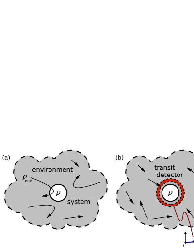
Figure 4.1: (a) In the monitoring approach the system is taken to interact at most with one environmental (quasi-)particle at a time, so that three-body collisions are excluded. Moreover, in agreement with the Markov assumption, it is assumed that the environmental particles disperse their correlation with the system before scattering again. (b) In order to consistently incorporate the state-dependence of the collision rate into the dynamic description of the scattering process, we imagine that the system is monitored continuously by a transit detector, which tells at a temporal resolution $\Delta t$ whether a particle is going to scatter off the system, or not.

The rate of collisions is then described by a positive operator $\mathsf{\Gamma}$ acting in the system-probe Hilbert space. Given the uncorrelated state $\varrho_{\operatorname{tot}}=\rho\otimes\rho_{E}$, it determines the probability of a collision to occur in a small time interval $\Delta t$,

$$\operatorname{Prob}\left(\text{C}_{\Delta t}|\rho\otimes\rho_{E}\right) = \Delta t\operatorname{tr}\left(\mathsf{\Gamma}\left[\rho\otimes\rho_{E}\right]\right)\;.$$ (4.149)

Here, $\rho_{E}$ is the stationary reduced single particle state of the environment. The microscopic definition of $\mathsf{\Gamma}$ will in general involve the current density operator of the relative motion and a total scattering cross section, see below.

The important point to note is that the information that a collision will take place changes our knowledge about the state, as described by the generalized measurement transformation (4.16). At the same time, we have to keep in mind that the measurement is not real, but is introduced here only for enabling us to account for the state dependence of the collision probability. It is therefore reasonable to take the detection process as efficient, see Sect. 4.1.3, and minimally-invasive, i.e. $\mathsf{U}_{\alpha}=\mathbbm{I}$ in (4.20), so that neither unnecessary uncertainty nor a reversible back-action is introduced. This implies that after a (hypothetical) detector click, but prior to scattering, the system-probe state will have the form

$$\mathcal{M}\left(\varrho_{\operatorname{tot}}|\text{C}_{\Delta t}\right) = \frac{\mathsf{\Gamma}^{1/2}\varrho_{\operatorname{tot}}\mathsf{\Gamma}^{1/2}}{\operatorname{tr}\left(\mathsf{\Gamma}\varrho_{\operatorname{tot}}\right)}\;.$$ (4.150)

This measurement transformation reflects our improved knowledge about the incoming two-particle wave packet, and it may be viewed as enhancing those parts which are heading towards a collision. Similarly, the absence of a detection event during $\Delta t$ changes the state, and this occurs with the probability $\operatorname{Prob}\left(\overline{\text{C}}_{\Delta t}\right)=1-\operatorname{Prob}\left(\text{C}_{\Delta t}\right)$.

Using the state transformation (4.150) we can now formulate the unconditioned system-probe state after a coarse grained time $\Delta t$ as the mixture of the colliding state transformed by the S-matrix and the untransformed non-colliding one, weighted with their respective probabilities,

$$\varrho^{\prime}_{\operatorname{tot}}\!\left(\Delta t\right) = \operatorname{Prob}\left(\text{C}_{\Delta t}|\varrho_{\operatorname{tot}}\right)\mathsf{S}\mathcal{M}\left(\varrho_{\operatorname{tot}}|\text{C}_{\Delta t}\right)\mathsf{S}^{{\dagger}}\!+\operatorname{Prob}\left(\overline{\text{C}}_{\Delta t}|\varrho_{\operatorname{tot}}\right)\mathcal{M}\left(\varrho_{\operatorname{tot}}|\overline{\text{C}}_{\Delta t}\right)$$ (4.151)

$$= \mathsf{S}\mathsf{\Gamma}^{1/2}\varrho_{\operatorname{tot}}\mathsf{\Gamma}^{1/2}\mathsf{S}^{{\dagger}}\Delta t+\varrho_{\operatorname{tot}}-\mathsf{\Gamma}^{1/2}\varrho_{\operatorname{tot}}\mathsf{\Gamma}^{1/2}\Delta t\;.$$

Here, the complementary map $\mathcal{M}\left(\cdot|\overline{\text{C}}_{\Delta t}\right)$ is fixed by the requirement that the state $\varrho_{\operatorname{tot}}$ should remain unchanged both if the collision probability vanishes, $\mathsf{\Gamma}=0$, and if the scattering has no effect, $\mathsf{S}=\mathbbm{I}$.

Focusing on the nontrivial part $\mathsf{T}$ of the two-particle S-matrix $\mathsf{S}=\mathbbm{I}+{\rm i}\mathsf{T}$ one finds that the unitarity of $\mathsf{S}$ implies that

$$\mathrm{Im}(\mathsf{T})\equiv\frac{1}{2{\rm i}}\left(\mathsf{T}-\mathsf{T}^{{\dagger}}\right) = \frac{1}{2}\mathsf{T}^{{\dagger}}\mathsf{T}\;.$$ (4.152)

Using this relation we can write the differential quotient as

$$\frac{\varrho_{\operatorname{tot}}^{\prime}\left(\Delta t\right)-\varrho_{\operatorname{tot}}}{\Delta t} = \mathsf{T}\mathsf{\Gamma}^{1/2}\varrho_{\operatorname{tot}}\mathsf{\Gamma}^{1/2}\mathsf{T}^{{\dagger}}-\frac{1}{2}\mathsf{T}^{{\dagger}}\mathsf{T}\mathsf{\Gamma}^{1/2}\varrho_{\operatorname{tot}}\mathsf{\Gamma}^{1/2}$$

$$-\frac{1}{2}\mathsf{\Gamma}^{1/2}\varrho_{\operatorname{tot}}\mathsf{\Gamma}^{1/2}\mathsf{T}^{{\dagger}}\mathsf{T}+\frac{{\rm i}}{2}\left[\mathsf{T}+\mathsf{T}^{{\dagger}},\mathsf{\Gamma}^{1/2}\varrho_{\operatorname{tot}}\mathsf{\Gamma}^{1/2}\right]\;.$$

It is now easy to arrive at a closed differential equation. We trace out the environment, assuming, in accordance with the Markov approximation, that the factorization $\varrho_{\operatorname{tot}}=\rho\otimes\rho_{E}$ is valid prior to each monitoring interval $\Delta t$. Taking the limit of continuous monitoring $\Delta t\rightarrow 0$, approximating $\operatorname{Tr}_{E}\left(\left[\operatorname{Re}(\mathsf{T}),\mathsf{\Gamma}^{1/2}\varrho_{\operatorname{tot}}\mathsf{\Gamma}^{1/2}\right]\right)\simeq\operatorname{Tr}_{E}\left(\left[\mathsf{\Gamma}^{1/2}\operatorname{Re}(\mathsf{T})\mathsf{\Gamma}^{1/2},\varrho_{\operatorname{tot}}\right]\right)$, and adding the generator $\mathsf{H}$ of the free system evolution we arrive at Hornberger2007b

$$\frac{\mathrm{d}}{\mathrm{d}t}\rho = \frac{1}{{\rm i}\hbar}\left[\mathsf{H},\rho\right]+{\rm i}\operatorname{Tr}_{E}\left(\left[\mathsf{\Gamma}^{1/2}\operatorname{Re}(\mathsf{T})\mathsf{\Gamma}^{1/2},\rho\otimes\rho_{E}\right]\right)$$ (4.154)

$$+\operatorname{Tr}_{E}\left(\mathsf{T}\mathsf{\Gamma}^{1/2}\left[\rho\otimes\rho_{E}\right]\mathsf{\Gamma}^{1/2}\mathsf{T}^{{\dagger}}\right)$$

$$-\frac{1}{2}\operatorname{Tr}_{E}\left(\mathsf{\Gamma}^{1/2}\mathsf{T}^{{\dagger}}\mathsf{T}\mathsf{\Gamma}^{1/2}\left[\rho\otimes\rho_{E}\right]\right)$$

$$-\frac{1}{2}\operatorname{Tr}_{E}\left(\left[\rho\otimes\rho_{E}\right]\mathsf{\Gamma}^{1/2}\mathsf{T}^{{\dagger}}\mathsf{T}\mathsf{\Gamma}^{1/2}\right)\;.$$

This general monitoring master equation, entirely specified by the rate operator $\mathsf{\Gamma}$, the scattering operator $\mathsf{S}=\mathbbm{I}+{\rm i}\mathsf{T}$, and the environmental state $\rho_{E}$, is non-perturbative in the sense that the collisional interaction is nowhere assumed to be weak. It is manifestly markovian even before the environmental trace is carried out, and one finds, by doing the trace in the eigenbasis of $\rho_{E}$, that is has the general Lindblad structure (8) of the generator of a quantum dynamical semigroup. The second term in (4.154), which involves a commutator, accounts for the renormalization of the system energies due to the coupling to the environment, just like (4.148), while the last three lines describe the incoherent effect of the coupling to the environment.

So far, the discussion was very general. To obtain concrete master equations one has to specify system and environment, along with the operators $\mathsf{\Gamma}$ and $\mathsf{S}$ describing their interaction. In the following applications, we will assume the environment to be an ideal Maxwell gas, whose single particle state

$$\rho_{\operatorname{gas}} = \frac{\Lambda_{\operatorname{th}}^{3}}{\Omega}\exp\left(-\beta\frac{\mathsf{p}^{2}}{2m}\right)$$ (4.155)

is characterized by the inverse temperature $\beta$, the normalization volume $\Omega$, and the thermal de Broglie wave length $\Lambda_{\operatorname{th}}$ defined in (4.128).

4.4.3 Collisional Decoherence of a Brownian Particle

As a first application of the monitoring approach, let us consider the “localization” of a mesoscopic particle by a gaseous environment. Specifically, we will assume that the mass $M$ of this Brownian particle is much greater than the mass $m$ of the gas particles. In the limit $m/M\to 0$ the energy exchange during an elastic collision vanishes, so that the mesoscopic particle will not thermalize in our description, but we expect that the off-diagonal elements of its position representation will get reduced, as discussed in Sect. 4.3.4.

This can be seen by considering the effect of the S-matrix in the limit $m/M\rightarrow 0$. In general, a collision keeps the center-of-mass invariant, and only the relative coordinates are affected. Writing $\mathsf{S}_{0}$ for the S-matrix in the center of mass frame and denoting the momentum eigenstates of the Brownian and the gas particle by $|\vec{P}\rangle$ and $|\vec{p}\rangle$, respectively, we have Taylor1972a

$$\mathsf{S}|\vec{P}\rangle|\vec{p}\rangle=\int\mathrm{d}^{3}\vec{Q}|\vec{P}-\vec{Q}\rangle|\vec{p}+\vec{Q}\rangle\langle\frac{m_{\ast}}{m}\vec{p}-\frac{m_{\ast}}{M}\vec{P}+\vec{Q}|\mathsf{S}_{0}|\frac{m_{\ast}}{m}\vec{p}-\frac{m_{\ast}}{M}\vec{P}\rangle\;,$$ (4.156)

where $m_{\ast}=Mm/\left(M+m\right)$ is the reduced mass and $\vec{Q}$ is the transfered momentum (and thus the change of the relative momentum). In the limit of a large Brownian mass we have $m_{\ast}/m\rightarrow 1$ and $m_{\ast}/M\rightarrow 0$, so that

$$\mathsf{S}|\vec{P}\rangle|\vec{p}\rangle\rightarrow\int\mathrm{d}^{3}\vec{Q}|\vec{P}-\vec{Q}\rangle|\vec{p}+\vec{Q}\rangle\langle\vec{p}+\vec{Q}|\mathsf{S}_{0}|\vec{p}\rangle\hskip 20.00003pt\text{[for $M\gg m$]}\;.$$ (4.157)

It follows that a position eigenstate $|\vec{X}\rangle$ of the Brownian particle remains unaffected by a collision,

$$\mathsf{S}|\vec{X}\rangle|\psi_{\operatorname{in}}\rangle_{\text{E}}=|\vec{X}\rangle\underbrace{\left(\mathrm{e}^{-{\rm i}\mathsf{p}\cdot\vec{X}/\hbar}\mathsf{S}_{0}\mathrm{e}^{{\rm i}\mathsf{p}\cdot\vec{X}/\hbar}\right)|\psi_{\operatorname{in}}\rangle_{\text{E}}}_{|\psi^{\left(\vec{X}\right)}_{\operatorname{out}}\rangle_{\text{E}}}\;,$$ (4.158)

as can be seen by inserting identities in terms of the momentum eigenstates. Here, $|\psi_{{\rm i}n}\rangle_{E}$ denotes an arbitrary single-particle wave packet state of a gas atom. The exponentials in (4.158) effect a translation of $\mathsf{S}_{0}$ from the origin to the position $\vec{X}$, so that the scattered state of the gas particle $|\psi^{\left(\vec{X}\right)}_{\operatorname{out}}\rangle_{\text{E}}$ depends on the location of the Brownian particle.

Just like in Sect. 4.1.1, a single collision will thus reduce the spatial coherences $\rho\left(\vec{X},\vec{X}^{\prime}\right)=\langle\vec{X}|\rho|\vec{X}^{\prime}\rangle$ by the overlap of the gas states scattered at positions $\vec{X}$ and $\vec{X}^{\prime}$,

$$\rho^{\prime}\left(\vec{X},\vec{X}^{\prime}\right) = \rho\left(\vec{X},\vec{X}^{\prime}\right)\langle\psi^{(\vec{X}^{\prime})}_{\operatorname{out}}|\psi^{\left(\vec{X}\right)}_{\operatorname{out}}\rangle_{\text{E}}\;.$$ (4.159)

The reduction factor will be the smaller in magnitude the better the scattered state of the gas particle can “resolve” between the positions $\vec{X}$ and $\vec{X}^{\prime}$.

In order to obtain the dynamic equation we need to specify the rate operator. Classically, the collision rate is determined by the product of the current density $j=n_{\operatorname{gas}}v_{\operatorname{rel}}$ and the total cross section $\sigma\left(p_{\operatorname{rel}}\right)$, and therefore $\mathsf{\Gamma}$ should be expressed in terms of the corresponding operators. This is particularly simple in the large mass limit $M\rightarrow\infty$, where $v_{\operatorname{rel}}=\left|\vec{p}/m-\vec{P}/M\right|\rightarrow\left|\vec{p}\right|/m$, so that the current density and the cross section depend only on the momentum of the gas particle, leading to

$$\mathsf{\Gamma} = \,n_{\operatorname{gas}}\frac{\left|\mathsf{p}\right|}{m}\sigma\left(\mathsf{p}\right)\;.$$ (4.160)

If the gas particle moves in a normalized wave packet heading towards the origin then the expectation value of this operator will indeed determine the collision probability. However, this expression depends only on the modulus of the velocity so that it will yield a finite collision probability even if the particle is heading away form the origin. Hence, for (4.154) to make sense either the S-matrix should be modified to keep such a non-colliding state unaffected, or $\mathsf{\Gamma}$ should contain in addition a projection to the subset of incoming states, see the discussion below.

In momentum representation, $\rho\left(\vec{P},\vec{P}^{\prime}\right)=\langle\vec{P}|\rho|\vec{P}^{\prime}\rangle$, equation (4.154) assumes the general structure

$$\partial_{t}\rho\left(\vec{P},\vec{P}^{\prime}\right) = \frac{1}{{\rm i}\hbar}\frac{P^{2}-\left(P^{\prime}\right)^{2}}{2M}\rho\left(\vec{P},\vec{P}^{\prime}\right)$$ (4.161)

$$+\int\mathrm{d}\vec{P}_{0}\mathrm{d}\vec{P}_{0}^{\prime}\,\rho\left(\vec{P}_{0},\vec{P}^{\prime}_{0}\right)M\left(\vec{P},\vec{P}^{\prime};\vec{P}_{0},\vec{P}_{0}^{\prime}\right)$$

$$-\frac{1}{2}\int\mathrm{d}\vec{P}_{0}\rho\left(\vec{P}_{0},\vec{P}^{\prime}\right)\int\mathrm{d}\vec{P}_{f}\,M\left(\vec{P}_{f},\vec{P}_{f};\vec{P}_{0},\vec{P}\right)$$

$$-\frac{1}{2}\int\mathrm{d}\vec{P}_{0}^{\prime}\rho\left(\vec{P},\vec{P}_{0}^{\prime}\right)\int\mathrm{d}\vec{P}_{f}\,M\left(\vec{P}_{f},\vec{P}_{f};\vec{P}^{\prime},\vec{P}_{0}^{\prime}\right)\;.$$

The dynamics is therefore characterized by a single complex function

$$M\left(\vec{P},\vec{P}^{\prime};\vec{P}_{0},\vec{P}_{0}^{\prime}\right) = \langle\vec{P}|\operatorname{tr}_{\operatorname{gas}}\left(\mathsf{T}\mathsf{\Gamma}^{1/2}\left[|\vec{P}_{0}\rangle\langle\vec{P}^{\prime}_{0}|\otimes\rho_{\operatorname{gas}}\right]\mathsf{\Gamma}^{1/2}\mathsf{T^{{\dagger}}}\right)|\vec{P}^{\prime}\rangle\;,$$

which has to be evaluated. Inserting the diagonal representation of the gas state (4.155)

$$\rho_{\operatorname{gas}} = \frac{(2\pi\hbar)^{3}}{\Omega}\int\mathrm{d}\vec{p}_{0}\mu\left(\vec{p}_{0}\right)\,|\vec{p}_{0}\rangle\langle\vec{p}_{0}|$$ (4.163)

it reads, with the choices (4.157) and (4.160) for $\mathsf{S}$ and $\mathsf{\Gamma}$,

$$M\!\left(\vec{P},\vec{P}^{\prime};\!\vec{P}\!-\!\vec{Q},\vec{P}^{\prime}\!-\!\vec{Q}^{\prime}\right)\! = \!\int\!\mathrm{d}\vec{p}_{1}\mathrm{d}\vec{p}_{0}\mu\left(\vec{p}_{0}\right)\delta\left(\vec{Q}+\vec{p}_{1}-\vec{p}_{0}\right)\delta\left(\vec{Q}^{\prime}+\vec{p}_{0}-\vec{p}_{1}\right)$$ (4.164)

$$\!\times\frac{n_{\operatorname{gas}}}{m}\left|\vec{p}_{0}\right|\sigma\left(\vec{p}_{0}\right)\frac{\left(2\pi\hbar\right)^{3}}{\Omega}|\langle\vec{p}_{1}|\mathsf{T}_{0}|\vec{p}_{0}\rangle|^{2}$$

$$= \delta\left(\vec{Q}-\vec{Q}^{\prime}\right)\int\mathrm{d}\vec{p}_{0}\,\mu\left(\vec{p}_{0}\right)\frac{n_{\operatorname{gas}}}{m}\left|\vec{p}_{0}\right|\sigma\left(\vec{p}_{0}\right)$$

$$\times\frac{\left(2\pi\hbar\right)^{3}}{\Omega}|\langle\vec{p}_{0}-\vec{Q}|\mathsf{T}_{0}|\vec{p}_{0}\rangle|^{2}$$

$$=: \delta\left(\vec{Q}-\vec{Q}^{\prime}\right)M_{\operatorname{in}}\left(\vec{Q}\right)\;.$$

This shows that, apart form the unitary motion, the dynamics is simply characterized by momentum exchanges described in terms of gain and loss terms,

$$\partial_{t}\rho\left(\vec{P},\vec{P}^{\prime}\right)\text{} \text{}= \frac{1}{{\rm i}\hbar}\frac{P^{2}-\left(P^{\prime}\right)^{2}}{2M}\rho\left(\vec{P},\vec{P}^{\prime}\right)+\int\mathrm{d}\vec{Q}\,\rho\left(\vec{P}-\vec{Q},\vec{P}^{\prime}-\vec{Q}\right)M_{\operatorname{in}}\left(\vec{Q}\right)$$ (4.165)

$$-\rho\left(\vec{P},\vec{P}^{\prime}\right)\int\mathrm{d}\vec{Q}M_{\operatorname{in}}\left(\vec{Q}\right)\;.$$

We still have to evaluate the function $M_{\operatorname{in}}\left(\vec{Q}\right)$, which can be clearly interpreted as the rate of collisions leading to a momentum gain $\vec{Q}$ of the Brownian particle,

$$M_{\operatorname{in}}\left(\vec{Q}\right) = \frac{n_{\operatorname{gas}}}{m}\int\mathrm{d}\vec{p}_{0}\mu\left(\vec{p}_{0}\right)\left|\vec{p}_{0}\right|\sigma\left(\vec{p}_{0}\right)\frac{\left(2\pi\hbar\right)^{3}}{\Omega}|\langle\vec{p}_{0}-\vec{Q}|\mathsf{T}_{0}|\vec{p}_{0}\rangle|^{2}\;.$$

It involves the momentum matrix element of the on-shell $\mathsf{T}_{0}$-matrix, $\mathsf{S}_{0}=1+i\mathsf{T}_{0}$, which, according to elastic scattering theory Taylor1972a , is proportional to the scattering amplitude $f$,

$$\langle\vec{p}_{f}|\mathsf{T}_{0}|\vec{p}_{i}\rangle = \frac{f(\vec{p}_{f},\vec{p}_{i})}{2\pi\hbar}\delta\left(\frac{p_{f}^{2}}{2}-\frac{p_{i}^{2}}{2}\right)\;.$$ (4.167)

The delta function ensures the conservation of energy during the collision. At first sight, this leads to an ill-defined expression since the matrix element (4.167) appears as a squared modulus in (LABEL:KHeq:Min1), so that the tree-dimensional integration is over a squared delta function.

The appearance of this problem can be traced back to our disregard of the projection to the subset of incoming states in the definition (4.160) of $\mathsf{\Gamma}$. When evaluating $M_{\operatorname{in}}$ we used the diagonal representation (4.163) for $\rho_{\operatorname{gas}}$ in terms of (improper) momentum eigenstates, which comprise both incoming and outgoing characteristics if viewed as the limiting form of a wave packet. One way of implementing the missing projection to incoming states would be to use a different convex decomposition of $\rho_{\text{gas}}$, which admits a separation into incoming and outgoing contributions Hornberger2003b . This way, $M_{\operatorname{in}}$ can indeed be calculated properly, albeit in a somewhat lengthy calculation. A shorter route to the same result sticks to the diagonal representation, but modifies the definition of $\mathsf{S}$ in a formal sense so that it keeps all outgoing state invariant. The conservation of the probability current, which must still be guaranteed by any such modification, then implies a simple rule how to deal with the squared matrix element Hornberger2003b ,

$$\frac{\left(2\pi\hbar\right)^{3}}{\Omega}\left|\langle\vec{p}_{f}|\mathsf{T}_{0}|\vec{p}_{i}\rangle\right|^{2}\longrightarrow\frac{\left|f(\vec{p}_{f},\vec{p}_{i})\right|^{2}}{p_{i}\sigma(p_{i})}\delta\left(\frac{p_{f}^{2}}{2}-\frac{p_{i}^{2}}{2}\right)\;.$$ (4.168)

Here $\sigma(p)={\int\mathrm{d}\Omega^{\prime}\,\left|f(p\vec{n}^{\prime},p\vec{n})\right|}^{2}$ is the total elastic cross section. With this replacement we obtain immediately

$$M_{\operatorname{in}}\left(\vec{Q}\right) = \frac{n_{\operatorname{gas}}}{m}\!\int\!\mathrm{d}\vec{p}_{0}\,\mu\left(\vec{p}_{0}\right)\left|f(\vec{p}_{0}-\vec{Q},\vec{p}_{0})\right|^{2}\delta\left(\frac{\vec{p}^{2}_{0}}{2}-\frac{\left(\vec{p}_{0}-\vec{Q}\right)^{2}}{2}\right)\;.$$

As one would expect, the rate of momentum changing collisions is determined by a thermal average over the differential cross section $\mathrm{d}\sigma/\mathrm{d}\Omega=\left|f\right|^{2}$.

Also for finite mass ratios $m/M$ a master equation can be obtained this way, although the calculation is more complicated Hornberger2006b ; Hornberger2008a . The resulting linear quantum Boltzmann equation then describes on equal footing the decoherence and dissipation effects of a gas on the quantum motion of a particle.

The “localizing” effect of a gas on the Brownian particle can now be seen, after going into the interaction picture in order to remove the unitary part of the evolution, and by stating the master equation in position representation. From Eqs. (4.165) and (4.4.3) one obtains

$$\partial_{t}\tilde{\rho}(\vec{X},\vec{X}^{\prime}) = -F(\vec{X}-\vec{X}^{\prime})\tilde{\rho}(\vec{X},\vec{X}^{\prime})$$ (4.170)

with localization rate Hornberger2003b

$$F(\vec{x}) = \int_{0}^{\infty}\mathrm{d}v\,\nu(v)\,\,n_{\operatorname{gas}}\,v\int\frac{\mathrm{d}\Omega_{1}\mathrm{d}\Omega_{2}}{4\pi}\left(1-\mathrm{e}^{{\rm i}mv\left(\vec{n}_{1}-\vec{n}_{2}\right)\cdot\vec{x}/\hbar}\right)$$ (4.171)

$$\times{\left|f(mv\vec{n}_{2},mv\vec{n}_{1})\right|}^{2}\;.$$

Here, the unit vectors $\vec{n}_{1},\vec{n}_{2}$ are the directions of incoming and outgoing gas particles associated to the elements of solid angle $\mathrm{d}\Omega_{1}$ and $\mathrm{d}\Omega_{2}$ and $\nu\left(v\right)$ is the velocity distribution in the gas. Clearly, $F\left(\vec{x}\right)$ determines how fast the spatial coherences corresponding to the distance $\vec{x}$ decay.

One angular integral in (4.171) can be performed in the case of isotropic scattering, $f(\vec{p}_{f},\vec{p}_{i})=f\left(\cos\left(\vec{p}_{f},\vec{p}_{i}\right);E=p_{i}^{2}/2m\right)$. In this case,

$$F(\vec{x}) = \int_{0}^{\infty}\,\mathrm{d}v\,\nu(v)\,\,n\,_{\operatorname{gas}}v\left\{\sigma(mv)-2\pi\int_{-1}^{1}\mathrm{d}\left(\cos\theta\right)\left|f\left(\cos\theta;E=\frac{m}{2}v^{2}\right)\right|^{2}\right.$$ (4.172)

$$\left.\phantom{\int_{0}^{\infty}\,\mathrm{d}v\,\nu(v)\,\,n\,_{\operatorname{gas}}v\left\{\sigma_{\operatorname{tot}}(v)-\right.}\times\,\operatorname{sinc}\left(2\sin\left(\frac{\theta}{2}\right)\frac{mv\left|\vec{x}\right|}{\hbar}\right)\right\}\;,$$

with $\operatorname{sinc}(x)=\sin(x)/x$ and $\theta$ the (polar) scattering angle.

Figure 4.2: The localization rate (4.172) describing the loss of wave-like behavior in a Brownian particle state saturates for large distances at the average collision rate. In contrast, the Caldeira–Leggett model predicts a quadratic increase beyond all bounds (dashed line), see (4.126). This indicates that linear coupling models should be taken with care if time scales are involved that differ strongly from the dissipation time scale.

The argument of the sinc function is equal to the momentum exchange during the collision times the distance in units of $\hbar$. As $\left|\vec{X}-\vec{X}^{\prime}\right|\longrightarrow 0$ the sinc approaches unity and the angular integral yields the total cross section $\sigma$ so that the localization rate vanishes, as required. At very small distances, a second order expansion in the distance $\vec{x}$ is permissible and one obtains a quadratic dependence Joos1985a , such as predicted by the Caldeira–Leggett model, see Eq. (4.127). However, once the distance $\left|\vec{X}-\vec{X}^{\prime}\right|$ is sufficiently large so that the scattered state can resolve whether the collision took place at position $\vec{X}$ or $\vec{X}^{\prime}$ the sinc function in (4.172) suppresses the integrand. It follows that in the limit of large distances the localization rate saturates, at a value given by the average collision rate $F(\infty)=\left\langle\sigma vn_{\operatorname{gas}}\right\rangle$, see Figure 4.2.

Decoherence in this saturated regime of large separations has been observed, in good agreement with this theory, in molecular interference experiments in the presence of various gases Hornberger2003a . The intermediate regime between quadratic increase and saturation was also seen in such experiments on momentum-exchange mediated decoherence, by studying the influence of the heat radiation emitted by fullerene molecules on the visibility of their interference pattern Hackermuller2004a .

As a conclusion of this section, we see that the scattering approach permits to incorporate realistic microscopic interactions transparently and without approximation in the interaction strength. The results show clearly that linear coupling models, which imply that decoherence rates grow above all bounds, have a limited range of validity. They cannot be judged by their success in describing dissipative phenomena. Frequent claims of “universality” in decoherence behavior, which are based on these linear coupling models, are therefore to be treated with care.

4.4.4 Decoherence of a Quantum Dot

As a second application of the monitoring approach, let us see how the dynamics of an immobile object with discrete internal structure, such as an implementation of a quantum dot, gets affected by an environment of ideal gas particles. For simplicity, we take the gas again in the Maxwell state (4.155), though different dispersion relations, e.g. in the case of phonon quasi-particles, could be easily incorporated. The interaction between system and gas will be described in terms of the in general inelastic scattering amplitudes determined by the interaction potential.

In the language of scattering theory the energy eigenstates of the non-motional degrees of freedom are called channels. In our case of a structureless gas they form a discrete basis of the system Hilbert space. In the following, the notation $|\alpha\rangle$, not to be confused with the coherent states of Sect. 4.3.4, will be used to indicate the system eigenstates of energy $E_{\alpha}$. In this channel basis, $\rho_{\alpha\beta}=\langle\alpha|\rho|\beta\rangle$, the equation of motion (4.154) takes on the form of a general discrete master equation of Lindblad type,

$$\partial_{t}\rho_{\alpha\beta} = \frac{E_{\alpha}+\varepsilon_{\alpha}-E_{\beta}-\varepsilon_{\beta}}{{\rm i}\hbar}\rho_{\alpha\beta}+\sum_{\alpha_{0}\beta_{0}}\rho_{\alpha_{0}\beta_{0}}\,M_{\alpha\beta}^{\alpha_{0}\beta_{0}}$$ (4.173)

$$-\frac{1}{2}\sum_{\alpha_{0}}\rho_{\alpha_{0}\beta}\,\,\sum_{\gamma}M_{\gamma\gamma}^{\alpha_{0}\alpha}-\frac{1}{2}\sum_{\beta_{0}}\rho_{\alpha\beta_{0}}\,\sum_{\gamma}M_{\gamma\gamma}^{\beta\beta_{0}}\;.$$

The real energy shifts $\varepsilon_{\alpha}$ given below describe the coherent modification of the system energies due to the presence of the environment. They are due to the second term in  (4.154) and are the analogue of the Lamb shift (4.148) encountered in the weak coupling calculation. The incoherent effect of the environment, on the other hand, is described by the set of complex rate coefficients

$$M_{\alpha\beta}^{\alpha_{0}\beta_{0}} = \langle\alpha|\operatorname{Tr}_{E}\left(\mathsf{T}\mathsf{\Gamma}^{1/2}\left[|\alpha_{0}\rangle\langle\beta_{0}|\otimes\rho_{\operatorname{gas}}\right]\mathsf{\Gamma}^{1/2}\mathsf{T}^{{\dagger}}\right)|\beta\rangle\;.$$ (4.174)

In order to calculate these quantities we need again to specify the rate operator $\mathsf{\Gamma}$. In the present case, it is naturally given in terms of the current density operator $\mathsf{j}=n_{\operatorname{gas}}\mathsf{p}/m$ of the impinging gas particles multiplied by the channel-specific total scattering cross sections $\sigma\left(\vec{p},\alpha\right)$,

$$\mathsf{\Gamma} = \sum_{\alpha}|\alpha\rangle\langle\alpha|\otimes n_{\operatorname{gas}}\frac{\left|\mathsf{p}\right|}{m}\sigma\left(\mathsf{p},\alpha\right)\;.$$ (4.175)

Like in Sect. 4.4.3, this operator should in principle contain a projection to the subset of incoming states of the gas particle. Again, this can be accounted for in two different ways in the calculation of the rates (4.174). By using a non-diagonal decomposition of $\rho_{\operatorname{gas}}$, which permits to disregard the outgoing states, one obtains

$$M_{\alpha\beta}^{\alpha_{0}\beta_{0}} = \chi_{\alpha\beta}^{\alpha_{0}\beta_{0}}\frac{n_{\operatorname{gas}}}{m^{2}}\int\mathrm{d}\vec{p}\,\,\mathrm{d}\vec{p}_{0}\mu\left(\vec{p}_{0}\right)f_{\alpha\alpha_{0}}\left(\vec{p},\vec{p}_{0}\right)$$ (4.176)

$$\times f_{\beta\beta_{0}}^{\ast}\left(\vec{p},\vec{p}_{0}\right)\delta\left(\frac{\vec{p}^{2}-\vec{p}_{0}^{2}}{2m}+E_{\alpha}-E_{\alpha_{0}}\right)\;,$$

with the Kronecker-like factor

$$\chi_{\alpha\beta}^{\alpha_{0}\beta_{0}} := \left\{\begin{array}[]{ll}1&\text{if $E_{\alpha}-E_{\alpha_{0}}=E_{\beta}-E_{\beta_{0}}$}\\ 0&\text{otherwise}\;.\end{array}\right.$$ (4.179)

The energy shifts are determined the real parts of the forward scattering amplitude,

$$\varepsilon_{\alpha} = -2\pi\hbar^{2}\frac{n_{\operatorname{gas}}}{m}\int\mathrm{d}\vec{p}_{0}\mu\left(\vec{p}_{0}\right)\operatorname{Re}\left[f_{\alpha\alpha}\left(\vec{p}_{0},\vec{p}_{0}\right)\right].$$ (4.180)

Some details of this calculation can be found in Hornberger2007b . Rather than repeating them here we note that the result (4.176) can be obtained directly by using the diagonal representation (4.163) of $\rho_{\operatorname{gas}}$ and the multichannel-generalization of the replacement rule (4.168),

$$\frac{\left(2\pi\hbar\right)^{3}}{\Omega}\langle\alpha\vec{p}|\mathsf{T}|\alpha_{0}\vec{p}_{0}\rangle\langle\beta_{0}\vec{p}_{0}|\mathsf{T}^{{\dagger}}|\beta\vec{p}\rangle \rightarrow \frac{\chi_{\alpha\beta}^{\alpha_{0}\beta_{0}}}{p_{0}m}\frac{f_{\alpha\alpha_{0}}\left(\vec{p},\vec{p}_{0}\right)f^{\ast}_{\beta\beta_{0}}\left(\vec{p},\vec{p}_{0}\right)}{\sqrt{\sigma\left(p_{0},\alpha_{0}\right)\sigma\left(p_{0},\beta_{0}\right)}}\;\;\;\;$$ (4.181)

$$\times\delta\left(\frac{\vec{p}^{2}-\vec{p}_{0}^{2}}{2m}+E_{\alpha}-E_{\alpha_{0}}\right)\;.$$

The expression for the complex rates simplifies further if the scattering amplitudes are rotationally invariant, $f_{\alpha\alpha_{0}}\left(\cos\left(\vec{p},\vec{p}_{0}\right);E=p_{0}^{2}/2m\right)$. In this case we have

$$M_{\alpha\beta}^{\alpha_{0}\beta_{0}} = \chi_{\alpha\beta}^{\alpha_{0}\beta_{0}}\int_{0}^{\infty}\mathrm{d}v\nu\left(v\right)n_{\operatorname{gas}}v_{\operatorname{out}}\left(v\right)2\pi\int_{-1}^{1}\mathrm{d}\left(\cos\theta\right)$$ (4.182)

$$\times f_{\alpha\alpha_{0}}\left(\cos\theta;E=\frac{m}{2}v^{2}\right)f_{\beta\beta_{0}}^{\ast}\left(\cos\theta;E=\frac{m}{2}v^{2}\right)$$

with $\nu\left(v\right)$the velocity distribution like in (4.172), and

$$v_{\operatorname{out}}\left(v\right) = \sqrt{v^{2}-\frac{2}{m}\left(E_{\alpha}-E_{\alpha_{0}}\right)}$$ (4.183)

the velocity of a gas particle after a possibly inelastic collision.

This shows that limiting cases of (4.173) display the expected dynamics. For the populations $\rho_{\alpha\alpha}$ it reduces to a rate equation, where the cross sections $\sigma_{\alpha\alpha_{0}}\left(E\right)=2\pi\int\mathrm{d}\left(\cos\theta\right)\left|f_{\alpha\alpha_{0}}\left(\cos\theta;E\right)\right|^{2}$ for scattering from channel $\alpha_{0}$ to $\alpha$ determine the transition rates,

$$M_{\alpha\alpha}^{\alpha_{0}\alpha_{0}} = \int\mathrm{d}v\nu\left(v\right)n_{\operatorname{gas}}v_{\operatorname{out}}\left(v\right)\sigma_{\alpha\alpha_{0}}\left(\frac{m}{2}v^{2}\right)\;.$$ (4.184)

In the case of purely elastic scattering, on the other hand, i.e. for $M_{\alpha\beta}^{\alpha_{0}\beta_{0}}=M_{\alpha\beta}^{\alpha\beta}\delta_{\alpha\alpha_{0}}\delta_{\beta\beta_{0}}$, the coherences are found to decay exponentially,

$$\partial_{t}\left|\rho_{\alpha\beta}\right| = -\gamma_{\alpha\beta}^{\operatorname{elastic}}\left|\rho_{\alpha\beta}\right|\;.$$ (4.185)

The corresponding pure dephasing rates are determined by the difference of the scattering amplitudes,

$$\gamma_{\alpha\beta}^{\operatorname{elastic}} = \pi\int\mathrm{d}v\nu\left(v\right)n_{\operatorname{gas}}v_{\operatorname{out}}\left(v\right)\int_{-1}^{1}\mathrm{d}\left(\cos\theta\right)$$ (4.186)

$$\times\left|f_{\alpha\alpha}\left(\cos\theta;\frac{m}{2}v^{2}\right)-f_{\beta\beta}\left(\cos\theta;\frac{m}{2}v^{2}\right)\right|^{2}\;.$$

As one expects in this case, the better the scattering environment can distinguish between system states $|\alpha\rangle$ and $|\beta\rangle$ the more coherence is lost in this elastic process.

In the general case, the decay of off-diagonal elements will be due to a combination of elastic and inelastic processes. Although little can be said without specifying the interaction, it is clear that the integral over $\left|f_{\alpha\alpha}-f_{\beta\beta}\right|^{2}$ in (4.186), a “decoherence cross section” without classical interpretation, is not related to the inelastic cross sections characterizing the population transfer, and may be much larger. In this case, the resulting decoherence will be again much faster than the corresponding relaxation time scales.

4.5 Robust States and the Pointer Basis

We have seen that, even though the decoherence predictions of linear coupling models has to be taken with great care, the general observation remains valid that the loss of coherence may occur on a time scale $\gamma_{\operatorname{deco}}^{-1}$ that is much shorter the relaxation time $\gamma^{-1}$. Let us therefore return to the general description of open systems in terms of a semigroup generator $\mathcal{L}$, and ask what we can say about a general state after a time $t$ which is still small compared to the relaxation time, but much larger than the decoherence time scale. From a classical point of view, which knows only about relaxation, the state has barely changed, but in the quantum description it may now be well approximated by a mixture determined by particular projectors $\mathsf{P}_{\ell}$,

$$\mathrm{e}^{\mathcal{L}t}:\rho\xrightarrow{\gamma_{\operatorname{deco}}^{-1}\ll t\ll\gamma^{-1}}\rho_{t}\simeq\rho^{\prime}=\sum_{\ell}\operatorname{tr}(\rho\mathsf{P}_{\ell})\,\mathsf{P}_{\ell}.$$ (4.187)

This set of projectors {$\mathsf{P}_{\ell}$}, which depend at most weakly on $t$, is called pointer basis Zurek1981a or set of robust states Diosi2000a . It is distinguished by the fact that a system prepared in such a state is hardly affected by the environment, while a superposition of two distinct pointer states decoheres so rapidly that it is never observed in practice.

We encountered this behavior with the damped harmonic oscillator discussed in Sect. 4.3.4. There the coherent oscillator states remained pure under Markovian dynamics, while superpositions between (macroscopically distinct) coherent states decayed rapidly. Hence, in this case the coherent states $\mathsf{P}_{\alpha}=|\alpha\rangle\langle\alpha|$ can be said to form an (over-complete) set of robust states, leading to the mixture

$$\rho^{\prime}=\int\mathrm{d}\mu\left(\alpha\right)\operatorname{tr}(\rho\mathsf{P}_{\alpha})\mathsf{P}_{\alpha}\;,$$ (4.188)

with appropriate measure $\mu$.

The name pointer basis is well-fitting because the existence of such robust states is a prerequisite for the description of an ideal measurement device in a quantum framework. A macroscopic—and therefore decohering—apparatus implementing the measurement of an observable $\mathsf{A}$ is ideally constructed in such a way that macroscopically distinct positions of the “pointer” are obtained for the different eigenstates of $\mathsf{A}$. Provided these pointer positions of the device are robust, the correct values are observed with certainty if the quantum system is in an eigenstate of the observable. Conversely, if the quantum system is not in an eigenstate of $\mathsf{A}$, the apparatus will not end up in a superposition of pointer positions, but be found at a definite position, albeit probabilistically, with a probability given by the Born rule.

The main question regarding pointer states is, given the environmental coupling or the generator $\mathcal{L}$, what determines whether a state is robust or not, and how can we determine the set of pointer states without solving the master equation for all initial states. It is fair to say that this issue is not fully understood, except for very simple model environments, nor is it even clear how to quantify robustness.

An obvious ansatz, due to Zurek Zurek2003a ; Zurek1993a , is to sort all pure states in the Hilbert space according to their (linear) entropy production rate, or rate of loss of purity,

$$\partial_{t}\mathsf{S}_{\operatorname{lin}}[\rho]=-2\operatorname{tr}\left(\rho\mathcal{L}(\rho)\right)\;.$$ (4.189)

It has been called “predictability sieve” since the least entropy producing and therefore most predictable states are candidate pointer states Zurek2003a .

In the following, a related approach will be described, following the presentation in Strunz2002a ; Gisin1995a . It is based on a time evolution equation for robust states. Since such an equation must distinguish particular states from their linear superpositions, it is necessarily nonlinear.

4.5.1 Nonlinear Equation for Robust States

We seek a nonlinear time evolution equation for robust pure states $\mathsf{P}_{t}$ which, on the one hand, preserves their purity, and on the other, keeps them as close as possible to the evolved state following the master equation.

A simple nonlinear equation keeping a pure state pure is given by the following extension of the Heisenberg form for the infinitesimal time step,

$$\mathsf{P}_{t+\delta t}=\mathsf{P}_{t}+\delta t\left(\frac{1}{{\rm i}}[\mathsf{A}_{t},\mathsf{P}_{t}]+[\mathsf{P}_{t},[\mathsf{P}_{t},\mathsf{B}_{t}]]\right)\;,$$ (4.190)

where $\mathsf{A}\text{}\mathsf{}$ and $\mathsf{B}$ are hermitian operators. In fact, the unitary part can be absorbed into the nonlinear part by introducing the hermitian operator $\mathsf{X}_{t}=-{\rm i}[\mathsf{A}_{t},\mathsf{P}_{t}]+\mathsf{B}_{t}$. It “generates” the infinitesimal time translation of the projectors (and may be a function of $\mathsf{P}_{t}$),

$$\left.\mathsf{P}_{t+\delta t}=\mathsf{P}_{t}+\delta t[\mathsf{P}_{t},[\mathsf{P}_{t},\mathsf{X}_{t}]\right]\;.$$ (4.191)

With this choice one confirms easily that the evolved operator has indeed the properties of a projector, to leading order in $\delta t$,

$$\mathsf{P}_{t+\delta t}^{{\dagger}}=\mathsf{P}_{t+\delta t}$$ (4.192)

and

$$\left(\mathsf{P}_{t+\delta t}\right)^{2} = \mathsf{P}_{t+\delta t}+O(\delta t^{2})\;.$$ (4.193)

The corresponding differential equation reads

$$\partial_{t}\mathsf{P}_{t}=\frac{\mathsf{P}_{t+\delta t}-\mathsf{P}_{t}}{\delta t}=\left[\mathsf{P}_{t},\left[\mathsf{P}_{t},\mathsf{X}_{t}\right]\right]\;.$$ (4.194)

To determine the operator $\mathsf{X}_{t}$ one minimizes the distance between the time derivatives of the truly evolved state and the projector. If we visualize the pure states as lying on the boundary of the convex set of mixed states, then a pure state will in general dive into the interior under the time evolution generated by $\mathcal{L}$. The minimization chooses the operator $\mathsf{X}_{t}$ in such a way that $\mathsf{P}_{t}$ sticks to the boundary, while remaining as close as possible to the truly evolved state.

The (Hilbert-Schmidt) distance between the time derivatives can be calculated as

$$\|\underbrace{\mathcal{L}(\mathsf{P}_{t})}_{\equiv\mathsf{Z}}-\partial_{t}\mathsf{P}_{t}\|^{2}_{\operatorname{HS}\mathsf{}} = \operatorname{tr}\left[\left(\mathsf{Z}-\left[\mathsf{P}_{t},\left[\mathsf{P}_{t},\mathsf{X}_{t}\right]\right]\right)^{2}\right]$$ (4.195)

$$= \operatorname{tr}\left(\mathsf{Z}^{2}-2(\mathsf{Z}^{2}\mathsf{P}_{t}-\left(\mathsf{Z}\mathsf{P}_{t}\right)^{2})\right)$$

$$+2\operatorname{tr}\left((\mathsf{Z}-\mathsf{X})^{2}\mathsf{P}_{t}-\left(\left(\mathsf{Z}-\mathsf{X}\right)\mathsf{P}_{t}\right)^{2}\right)\;.$$

We note that the first term is independent of $\mathsf{X}$, whereas the second one is non-negative. With the obvious solution $\mathsf{X}_{t}=\mathsf{Z}\equiv\mathcal{L}(\mathsf{P}_{t})$ one gets a nonlinear evolution equation for robust states $\mathsf{P}_{t}$, which is trace and purity preserving Gisin1995a ,

$$\partial_{t}\mathsf{P}_{t}=[\mathsf{P}_{t},[\mathsf{P}_{t},\mathcal{L}(\mathsf{P}_{t})]]\;.$$ (4.196)

It is useful to write down the equation in terms of the vectors $|\xi\rangle$ which correspond to the pure state $\mathsf{P}_{t}=|\xi\rangle\langle\xi|$,

$$\partial_{t}|\xi\rangle=[\mathcal{L}(|\xi\rangle\langle\xi|)-\underbrace{\langle\xi|\mathcal{L}(|\xi\rangle\langle\xi|)|\xi\rangle}_{\text{``decay rate''}}]|\xi\rangle\;.$$ (4.197)

If we take $\mathcal{L}$ to be of the Lindblad form (4.79) the equation reads

$$\partial_{t}|\xi\rangle = \frac{1}{{\rm i}\hbar}\mathsf{H}|\xi\rangle+\sum_{k}\gamma_{k}\left[\langle\mathsf{L}_{k}^{{\dagger}}\rangle_{\xi}\left(\mathsf{L}_{k}-\left\langle\mathsf{L}_{k}\right\rangle_{\xi}\right)-\frac{1}{2}\left(\mathsf{L}_{k}^{{\dagger}}\mathsf{L}-\langle\mathsf{L}_{k}^{{\dagger}}\mathsf{L}_{k}\rangle\right)\right]\,|\xi\rangle$$ (4.198)

$$-\frac{1}{{\rm i}\hbar}\langle\mathsf{H}\rangle_{\xi}|\xi\rangle\;.$$

Its last term is usually disregarded because it gives rise only to an additional phase if $\langle\mathsf{H}\rangle_{\xi}$ is constant. The meaning of the nonlinear equation (4.198) is best studied in terms of concrete examples.

4.5.2 Applications

Damped Harmonic Oscillator

Let us start with the damped harmonic oscillator discussed in Sect. 4.3.4. By setting $\mathsf{H}=\hbar\omega\mathsf{a}^{{\dagger}}\mathsf{a}$ and $\mathsf{L}=\mathsf{a}$ (4.198) turns into

$$\partial_{t}|\xi\rangle=-{\rm i}\omega\mathsf{a}^{{\dagger}}\mathsf{a}|\xi\rangle+\gamma\left(\langle\mathsf{a}^{{\dagger}}\rangle_{\xi}(\mathsf{a}-\left\langle\mathsf{a}\right\rangle_{\xi})-\frac{1}{2}\left(\mathsf{a}^{{\dagger}}\mathsf{a}-\langle\mathsf{a}^{{\dagger}}\mathsf{a}\rangle_{\xi}\right)\right)|\xi\rangle\;.$$ (4.199)

Note that the first term of the non-unitary part vanishes if $|\xi\rangle$ is a coherent state, i.e. an eigenstate of $\mathsf{a}$. This suggests the ansatz $|\xi\rangle=|\alpha\rangle$ which leads to

$$\partial_{t}|\alpha\rangle=\left[\left(-{\rm i}\omega-\frac{\gamma}{2}\right)\alpha\mathsf{a}^{{\dagger}}+\frac{\gamma}{2}|\alpha|^{2}\right]|\alpha\rangle\;.$$ (4.200)

It is easy to convince oneself that this equation is solved by

$$|\alpha_{t}\rangle=|\alpha_{0}\mathrm{e}^{-{\rm i}\omega t-\gamma t/2}\rangle=\mathrm{e}^{-|\alpha_{t}|^{2}/2}\mathrm{e}^{\alpha_{t}\mathsf{a}^{{\dagger}}}|0\rangle$$ (4.201)

with $\alpha_{t}=\alpha_{0}\exp\left(-{\rm i}\omega t-\gamma t/2\right)$. It shows that the predicted robust states are indeed given by the slowly decaying coherent states encountered in Sect. 4.3.4.

Quantum Brownian Motion

A second example is given by the Brownian motion of a quantum particle. The choice

$$\mathsf{H}=\frac{\mathsf{p}^{2}}{2m}\hskip 10.00002pt \operatorname{and} \hskip 10.00002pt\mathsf{L}=\frac{\sqrt{8\pi}}{\Lambda_{\operatorname{th}}}\mathsf{x}$$ (4.202)

yields a master equation of the form (4.117) but without the dissipation term. Inserting these operators into (4.198) leads to

$$\partial_{t}|\xi\rangle=\frac{\mathsf{p}^{2}}{2m{\rm i}\hbar}|\xi\rangle-\gamma\frac{4\pi}{\Lambda_{\operatorname{th}}^{2}}[(\mathsf{x}-\left\langle\mathsf{x}\right\rangle_{\xi})^{2}-\underbrace{\langle(\mathsf{x}-\left\langle\mathsf{x}\right\rangle_{\xi})^{2}\rangle_{\xi}}_{\sigma^{2}_{\xi}(\mathsf{x})}]|\xi\rangle\;.$$ (4.203)

The action of the non-unitary term is apparent in the position representation, $\xi(x)=\langle x|\xi\rangle$. At positions $x$ which are distant from mean position $\left\langle\mathsf{x}\right\rangle_{\xi}$ as compared to the dispersion $\sigma_{\xi}(\mathsf{x})=\big{\langle}\left(\mathsf{x}-\langle\mathsf{x}\rangle_{\xi}\right)^{2}\big{\rangle}_{\xi}^{1/2}$ the term is negative and the value $\xi(x)$ gets suppressed. Conversely, the part of the wave function close to the mean position gets enhanced,

$$\langle x|\xi\rangle=\left\{\begin{array}[]{ll}\text{suppressed}&\text{if }|x-\left\langle\mathsf{x}\right\rangle_{\xi}|>\sigma_{\xi}(\mathsf{x})\\ \text{enhanced }&\text{if }|x-\left\langle\mathsf{x}\right\rangle_{\xi}|<\sigma_{\xi}(\mathsf{x})\;.\end{array}\right.$$ (4.204)

This localizing effect is countered by the first term in (4.203) which causes the dispersive broadening of the wave function. Since both effects compete we expect stationary, soliton-like solutions of the equation.

Indeed, a Gaussian ansatz for $|\xi\rangle$ with ballistic motion, i.e. $\left\langle\mathsf{p}\right\rangle_{\xi}=p_{0}$, $\left\langle\mathsf{x}\right\rangle_{\xi}=x_{0}+p_{0}t/m$, and a fixed width $\sigma_{\xi}(\mathsf{x})=\sigma_{0}$ solves (4.203) provided Diosi2000a

$$\sigma_{0}^{2}=\frac{1}{4\pi}\sqrt{\frac{k_{B}T}{2\hbar\gamma}}\Lambda_{\operatorname{th}}^{2}=\left(\frac{\hbar^{3}}{8\gamma m^{2}k_{B}T}\right)^{1/2}\;,$$ (4.205)

see (4.128). As an example, let us consider a dust particle with a mass of 10 $\mu$g in the interstellar medium interacting only with the microwave background of $T=2.7\,\mathrm{K}$. Even if we take a very small relaxation rate of $\gamma=1/(13.7\times 10^{9}\,{\rm y})$, corresponding to the inverse age of the universe, the width of the solitonic wave packet describing the center of mass is as small as $2$ pm. This sub-atomic value demonstrates again the remarkable efficiency of the decoherence mechanism to induce classical behavior in the quantum state of macroscopic objects.

Acknowledgments

Many thanks to Álvaro Tejero Cantero who provided me with his notes, typed with the lovely TEXmacs program during the lecture. The present text is based on his valuable input. I am also grateful to Marc Busse and Bassano Vacchini for helpful comments on the manuscript.

This work was supported by the Emmy Noether program of the DFG.

Contents

toc

References

• (1) E. Joos, H. D. Zeh, C. Kiefer, D. Giulini, J. Kupsch, and I.-O. Stamatescu: Decoherence and the Appearance of a Classical World in Quantum Theory, 2nd edn. ( Springer, Berlin 2003)
• (2) H.-P. Breuer and F. Petruccione: The Theory of Open Quantum Systems (Oxford University Press, Oxford 2002)
• (3) W. T. Strunz: Decoherence in Quantum Physics. In: Coherent Evolution in Noisy Environments, Lecture Notes in Physics 611, ed. by A. Buchleitner and K. Hornberger (Springer, Berlin 2002)
• (4) G. Bacciagaluppi: The Role of Decoherence in Quantum Mechanics. In: The Stanford Encyclopedia of Philosophy, ed. by E. N. Zalta (Stanford University, 2005) http://plato.stanford.edu.
• (5) M. Schlosshauer: Decoherence, the measurement problem, and interpretations of quantum mechanics, Rev. Mod. Phys. 76, 1267–1305 (2004)
• (6) W. H. Zurek: Decoherence, Einselection, and the Quantum Origins of the Classical, Rev. Mod. Phys. 75, 715–775 (2003)
• (7) J. P. Paz and W. H. Zurek: Environment-Induced Decoherence and the Transition From Quantum to Classical. In: Les Houches Summer School Series, vol. 72, ed. by R. Kaiser, C. Westbrook, and F. David (Springer-Verlag, 2001) pp. 533
• (8) A. Bassi and G. Ghirardi: Dynamical Reduction Models, Phys. Rep. 379, 257 (2003)
• (9) K. Kraus: States, Effects and Operations: Fundamental Notions of Quantum Theory, ( Springer, Berlin 1983)
• (10) P. Busch, P. J. Lahti, and P. Mittelstaed: The Quantum Theory of Measurement (Springer-Verlag, Berlin 1991)
• (11) A. S. Holevo: Statistical Structure of Quantum Theory ( Springer, Berlin 2001)
• (12) C. W. Helstrom: Quantum Detection and Estimation Theory ( Academic Press, New York 1976)
• (13) A. Chefles: Quantum state discrimination, Contemp. Phys. 41, 401–424 (2000)
• (14) G. M. Palma, K.-A. Suominen, and A. K. Ekert: Quantum computers and dissipation, Proc. R. Soc. Lond. A 452, 567 (1996)
• (15) D. F. Walls and G. J. Milburn: Quantum Optics ( Springer, Berlin 1994)
• (16) M. Hillery, R. F. O’Connell, M. O. Scully, and E. P. Wigner: Distribution functions in physics: Fundamentals, Phys. Rep. 106, 121–167 (1984)
• (17) U. Weiss: Quantum Dissipative Systems, 2nd edn. ( World Scientific, Singapore 1999)
• (18) P. Machnikowski: Change of decoherence scenario and appearance of localization due to reservoir anharmonicity, Phys. Rev. Lett. 96, 140405 (2006)
• (19) Y. Imry: Elementary explanation of the inexistence of decoherence at zero temperature for systems with purely elastic scattering, Arxiv preprint cond-mat/0202044 (2002)
• (20) R. Doll, M. Wubs, P. Hänggi, and S. Kohler: Limitation of entanglement due to spatial qubit separation, Europhys. Lett. 76, 547–553 (2006)
• (21) E. B. Davies: Quantum Theory of Open Systems (Academic Press, London 1976)
• (22) H. Spohn: Kinetic equations from Hamiltonian dynamics: Markovian limits, Rev. Mod. Phys. 52, 569–615 (1980)
• (23) R. Alicki and K. Lendi: Quantum Dynamical Semigroups and Applications (Springer, Berlin 1987)
• (24) F. Petruccione and B. Vacchini: Quantum description of Einstein’s Brownian motion, Phys. Rev. E 71, 046134 (2005)
• (25) H. Carmichael: An Open Systems Approach to Quantum Optics (Springer, Berlin 1993)
• (26) K. Mølmer, Y. Castin, and J. Dalibard: Monte Carlo wave-function method in quantum optics, J. Opt. Soc. Am. B 10, 524–538 (1993)
• (27) M. B. Plenio and P. L. Knight: The quantum-jump approach to dissipative dynamics in quantum optics, Rev. Mod. Phys. 70, 101–144 (1998)
• (28) J. M. Raimond, M. Brune, and S. Haroche, Colloquium: Manipulating Quantum Entanglement with Atoms and Photons in a Cavity, Rev. Mod. Phys. 73, 565–582 (2001)
• (29) S. Haroche: Mesoscopic superpositions and decoherence in quantum optics. In: Quantum entanglement and information processing, Les Houches 2003, ed. by D. Estève, J.-M. Raimond, and J. Dalibard (Elsevier, Amsterdam 2004)
• (30) A. O. Caldeira and A. J. Leggett: Path Integral Approach to Quantum Brownian Motion, Physica A 121, 587–616 (1983)
• (31) W. G. Unruh and W. H. Zurek: Reduction of a Wave Packet in Quantum Brownian Motion, Phys. Rev. D 40, 1071–1094 (1989)
• (32) L. Diósi: On high temperature Markovian equation for quantum Brownian motion, Europhys. Lett. 22, 1-3 (1993)
• (33) L. Lukacs: Characteristic Functions (Griffin, London 1966)
• (34) K. Hornberger: Monitoring approach to open quantum dynamics using scattering theory, Europhys. Lett. 77, 50007 (2007).
• (35) J. R. Taylor: Scattering Theory (John Wiley & Sons, New York 1972)
• (36) K. Hornberger and J. E. Sipe: Collisional Decoherence Reexamined, Phys. Rev. A 68, 012105 (2003)
• (37) K. Hornberger: Master equation for a quantum particle in a gas, Phys. Rev. Lett. 97, 060601 (2006)
• (38) K. Hornberger and B. Vacchini: Monitoring derivation of the quantum linear Boltzmann equation, Phys. Rev. A 77, 022112 (2009)
• (39) E. Joos and H. D. Zeh: The Emergence of Classical Properties Through Interaction with the Environment, Z. Phys. B: Condens. Matter 59, 223–243 (1985)
• (40) K. Hornberger, S. Uttenthaler, B. Brezger, L. Hackermüller, M. Arndt, and A. Zeilinger: Collisional Decoherence Observed in Matter Wave Interferometry, Phys. Rev. Lett. 90, 160401 (2003)
• (41) L. Hackermüller, K. Hornberger, B. Brezger, A. Zeilinger, and M. Arndt: Decoherence of Matter Waves by Thermal Emission of Radiation, Nature 427, 711–714 (2004)
• (42) R. Dümcke: The low density limit for an N-level system interacting with a free bose or fermi gas, Commun. Math. Phys. 97, 331–359 (1985)
• (43) W. H. Zurek: Pointer Basis of Quantum Apparatus: Into What Mixture Does the Wave Packet Collapse?, Phys. Rev. D 24, 1516–1525 (1981)
• (44) L. Diósi and C. Kiefer: Robustness and Diffusion of Pointer States, Phys. Rev. Lett. 85, 3552–3555 (2000)
• (45) W. H. Zurek, S. Habib, and J. P. Paz: Coherent states via decoherence, Phys. Rev. Lett. 70, 1187–1190 (1993)
• (46) N. Gisin and M. Rigo: Relevant and irrelevant nonlinear Schrödinger equations, J. Phys. A: Math. Gen. 28, 7375–7390 (1995)