Entanglement of three-qubit geometry

Abstract

Geometric quantum mechanics aims to express the physical properties of quantum systems in terms of geometrical features preferentially selected in the space of pure states. Geometric characterisations are given here for systems of one, two, and three spin-$\textstyle\frac{1}{2}$ particles, drawing attention to the classification of quantum states into entanglement types.

1 Introduction

In this article we sketch how the entanglement properties of elementary spin systems can be described in a geometric language. The geometric formulation of quantum mechanics has its origin in the work of Kibble [1], and has been developed by many authors (see references cited in [2]). The idea is as follows. The space of pure states is the space of rays through the origin of Hilbert space. In particular, the expectation of an observable ${\hat{H}}$, given by $\langle\psi|{\hat{H}}|\psi\rangle/\langle\psi|\psi\rangle$, is invariant under the transformation $|\psi\rangle\to\lambda|\psi\rangle$, $\lambda\in\mathbb{C}\backslash\{0\}$. The ray space thus obtained is the complex projective space $\mathbb{P}^{n}$, where $n+1$ is the complex dimension of the associated Hilbert space. Each quantum state, or Dirac ‘ket’ vector $|\psi\rangle$, projects to a point in $\mathbb{P}^{n}$. The totality of states $|\eta\rangle$ orthogonal to $|\psi\rangle$ projects to form a hyperplane $\mathbb{P}^{n-1}$ of codimension one, obtained by solving the linear equation $\langle{\bar{\psi}}|\eta\rangle=0$. If $\mathbb{P}^{n}$ is the space of projective ‘ket’ vectors, then the aggregate of hyperplanes in $\mathbb{P}^{n}$ is the dual space of projective ‘bra’ vectors; thus we obtain a Hermitian correspondence between points and hyperplanes.

Let $\{\xi^{\alpha}\}_{\alpha=0,\ldots,n}$ denote the components of the ket $|\xi\rangle$. Then $\xi^{\alpha}$ can be regarded as the homogeneous coordinates of the corresponding point in $\mathbb{P}^{n}$. If $\xi^{\alpha}$ and $\eta^{\alpha}$ represent a pair of distinct states, then the set of all possible superpositions of these states, given by $\psi^{\alpha}=a\xi^{\alpha}+b\eta^{\alpha}$, where $a,b\in{\mathbb{C}}$, projectively constitutes a complex projective line $\mathbb{P}^{1}$.

The quantum state space has a natural Riemannian structure given by the Fubini-Study metric. The transition probability between a pair of states $\xi^{\alpha}$ and $\eta^{\alpha}$ is determined by the associated geodesic distance on $\mathbb{P}^{n}$: $\cos^{2}\mbox{$\textstyle\frac{1}{2}$}\,\theta=\xi^{\alpha}\bar{\eta}_{\alpha}\eta^{\beta}\bar{\xi}_{\beta}/\xi^{\gamma}\bar{\xi}_{\gamma}\eta^{\delta}\bar{\eta}_{\delta}$. Conversely, we can derive the Fubini-Study metric from the transition probability [3]. To see this we set $\theta=\mbox{$\rm d$}s$, $\xi^{\alpha}=\psi^{\alpha}$, and $\eta^{\alpha}=\psi^{\alpha}+\mbox{$\rm d$}\psi^{\alpha}$, Taylor expand to second order each side of the expression for the transition probability, and obtain the line element $\mbox{$\rm d$}s^{2}=4(\bar{\psi}_{\gamma}\psi^{\gamma})^{-2}(\bar{\psi}_{\alpha}\psi^{\alpha}\mbox{$\rm d$}\bar{\psi}_{\beta}\mbox{$\rm d$}\psi^{\beta}-{\bar{\psi}}_{\alpha}\psi^{\beta}\mbox{$\rm d$}{\bar{\psi}}_{\beta}\mbox{$\rm d$}\psi^{\alpha})$.

Another important feature of the quantum state space is its symplectic structure. The unitary evolution in Hilbert space is represented by the Hamilton equation on $\mathbb{P}^{n}$, where the Hamiltonian function is given by the expectation of the energy operator ${\hat{H}}$. The metrical geometry of $\mathbb{P}^{n}$ thus captures probabilistic aspects of quantum mechanics, and the symplectic geometry of $\mathbb{P}^{n}$ describes the dynamical aspects of quantum mechanics. When these two are put together, we obtain a fully geometric characterisation of quantum theory.

2 A spin-$\textstyle\frac{1}{2}$ particle

We consider first the case of a single spin-$\textstyle\frac{1}{2}$ particle. The Hilbert space is $\mathbb{C}^{2}$, spanned by a pair of spin eigenstates corresponding to the eigenvalues, say, $S_{z}=\pm\mbox{$\textstyle\frac{1}{2}$}$. The spin-$z$ eigenstates can be written $|\!\uparrow\rangle$ and $|\!\downarrow\rangle$, and a generic state $|\psi\rangle$ is thus $|\psi\rangle=a|\!\uparrow\rangle+b|\!\downarrow\rangle$, $a,b\in{\mathbb{C}}$. Projectively, the state space is a line $\mathbb{P}^{1}$. In real terms this is a two-sphere of radius $\textstyle\frac{1}{2}$. To see this we recall that a general mixed state of the spin-$\textstyle\frac{1}{2}$ particle is represented by the density matrix:

$${\hat{\rho}}=\left(\begin{array}[]{cc}t-z&x-\mbox{$\rm i$}y\\ x+\mbox{$\rm i$}y&t+z\end{array}\right),$$ (3)

where the trace condition $\tr{\hat{\rho}}=1$ implies $t=\mbox{$\textstyle\frac{1}{2}$}$. Writing $r^{2}=x^{2}+y^{2}+z^{2}$, we find that the eigenvalues of ${\hat{\rho}}$ are $\lambda_{\pm}=t\pm r$. Since ${\hat{\rho}}$ is nonnegative, the eigenvalues are nonnegative: $t-r\geq 0$. The trace condition then says that $x^{2}+y^{2}+z^{2}\leq(\mbox{$\textstyle\frac{1}{2}$})^{2}$. In other words, the space of $2\times 2$ density matrices is a ball of radius $\textstyle\frac{1}{2}$. For pure states, the density matrix is degenerate with $\lambda_{-}=0$; that is, $x^{2}+y^{2}+z^{2}=(\mbox{$\textstyle\frac{1}{2}$})^{2}$. Hence the pure state space is the surface of the ball.

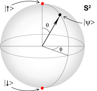
Figure 1: Isomorphism between the state space $\mathbb{P}^{1}$ of a spin-$\textstyle\frac{1}{2}$ system and the two-sphere $\mathbb{S}^{2}$. A state $|\psi\rangle$ in $\mathbb{P}^{1}$ corresponds to a point on $\mathbb{S}^{2}$ and hence can be expressed in the form $|\psi\rangle\!=\!\cos\mbox{$\textstyle\frac{1}{2}$}\,\theta{|\!\uparrow\rangle}+\sin\mbox{$\textstyle\frac{1}{2}$}\,\theta\,\mbox{$\rm e$}^{{\rm i}\phi}{|\!\downarrow\rangle}$. Since a two-sphere $\mathbb{S}^{2}$ can be embedded in $\mathbb{R}^{3}$, we can use the isomorphism $\mathbb{P}^{1}\sim\mathbb{S}^{2}$ to identify the north pole of the sphere as the $S_{z}=\frac{1}{2}$ ‘up’ state ${|\!\uparrow\rangle}$, and the south pole as the $S_{z}=-\frac{1}{2}$ ‘down’ state ${|\!\downarrow\rangle}$. This relation in quantum mechanics is called the Pauli correspondence. Hence we can associate spin directions with points in the state space.

A general pure state can be represented by spherical coordinates on $\mathbb{S}^{2}$, as shown in Figure 1. We can then use a two-component spinor notation for quantum states. Letting the spinor $\psi^{A}$, $A=0,1$, represent a point on $\mathbb{P}^{1}$, we relate this to the corresponding point on $\mathbb{S}^{2}$ by writing

$$\psi^{A}=\left(\cos\mbox{$\textstyle\frac{1}{2}$}\,\theta\,,\ \ \sin\mbox{$\textstyle\frac{1}{2}$}\,\theta\,\mbox{$\rm e$}^{{\rm i}\phi}\right)\qquad(0\leq\theta\leq\pi,\ 0\leq\phi<2\pi).$$ (4)

We let $\alpha^{A}=(1,\,0)$ represent the spin-up state (the north pole on $\mathbb{S}^{2}$, for which $\theta=0$), and $\bar{\alpha}^{A}=\epsilon^{AB}\bar{\alpha}_{B}=(0,\,1)$ the spin down state, where $\epsilon^{AB}$ is the anti-symmetric spinor and ${\bar{\alpha}}_{B}$ is the complex conjugate of $\alpha^{B}$. We use $\alpha^{A}$ and $\bar{\alpha}^{A}$ as our basis in $\mathbb{P}^{1}$ and express the general pure state as $\psi^{A}=u\alpha^{A}+v\bar{\alpha}^{A}$, where $(u,v)$ are the homogeneous coordinates of that point.

3 Two-qubit entanglement

How is quantum entanglement represented in geometric terms? If one system is represented by the Hilbert space ${\mathbb{C}}^{n+1}$, and another by ${\mathbb{C}}^{m+1}$, then the combined system is represented by the tensor product ${\mathbb{C}}^{n+1}\otimes{\mathbb{C}}^{m+1}$. Projectively, the state spaces are given, respectively, by $\mathbb{P}^{n}$ and $\mathbb{P}^{m}$, while the state space of the combined system is $\mathbb{P}^{(n+1)(m+1)-1}$. A characteristic feature of complex projective space is that it admits what is called the Segré embedding: $\mathbb{P}^{n}\times\mathbb{P}^{m}\hookrightarrow\mathbb{P}^{(n+1)(m+1)-1}$. The product space $\mathbb{P}^{n}\times\mathbb{P}^{m}$ for the disentangled quantum states thus ‘lives’ inside the large state space.

We consider the state space $\mathbb{P}^{3}$ of a pair of entangled spin-$\textstyle\frac{1}{2}$ particles (the two-qubit system), and represent a generic state by a spinor $\psi^{AB}$. The disentangled states lie on the ruled surface $\mathbb{P}^{1}\times\mathbb{P}^{1}\subset\mathbb{P}^{3}$, which is the quadric surface $\mathcal{Q}$ given by the solution to the equation $\epsilon_{AC}\epsilon_{BD}\psi^{AB}\psi^{CD}=0$. States on $\mathcal{Q}$ are of the form $\psi^{AB}=\psi^{A}_{1}\psi^{B}_{2}$ where each of the spinors $\psi^{A}_{1}$ and $\psi^{B}_{2}$ describes one of the spin-$\textstyle\frac{1}{2}$ particles. The two spinors need not be the same, and we are free to measure the two spins in different directions. Hence for the disentangled two-particle states we can write

$$\psi_{1}^{A}=\left(\cos\mbox{$\textstyle\frac{1}{2}$}\,\theta_{1},\ \ \sin\mbox{$\textstyle\frac{1}{2}$}\,\theta_{1}\,\mbox{$\rm e$}^{{\rm i}\phi_{1}}\right)\quad{\rm and}\quad\psi_{2}^{A}=\left(\cos\mbox{$\textstyle\frac{1}{2}$}\,\theta_{2},\ \ \sin\mbox{$\textstyle\frac{1}{2}$}\,\theta_{2}\,\mbox{$\rm e$}^{{\rm i}\phi_{2}}\right).$$ (5)

Here $(\theta_{k},\phi_{k})$ fix the spin directions of particles $k=1,2$ on the corresponding Bloch balls.

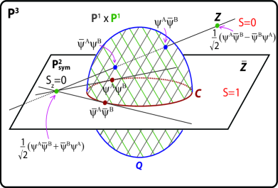
Figure 2: The state space of two spin-$\textstyle\frac{1}{2}$ particles. The disentangled states form a ruled surface ${\mathcal{Q}}=\mathbb{P}^{1}\times\mathbb{P}^{1}$. The singlet state $Z$ in $\mathbb{P}^{3}$ is invariant under local unitary transformations. Its conjugate $\bar{Z}$ is the plane $\mathbb{P}^{2}$ of totally symmetric states, and is spanned by the triplet states given by $S_{z}=0,\pm 1$. The intersection of ${\mathcal{Q}}$ and ${\bar{Z}}$ is a conic ${\mathcal{C}}$. The line joining the singlet state and the spin-$0$ triplet state intersects ${\mathcal{Q}}$ at two points corresponding to $|\!\uparrow\downarrow\rangle$ and $|\!\downarrow\uparrow\rangle$.

If the system is in a state of total spin zero, it is given by the totally antisymmetric singlet $Z$ expressible in the form $\psi^{AB}=\frac{1}{\surd 2}\epsilon^{AB}$. The conjugate of the singlet state is the plane $\mathbb{P}^{2}_{\rm sym}$ of totally symmetric states. The triplet states with $S^{2}=1$ and $S_{z}=1,0,-1$ lie on $\mathbb{P}^{2}_{\rm sym}$ (see Figure 2). The plane of symmetric states intersects the quadric in a conic curve $\mathcal{C}=\mathcal{Q}\cap\mathbb{P}^{2}_{\rm sym}$. The conic is generated by a Veronese embedding of $\mathbb{P}^{1}$ in $\mathbb{P}^{2}_{\rm sym}$, in such a way that the Pauli correspondence for the spin directions in ${\mathbb{R}}^{3}$ is induced in the state space of higher spins. Each point on $\mathcal{C}$ represents a spin-one state $\psi^{AB}$ for some direction $(\theta,\phi)$ in ${\mathbb{R}}^{3}$. Thus $\mathcal{C}$ has the topology ${\mathbb{S}}^{2}$. The choice of the spin direction fixes the $S_{z}=1$ triplet state $\psi^{AB}=\psi^{A}\psi^{B}$. Its complex conjugate is a line which is tangent to the conic at $\psi^{AB}=\bar{\psi}^{A}\bar{\psi}^{B}$, corresponding to the $S_{z}=-1$ state. The intersection of the conjugate lines of the two states $S_{z}=\pm 1$ gives the $S_{z}=0$ state $\psi^{AB}=\frac{1}{\surd 2}(\psi^{A}\bar{\psi}^{B}+\bar{\psi}^{B}\psi^{A})$.

If the system is initially in the singlet state $Z$, or, more generally, in a superposition of the singlet state and the $S_{z}=0$ triplet state, there are two disentangled states that can result as a consequence of a spin measurement along the $z$-axis for one of the particles. These can be formed by connecting the singlet state and the $S_{z}=0$ triplet state with a line. This line intersects the quadric in two points $\psi^{AB}=\psi^{A}\bar{\psi}^{B}$ and $\psi^{AB}=\bar{\psi}^{A}\psi^{B}$, which are the possible results of a spin measurement.

4 Three-qubit entanglement

The geometry of the three-qubit system is very rich. The state space $\mathbb{P}^{7}$ of the three-qubit system is obtained by projecting the tensor product space ${\mathbb{C}}^{2}\otimes{\mathbb{C}}^{2}\otimes{\mathbb{C}}^{2}$. There are several different types of entanglement that can result [4]. First, we have the completely disentangled states. These constitute a triply-ruled three-surface $\mathcal{D}=\mathbb{P}^{1}\times\mathbb{P}^{1}\times\mathbb{P}^{1}$. Next, we have the partly entangled states, where one of the particles is disentangled from the other two. There are three such systems of partly entangled states, each of which constitutes a four-dimensional variety $Q_{i}\subset{\mathbb{P}}^{7}$ ($i=1,2,3$) with the structure of $\mathbb{P}^{1}\times\mathbb{P}^{3}$. The ${\mathbb{P}}^{1}$ in each case represents the state space of the disentangled particle, and the ${\mathbb{P}}^{3}$ represents the state space of the remaining entangled pair. It should be evident that $\mathcal{D}=Q_{1}\cap Q_{2}\cap Q_{3}$. Finally, we have the states for which all three particles are entangled. Figure 3 shows a schematic illustration of $\mathbb{P}^{7}$, highlighting the totally disentangled and partially entangled state spaces.

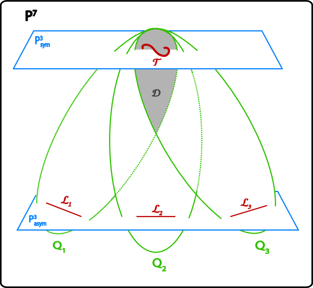
Figure 3: The state space of three spin-$\textstyle\frac{1}{2}$ particles. There are three configurations of partly entangled states $\{Q_{i}\}_{i=1,2,3}$. Their intersection is the space of totally disentangled states $\mathcal{D}$. The symmetric states form a hyperplane $\mathbb{P}^{3}_{\rm sym}$ whose orthogonal complement $\mathbb{P}^{3}_{\rm asym}$ intersects each $Q_{i}$ in a line $\mathcal{L}_{i}$. The line ${\mathcal{L}}_{i}$ represents for each $i$ the state space of particle $i$ when the two remaining particles are entangled to form an $S=0$ singlet.

The states of total spin $S=\frac{3}{2}$ form a hyperplane ${\mathbb{P}}^{3}_{\rm sym}\subset{\mathbb{P}}^{7}$. These states are represented by totally symmetric spinors, i.e. those satisfying $\psi^{ABC}=\psi^{(ABC)}$, where the round brackets denote symmetrisation. The states of total spin $S=\frac{1}{2}$ also constitute a hyperplane of dimension three, which we call ${\mathbb{P}}^{3}_{\rm asym}$. The ‘asymmetric’ states are those that are of the form

$$\psi^{ABC}=\alpha^{A}\epsilon^{BC}+\beta^{B}\epsilon^{CA}+\gamma^{C}\epsilon^{AB}$$ (6)

for some $\alpha^{A},\beta^{A},\gamma^{A}$. It should be evident that the symmetric states and the asymmetric states are orthogonal. Thus ${\mathbb{P}}^{3}_{\rm asym}$ is the orthogonal complement of ${\mathbb{P}}^{3}_{\rm sym}$ in ${\mathbb{P}}^{7}$.

The hyperplane ${\mathbb{P}}^{3}_{\rm sym}$ intersects ${\mathcal{D}}$ in a twisted cubic curve $\mathcal{T}=\mathbb{P}^{3}_{{\rm sym}}\cap\mathcal{D}$. See [5] for the properties of the twisted cubic. This curve is given by the Veronese embedding of $\mathbb{P}^{1}$ in $\mathbb{P}^{3}_{\rm sym}$, which takes the form $\psi^{A}\to\psi^{A}\psi^{B}\psi^{C}$ (see, e.g., references [2, 6]). The Veronese embedding induces the Pauli correspondence in the state space $\mathbb{P}^{7}$. In particular, if $S=\frac{3}{2}$, then we have a quadruplet of possible spin states relative to the $z$-axis, with $S_{z}=\mbox{$\textstyle\frac{3}{2}$},\mbox{$\textstyle\frac{1}{2}$},-\mbox{$\textstyle\frac{1}{2}$},-\mbox{$\textstyle\frac{3}{2}$}$. The hyperplane $\mathbb{P}^{3}_{{\rm sym}}$ is spanned by $S=\mbox{$\textstyle\frac{3}{2}$}$ quadruplet. In particular, the $S_{z}=\mbox{$\textstyle\frac{3}{2}$}$ and $S_{z}=-\mbox{$\textstyle\frac{3}{2}$}$ states lie on $\mathcal{T}$. If the spinor $\psi^{A}$ has $S_{z}=\frac{1}{2}$, then the $S_{z}=\mbox{$\textstyle\frac{3}{2}$}$ and $S_{z}=-\mbox{$\textstyle\frac{3}{2}$}$ states are given by $\psi^{ABC}=\psi^{A}\psi^{B}\psi^{C}$ and $\psi^{ABC}=\bar{\psi}^{A}\bar{\psi}^{B}\bar{\psi}^{C}$, respectively.

The tangent line to a point $\alpha^{A}\alpha^{B}\alpha^{C}$ on ${\mathcal{T}}$ consists of spinors of the form $\psi^{ABC}=\alpha^{(A}\alpha^{B}x^{C)}$ for some $x^{A}$. The so-called osculating 2-plane at $\alpha^{A}\alpha^{B}\alpha^{C}$ consists of spinors of the form $\psi^{ABC}=\alpha^{(A}x^{B}y^{C)}$ for some $x^{A},y^{A}$. Clearly, the tangent line lies on the osculating plane. The two-dimensional envelope generated by the tangent lines to ${\mathcal{T}}$ generates a quartic surface ${\mathcal{H}}_{\rm sym}$ in ${\mathbb{P}}^{3}_{\rm sym}$, given by the equation $Q_{AB}Q^{AB}=0$, where $Q_{AB}=\psi_{A}^{\ CD}\psi_{BCD}$ and $\psi^{ABC}=\psi^{(ABC)}$. The states of ${\mathbb{P}}^{3}_{\rm sym}$ are of three types: those on ${\mathcal{T}}$; those on ${\mathcal{H}}_{\rm sym}\backslash{\mathcal{T}}$; and those on ${\mathbb{P}}^{3}_{\rm sym}\backslash{\mathcal{H}}_{\rm sym}$. The complex conjugate of a point $\psi^{A}\psi^{B}\psi^{C}$ on $\mathcal{T}$ is a six-dimensional hyperplane in $\mathbb{P}^{7}$, which intersects $\mathbb{P}^{3}_{{\rm sym}}$ at the osculating plane of the point ${\bar{\psi}}^{A}{\bar{\psi}}^{B}{\bar{\psi}}^{C}$ on $\mathcal{T}$. As illustrated in Figure 4, the intersection of the tangent line of $\mathcal{T}$ at the $S_{z}=\mbox{$\textstyle\frac{3}{2}$}$ state and the osculating plane of $\mathcal{T}$ at the $S_{z}=-\mbox{$\textstyle\frac{3}{2}$}$ state is the $S_{z}=\frac{1}{2}$ state $\frac{1}{\surd 3}(\psi^{A}\psi^{B}\bar{\psi}^{C}+\psi^{A}\bar{\psi}^{B}\psi^{C}+\bar{\psi}^{A}\psi^{B}\psi^{C})$. Similarly, the $S_{z}=-\frac{1}{2}$ state $\frac{1}{\surd 3}(\psi^{A}\bar{\psi}^{B}\bar{\psi}^{C}+\bar{\psi}^{A}\psi^{B}\bar{\psi}^{C}+\bar{\psi}^{A}\bar{\psi}^{B}\psi^{C})$ is the intersection of tangent line of $\mathcal{T}$ at the $S_{z}=-\mbox{$\textstyle\frac{3}{2}$}$ state and the osculating plane of $\mathcal{T}$ at the $S_{z}=\mbox{$\textstyle\frac{3}{2}$}$ state.

The space $\mathbb{P}^{3}_{\rm asym}$ intersects each of the varieties $\{Q_{i}\}_{i=1,2,3}$ in a line $\mathcal{L}_{i}=Q_{i}\cap\mathbb{P}^{3}_{\rm asym}$. These lines represent the singlet states of the entangled pairs in the $\{Q_{i}\}$. This follows because the states of $\mathbb{P}^{3}_{{\rm asym}}$ can be expressed in the form $\alpha^{A}\epsilon^{BC}+\beta^{B}\epsilon^{CA}+\gamma^{C}\epsilon^{AB}$. The intersection of $\mathbb{P}^{3}_{{\rm asym}}$ with $Q_{1}$ thus takes the form $\alpha^{A}\epsilon^{BC}$, where $\alpha^{A}\in\mathbb{P}^{1}$ and $\epsilon^{BC}\in\mathbb{P}^{3}$. Since $\epsilon^{BC}$ is antisymmetric, it corresponds to the singlet state in $\mathbb{P}^{3}$. Then as $\alpha^{A}$ varies, we obtain the ‘singlet’ line $\mathcal{L}_{1}$. This configuration is illustrated in Figure 3.

An interesting feature of 3-qubit entanglement is that under stochastic local operations and classical communication (SLOCC) operations there are six different equivalence classes of entanglement [7]. The SLOCC operations are elements of the group $SL(2,\mathbb{C})^{\otimes 3}$. The space of equivalence classes is then $\mathbb{C}^{2}\otimes\mathbb{C}^{2}\otimes\mathbb{C}^{2}/SL(2,\mathbb{C})^{\otimes 3}$. Two states are equivalent under SLOCC if there exists an invertible local operation interpolating them. The six classes are the totally disentangled states, the three configurations of partly entangled states, and the two different classes of totally entangled states: those that are locally equivalent to the Greenberger-Horne-Zeilinger state $|{\rm GHZ}\rangle=\frac{1}{\surd 2}(\psi^{A}\psi^{B}\psi^{C}+\bar{\psi}^{A}\bar{\psi}^{B}\bar{\psi}^{C})$, and those locally equivalent to the Werner state $|{\rm W}\rangle=\frac{1}{\surd{3}}(\psi^{A}\psi^{B}\bar{\psi}^{C}+\psi^{A}\bar{\psi}^{B}\psi^{C}+\bar{\psi}^{A}\psi^{B}\psi^{C})$.

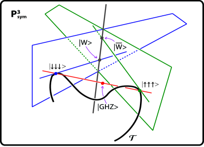
Figure 4: A close up of the hyperplane $\mathbb{P}^{3}_{{\rm sym}}$ of symmetric states. The twisted cubic $\mathcal{T}$ is the intersection between this hyperplane and the space of totally disentangled states $\mathcal{D}$. For every spin direction the states ${|\!\uparrow\uparrow\uparrow\rangle}$ and ${|\!\downarrow\downarrow\downarrow\rangle}$ lie on the twisted cubic. The GHZ state $|\textrm{GHZ}\rangle=\frac{1}{\surd 2}({|\!\uparrow\uparrow\uparrow\rangle}+{|\!\downarrow\downarrow\downarrow\rangle})$ is found on the line joining them, and the $S_{z}=\frac{1}{2}$ Werner state $|\textrm{W}\rangle=\frac{1}{\surd{3}}({|\!\uparrow\uparrow\downarrow\rangle}+{|\!\uparrow\downarrow\uparrow\rangle}+{|\!\downarrow\uparrow\uparrow\rangle})$ is given by the intersection of the osculating plane at ${|\!\uparrow\uparrow\uparrow\rangle}$ and the tangent line at ${|\!\downarrow\downarrow\downarrow\rangle}$.

The GHZ state is symmetric and lies on the chord that joins the two quadruplet states that lie on the twisted cubic. The GHZ state is usually said to be the maximally entangled state, in the sense that it maximally violates the Bell inequalities. If one of the particles is disentangled from the rest, however, then the other two are automatically disentangled. The W state on the other hand maximises 2-qubit entanglement inside the 3-qubit state, so that if one of the particles is disentangled it leaves the other two maximally entangled. The ‘three-tangle’ $4|{\rm Det}(\psi)|$, where ${\rm Det}(\psi)$ is the Cayley hyperdeterminant [8], is zero for all states except those states that are equivalent to the GHZ state (see [9, 10]). The idea is as follows. We consider the space ${\mathcal{D}}$ of totally disentangled states, and let ${\mathcal{H}}$ denote the six-dimensional variety generated by the system of 3-hyperplanes tangent to ${\mathcal{D}}$. Then ${\mathcal{H}}$ turns out to be a quartic surface in ${\mathbb{P}}^{7}$, consisting of those points for which the Cayley invariant vanishes. In particular, ${\mathcal{H}}$ is given by

$$\psi_{A}^{\ BC}\psi_{BCD}\psi_{P}^{\ RS}\psi_{QRS}\epsilon^{AP}\epsilon^{BQ}=0.$$ (7)

A necessary and sufficient condition for $\psi^{ABC}$ to satisfy this relation is that

$$\psi^{ABC}=x^{A}\beta^{B}\gamma^{C}+\alpha^{A}y^{B}\gamma^{C}+\alpha^{A}\beta^{B}z^{C}$$ (8)

for some $\alpha^{A},\beta^{B},\gamma^{C},x^{A},y^{B},z^{C}$. In particular, if $\alpha^{A}\beta^{B}\gamma^{C}$ is a point in ${\mathcal{D}}$, then the tangent plane to ${\mathcal{D}}$ at that point consists of states of the form (8) for some choice of $x^{A},y^{B},z^{C}$. On the other hand, under the SLOCC classification, the states that are equivalent to the GHZ state have nonzero hyperdeterminant. This can be seen from the fact that the GHZ state lies on a chord of ${\mathcal{T}}$. In particular, we note that ${\mathcal{H}}_{\rm sym}={\mathcal{H}}\cap{\mathbb{P}}^{3}_{\rm sym}$.

There are other open questions in describing entanglement, both geometrically and algebraically. For example, is there a geometrically unambiguous measure of pure-state entanglement for the 3-qubit system? If so, can it be extended to $n$-qubits for $n\geq 4$? Right now there is an active search being undertaken to find a good way of quantifying the amount of entanglement in a quantum state. We hope a geometric formulation will provide intuitive answers to these questions.

DCB acknowledges support from The Royal Society. ACTG would like to thank the organisers of the DICE2006 conference in Piombino, Italy, 11-15 September 2006 for the opportunity to present this work.

References

• [1] T. W. B. Kibble 1979 Geometrization of quantum mechanics, Commun. Math. Phys., 65, 189-201
• [2] D. C. Brody & L. P. Hughston 2001 Geometric quantum mechanics, J. Geom. Phys. 38, 19-53
• [3] L. P. Hughston 1995 Geometric aspects of quantum mechanics, in Twistor Theory, Huggett, S., ed., (New York: Marcel Dekker)
• [4] S. Ferrando i Margalet 2000 Geometric aspects of quantum theory, MSc Thesis, Department of Mathematics, King’s College London
• [5] P. W. Wood 1960 The twisted cubic, with some account of the metrical properties of the cubical hyperbola (New York: Hafner Publishing Co.)
• [6] M. G. Eastwood, L. P. Hughston & T.R. Hurd 1979 Massless fields based on a twisted cubic. In Advances in Twistor Theory, L.P. Hughston & R.S.Ward, eds. (London: Pitman)
• [7] W. Dur, G. Vidal & J. I. Cirac 2000 Three qubits can be entangled in two inequivalent ways, Phys. Rev. A62, 062314
• [8] I. M. Gelfand, M. M. Kapranov, & A. V. Zelevinsky 1994 Discriminants, Resultants, and Multidimensional Determinants (Basel: Birkhäuser)
• [9] A. Miyake 2003 Classification of multipartite entangled states by multidimensional determinants, Phys. Rev. A 67, 012108
• [10] P. Lévay 2005 Geometry of three-qubit entanglement, Phys. Rev. A71, 012334