On the Impossibility of a Quantum Sieve Algorithm for Graph Isomorphism

Abstract.

It is known that any quantum algorithm for Graph Isomorphism that works within the framework of the hidden subgroup problem (HSP) must perform highly entangled measurements across $\Omega(n\log n)$ coset states. One of the only known models for how such a measurement could be carried out efficiently is Kuperberg’s algorithm for the HSP in the dihedral group, in which quantum states are adaptively combined and measured according to the decomposition of tensor products into irreducible representations. This “quantum sieve” starts with coset states, and works its way down towards representations whose probabilities differ depending on, for example, whether the hidden subgroup is trivial or nontrivial.

In this paper we show that no such approach can produce a polynomial-time quantum algorithm for Graph Isomorphism. Specifically, we consider the natural reduction of Graph Isomorphism to the HSP over the the wreath product $S_{n}\wr\mathbb{Z}_{2}$. Using a recently proved bound on the irreducible characters of $S_{n}$, we show that no algorithm in this family can solve Graph Isomorphism in less than $e^{\Omega(\sqrt{n})}$ time, no matter what adaptive rule it uses to select and combine quantum states. In particular, algorithms of this type can offer essentially no improvement over the best known classical algorithms, which run in time $e^{O(\sqrt{n\log n})}$.

1. Introduction

The discovery of Shor’s and Simon’s algorithms began a frenzied charge to uncover the full algorithmic potential of a general purpose quantum computer. Creative invocations of the order-finding primitive yielded efficient quantum algorithms for a number of other number-theoretic problems [Hal02, Hal05]. As the field matured, these algorithms were roughly unified under the general framework of the hidden subgroup problem, where one must determine a subgroup $H$ of a group $G$ by querying an oracle $f:G\rightarrow S$ known to have the property that $f(g)=f(gh)\Leftrightarrow h\in H$. Solutions to this general problem are the foundation for almost all known superpolynomial speedups offered by quantum algorithms over their classical counterparts (see [AJL06] for an important exception).

The algorithms of Simon and Shor essentially solve the hidden subgroup problem on abelian groups, namely $\mathbb{Z}_{2}^{n}$ and $\mathbb{Z}_{n}^{*}$ respectively. Since then, non-abelian hidden subgroup problems have received a great deal of attention (e.g. [HRTS00, GSVV01, FIM⁺03, MRS04, BCvD05, HMR⁺06]). A major motivation for this work is the fact that we can reduce Graph Isomorphism for rigid graphs of size $n$ to the case of the hidden subgroup problem over the symmetric group $S_{2n}$, or more specifically the wreath product $S_{n}\wr\mathbb{Z}_{2}$, where the hidden subgroup is promised to be either trivial or of order two. The standard approach to these problems is to prepare “coset states” of the form

$$\rho_{H}=\frac{1}{|G|}\sum_{c}\left|cH\right\rangle\left\langle cH\right|\enspace,$$

where $\left|S\right\rangle$, for a subset $S\subset G$, denotes the uniform superposition $(1/\sqrt{|S|})\sum_{g\in S}\left|g\right\rangle$. In the abelian case, one proceeds by computing the quantum Fourier transform of such coset states, measuring the resulting states, and appropriately interpreting the results. In the case of the symmetric group, however, determining $H$ from a quantum measurement of coset states is far more difficult. In particular, no product measurement (that is, a measurement which treats each coset state independently) can efficiently determine a hidden subgroup over $S_{n}$ [MRS05]; in fact, any successful measurement must be entangled over $\Omega(n\log n)$ coset states at once [HMR⁺06].

One of the few proposed methods for building such an entangled measurement comes from Kuperberg’s algorithm for the hidden subgroup problem in the dihedral group [Kup05]. It starts by generating a large number of coset states and subjecting each one to weak Fourier sampling, so that it lies inside a known irreducible representation. It then proceeds with an adaptive “sieve” process, at each step of which it judiciously selects pairs of states and measures them in a basis consistent with the Clebsch-Gordan decomposition of their tensor product into irreducible representations. This sieve continues until we obtain a state lying in an “informative” representation: namely, one from which information about the hidden subgroup can be easily extracted. We can visualize a run of the sieve as a forest, where leaves consist of the initial coset states, each internal node measures the tensor product of its parents, and the informative representations lie at the roots.

This approach is especially attractive in cases like Graph Isomorphism, where all we need to know is whether the hidden subgroup is trivial or nontrivial. Specifically, suppose that the hidden subgroup $H$ is promised to be either the trivial subgroup $\{1\}$ or a conjugate of a known subgroup $H_{0}$. Assume further that there is an irreducible representation $\sigma$ of $G$ with the property that $\sum_{h\in H_{0}}\sigma(h)=0$; that is, a “missing harmonic” in the sense of [MR05a]. In this case, if $H$ is nontrivial then the probability of observing $\sigma$ under weak Fourier sampling of the coset state $\rho_{H}$ is zero. More generally, as we discuss below, the irrep $\sigma$ cannot appear at any time in the sieve. If, on the other hand, one can guarantee that the sieve does observe $\sigma$ with significant probability when the hidden subgroup is trivial and the corresponding states are completely mixed, it gives us an algorithm to distinguish the two cases.

For example, if we consider the case of the hidden subgroup problem in the dihedral group $D_{n}$ where $H$ is either trivial or a conjugate of $H_{0}=\{1,m\}$ where $m$ is an involution, then the sign representation $\pi$ is a missing harmonic. Applying Kuperberg’s sieve, we observe $\pi$ with significant probability after $e^{O(\sqrt{n})}$ steps if $H$ is trivial, while we can never observe it if $H$ is of order $2$. A similar approach was applied to groups of the form $G^{n}$ by Alagić et al. [AMR06].

We show here, however, that the hidden subgroup problem related to Graph Isomorphism cannot be solved efficiently by any algorithm in this family. Specifically, no matter what adaptive selection rule it uses to choose pairs of states to combine and measure, such a sieve cannot distinguish the isomorphic and nonisomorphic cases unless it takes $e^{\Omega(\sqrt{n})}$ time (and uses this many coset states). In comparison, the best known classical algorithms for Graph Isomorphism run in time $e^{O(\sqrt{n\log n})}$ for general graphs [Bab80, Bab83] and $e^{O(n^{1/3}\log^{2}n)}$ for strongly regular graphs [Spi96]. Therefore, quantum algorithms of this kind can offer no meaningful improvement over their classical counterparts.

Our proof relies on several ingredients. First, we give a formal definition of quantum sieve algorithms, and we derive a combinatorial description of the probability distributions of their observations in the trivial and nontrivial cases. We then focus on the case where the ambient group is a wreath product $G\wr\mathbb{Z}_{2}$, and show that no information is gained until the sieve observes a so-called inhomogeneous representation. Then, in the case where $G=S_{n}$, we rely on a bound on the characters of the symmetric group proved very recently by Rattan and Śniady [RŚ06] to show that the total variation distance between the trivial and nontrivial cases is at most $e^{-b\sqrt{n}}$ unless the sieve takes $e^{a\sqrt{n}}$ time, for some constants $a,b>0$.

We note that two of the present authors gave this result in conditional form in [MR06], in which they presented a conjectured bound on the characters of $S_{n}$. Indeed, it was this conjecture which inspired the work of [RŚ06] who proved its weaker version, which, along with some additional arguments, allows us to prove the results of [MR06] unconditionally.

We refer the reader to [Ser77, JK81] for an introduction to to the representation theory of finite groups, and in particular of the symmetric group $S_{n}$. One fact which we use repeatedly is that the $\tau$-isotypic subspace, i.e., the subspace of a representation $\sigma$ which consists of copies of an irrep $\tau$, is the image of the projection operator

$$\Pi_{\tau}=\frac{1}{|G|}\sum_{g\in G}d_{\tau}\chi_{\tau}(g)^{*}\sigma(g)\enspace.$$

These projection operators can be combined to create a measurement whose outcomes are names of irreducible representations. Applying such a measurement to coset states is known as weak Fourier sampling; we use the term isotypic sampling to refer to the more general case of applying an arbitrary group action to a multiregister state.

2. Fourier analysis on finite groups

In this section we review the representation theory of finite groups. Our treatment is primarily for the purposes of setting down notation; we refer the reader to [Ser77] for a complete account. Let $G$ be a finite group. A representation $\sigma$ of $G$ is a homomorphism $\sigma:G\to\textsf{U}(V)$, where $V$ is a finite-dimensional Hilbert space and $\textsf{U}(V)$ is the group of unitary operators on $V$. The dimension of $\sigma$, denoted $d_{\sigma}$, is the dimension of the vector space $V$. Fixing a representation $\sigma:G\to\textsf{U}(V)$, we say that a subspace $W\subset V$ is invariant if $\sigma(g)\cdot W=W$ for all $g\in G$. When $\sigma$ has no invariant subspaces other than the trivial subspace $\{\mathbf{0}\}$ and $V$ itself, $\sigma$ is said to be irreducible.

If two representations $\sigma$ and $\sigma^{\prime}$ are the same up to a unitary change of basis, we say that they are equivalent. It is a fact that any finite group $G$ has a finite number of distinct irreducible representations up to equivalence and, for a group $G$, we let $\widehat{G}$ denote a set of representations containing exactly one from each equivalence class. We often say that each $\sigma\in\widehat{G}$ is the name of an irreducible representation, or an irrep for short.

The irreps of $G$ give rise to the Fourier transform. Specifically, for a function $f:G\to\mathbb{C}$ and an element $\sigma\in\widehat{G}$, define the Fourier transform of $f$ at $\sigma$ to be

$$\hat{f}(\sigma)=\sqrt{\frac{d_{\sigma}}{|G|}}\sum_{g\in G}f(g)\sigma(g)\enspace.$$

The leading coefficients are chosen to the make the transform unitary, so that it preserves inner products:

$$\langle f_{1},f_{2}\rangle=\sum_{g}f_{1}^{*}(g)f_{2}(g)=\sum_{\sigma\in\widehat{G}}\operatorname{\textbf{tr}}\!\left(\hat{f_{1}}(\sigma)^{\dagger}\cdot\hat{f_{2}}(\sigma)\right)\enspace.$$

If $\sigma$ is not irreducible, it can be decomposed into a direct sum of irreps $\tau_{i}$, each of which acts on an invariant subspace, and we write $\sigma\cong\tau_{1}\oplus\cdots\oplus\tau_{k}$. In general, a given $\tau$ can appear multiple times in this decomposition, in the sense that $\sigma$ may have an invariant subspace isomorphic to the direct sum of $a_{\tau}$ copies of $\tau$. In this case $a_{\tau}$ is called the multiplicity of $\tau$ in the decomposition of $\sigma$.

There is a natural product operation on representations: if $\lambda:G\to\textsf{U}(V)$ and $\mu:G\to\textsf{U}(W)$ are representations of $G$, we may define a new representation $\lambda\otimes\mu:G\to\textsf{U}(V\otimes W)$ as $(\lambda\otimes\mu)(g):\mathbf{u}\otimes\mathbf{v}\mapsto\lambda(g)\mathbf{u}\otimes\mu(g)\mathbf{v}$. This representation corresponds to the diagonal action of $G$ on $V\otimes W$, in which we apply the same group element to both parts of the tensor product. In general, the representation $\lambda\otimes\mu$ is not irreducible, even when both $\lambda$ and $\mu$ are. This leads to the Clebsch-Gordan problem, that of decomposing $\lambda\otimes\mu$ into irreps.

Given a representation $\sigma$ we define the character of $\sigma$, denoted $\chi_{\sigma}$, to be the trace $\chi_{\sigma}(g)=\operatorname{\textbf{tr}}\sigma(g)$. As the trace of a linear operator is invariant under conjugation, characters are constant on the conjugacy classes of $G$. Characters are a powerful tool for reasoning about the decomposition of reducible representations. In particular, when $\sigma=\bigoplus_{i}\tau_{i}$ we have $\chi_{\sigma}=\sum_{i}\chi_{\tau_{i}}$ and, moreover, for $\sigma,\tau\in\widehat{G}$, we have the orthogonality conditions

$$\left\langle\chi_{\sigma},\chi_{\tau}\right\rangle_{G}=\frac{1}{|G|}\sum_{g\in G}\chi_{\sigma}(g)\chi_{\tau}(g)^{*}=\begin{cases}1&\sigma=\tau\enspace,\\ 0&\sigma\neq\tau\enspace.\end{cases}$$

Therefore, given a representation $\sigma$ and an irrep $\tau$, the multiplicity $a_{\tau}$ with which $\tau$ appears in the decomposition of $\sigma$ is $\left\langle\chi_{\tau},\chi_{\sigma}\right\rangle_{G}$. For example, since $\chi_{\lambda\otimes\mu}(g)=\chi_{\lambda}(g)\cdot\chi_{\mu}(g)$, the multiplicity of $\tau$ in the Clebsch-Gordan decomposition of $\lambda\otimes\mu$ is $\left\langle\chi_{\tau},\chi_{\lambda}\chi_{\mu}\right\rangle_{G}$.

A representation $\sigma$ is said to be isotypic if the irreducible factors appearing in the decomposition are all isomorphic, which is to say that there is a single nonzero $a_{\tau}$ in the decomposition above. Any representation $\sigma$ may be uniquely decomposed into maximal isotypic subspaces, one for each irrep $\tau$ of $G$; these subspaces are precisely those spanned by all copies of $\tau$ in $\sigma$. In fact, for each $\tau$ this subspace is the image of an explicit projection operator $\Pi_{\tau}$ which can be written as

$$\Pi_{\tau}=\frac{1}{|G|}\sum_{g\in G}d_{\tau}\chi_{\tau}(g)^{*}\sigma(g)\enspace.$$

A useful fact is that $\Pi_{\tau}$ commutes with the group action; that is, for any $h\in G$ we have

$$\sigma(h)\Pi_{\tau}\sigma(h)^{\dagger}=\frac{1}{|G|}\sum_{g\in G}d_{\tau}\chi_{\tau}(g)^{*}\sigma(hgh^{-1})=\\ \frac{1}{|G|}\sum_{g\in G}d_{\tau}\chi_{\tau}(h^{-1}gh)^{*}\sigma(g)=\frac{1}{|G|}\sum_{g\in G}d_{\tau}\chi_{\tau}(g)^{*}\sigma(g)=\Pi_{\tau}\enspace.$$

Our algorithms will perform measurements which project into these maximal isotypic subspaces and observe the resulting irrep name $\tau$. For the particular case of coset states, this measurement is called weak Fourier sampling in the literature; however, since we are interested in a more general process which in fact performs a kind of strong multiregister sampling on the original coset states, we will use the term isotypic sampling instead. Finally, we discuss the structure of a specific representation, the (right) regular representation reg, which plays an important role in the analysis below. reg is given by the permutation action of $G$ on itself. Specifically, let $\mathbb{C}[G]$ be the group algebra of $G$; this is the $|G|$-dimensional vector space of formal sums

$$\Bigl{\{}\sum_{g}\alpha_{g}\cdot g\mid\alpha_{g}\in\mathbb{C}\Bigr{\}}\enspace.$$

(Note that $\mathbb{C}[G]$ is precisely the Hilbert space of a single register containing a superposition of group elements.) Then reg is the representation $\textbf{reg}:G\to\textsf{U}(\mathbb{C}[G])$ given by linearly extending right multiplication, $\textbf{reg}(g):h\mapsto hg$. It is not hard to see that its character $\chi_{\textbf{reg}}$ is given by

$$\chi_{\textbf{reg}}(g)=\begin{cases}|G|&g=1\enspace,\\ 0&g\neq 1\enspace,\end{cases}$$

in which case we have $\left\langle\chi_{\textbf{reg}},\chi_{\sigma}\right\rangle_{G}=d_{\sigma}$ for each $\sigma\in\widehat{G}$. Thus reg contains $d_{\sigma}$ copies of each irrep $\sigma\in\widehat{G}$, and counting dimensions on each side of this decomposition implies

(1) $$|G|=\sum_{\sigma\in\widehat{G}}d_{\sigma}^{2}\enspace.$$

This equation suggests a natural probability distribution on $\widehat{G}$, the Plancherel distribution, which assigns to each irrep $\sigma$ the probability ${\mathcal{P}}_{\rm planch}^{G}(\sigma)=d_{\sigma}^{2}/|G|$. This is simply the dimensionwise fraction of $\mathbb{C}[G]$ consisting of copies of $\sigma$; indeed, if we perform isotypic sampling on the completely mixed state on $\mathbb{C}[G]$, or equivalently the coset state where the hidden subgroup is trivial, we observe exactly this distribution.

In general, we can consider subspaces of $\mathbb{C}[G]$ that are invariant under left multiplication, right multiplication, or both; these subspaces are called left-, right-, or bi-invariant respectively. For each $\sigma\in\widehat{G}$, the maximal $\sigma$-isotypic subspace is a $d_{\sigma}^{2}$-dimensional bi-invariant subspace; it can be broken up further into $d_{\sigma}$ $d_{\sigma}$-dimensional left-invariant subspaces, or (transversely) $d_{\sigma}$ $d_{\sigma}$-dimensional right-invariant subspaces. However, this decomposition is not unique. If $\sigma$ acts on a vector space $V$, then choosing an orthonormal basis for $V$ allows us to view $\sigma(g)$ as a $d_{\sigma}\times d_{\sigma}$ matrix. Then $\sigma$ acts on the $d_{\sigma}^{2}$-dimensional space of such matrices by left or right multiplication, and the columns and rows correspond to left- and right-invariant spaces respectively.

3. Clebsch-Gordan sieves

Consider the hidden subgroup problem over a group $G$ with the added promise that the hidden subgroup $H$ is either the trivial subgroup, or a conjugate of some fixed nontrivial subgroup $H_{0}$. We shall consider sieve algorithms for this problem that proceed as follows:

1. The oracle is used to generate $\ell=\ell(n)$ coset states $\rho_{H}$, each of which is subjected to weak Fourier sampling. This results in a set of states $\rho_{i}$, where $\rho_{i}$ is a mixed state known to lie in the $\sigma_{i}$-isotypic subspace of $\mathbb{C}[G]$ for some irrep $\sigma_{i}$.

2. The following combine-and-measure procedure is then repeated as many times as we like. Two states $\rho_{i}$ and $\rho_{j}$ in the set are selected according to an arbitrary adaptive rule that may depend on the entire history of the computation (in existing algorithms of this type, this selection in fact depends only on the irreps $\sigma_{i}$ and $\sigma_{j}$ in which they lie). We then perform isotypic sampling on their tensor product $\rho_{i}\otimes\rho_{j}$: that is, we apply a measurement operator which observes an irrep $\sigma$ in the Clebsch-Gordan decomposition of $\sigma_{i}\otimes\sigma_{j}$ (see [Kup05] or [MR05a] for how this measurement can actually be carried out by applying the diagonal action). This measurement destroys $\rho_{i}$ and $\rho_{j}$, and results in a new mixed state $\rho$ which lies in the maximal $\sigma$-isotypic subspace; we add this new state to the set.

3. Finally, depending on the sequence of observations obtained throughout this process, the algorithm guesses the hidden subgroup.

We set down some notation to discuss the result of applying such an algorithm. Fixing a group $G$ and a subgroup $H$, let $A$ be a sieve algorithm which initially generates $\ell$ coset states. As a bookkeeping tool, we will describe intermediate states of $A$’s progress as a forest of labeled binary trees. Throughout, we will maintain the invariant that the roots of the trees in this forest correspond to the current set of states available to the algorithm.

Initially, the state of the algorithm consists of a forest consisting of $\ell$ single-node trees, each of which is labeled with the irrep name $\sigma_{i}$ that resulted from weak Fourier sampling a coset state, and is associated with the resulting state $\rho_{i}$. Then, each combine-and-measure step selects two root nodes, $r_{1}$ and $r_{2}$, and applies isotypic sampling to the tensor product of their states. We associate the resulting state $\rho$ with a new root node $r$, and place the nodes $r_{1}$ and $r_{2}$ below it as its children. We label this new node with the irrep name $\sigma$ observed in this measurement.

Thus, every node of the forest corresponds to a state that existed at some point during the algorithm, and each node $i$ is labeled with the name of the irrep $\sigma_{i}$ observed in the isotypic measurement performed when that node was created. We call the resulting labeled forest the transcript of the algorithm: note that this transcript contains all the information the algorithm may use to determine the hidden subgroup.

We make several observations about algorithms of this type. First, it is easy to see that nothing is gained by combining $t>2$ states at a time; we can simulate this with an algorithm which builds a binary tree with $t$ leaves, and which ignores the results of all its measurements except the one at the root.

Second, the algorithm maintains the following kind of symmetry under the action of the subgroup $H$. Suppose we have a representation $\sigma$ acting on a Hilbert space $V$. Given a subgroup $H$, we say that a state $\psi\in V$ is $H$-invariant if $\sigma(h)\cdot\psi=\psi$ for all $h\in H$. Similarly, given a mixed state $\rho$, we say that $\rho$ is $H$-invariant if $\sigma(h)\cdot\rho\cdot\sigma(h)^{\dagger}=\rho$ or, equivalently, if $\sigma(h)$ and $\rho$ commute. For instance, the coset state $\rho_{H}$ is $H$-invariant under the right regular representation, since right-multiplying by any $h\in H$ preserves each left coset $cH$. Now, suppose that $\rho_{1}$ and $\rho_{2}$ are $H$-invariant; clearly $\rho_{1}\otimes\rho_{2}$ is $H$-invariant under the diagonal action, and performing isotypic sampling preserves $H$-invariance since $\Pi_{\tau}$ commutes with the action of any group element. Thus the states produced by the algorithm are $H$-invariant throughout.

Third, it is important to note that while at each stage we observe only an irrep name, rather than a basis vector inside that representation, by iterating this process the sieve algorithm actually performs a kind of strong multiregister Fourier sampling on the original set of coset states. For instance, in the dihedral group, suppose that performing weak Fourier sampling on two coset states results in the two-dimensional irreps $\sigma_{j}$ and $\sigma_{k}$, and that we then observe the irrep $\sigma_{j+k}$ under isotypic sampling of their tensor product. We now know that the original coset states were in fact confined to a particular subspace, spanned by two entangled pairs of basis vectors. Finally, we note that the states produced by a sieve algorithm are quite different from coset states. In particular, they belong not to a maximal isotypic subspace of $\mathbb{C}[G]$, but to a (typically much higher-dimensional) non-maximal isotypic subspace of $\mathbb{C}[G]^{\otimes\ell}$, where $\ell$ is the number of coset states feeding into that state (i.e., the number of leaves of the corresponding tree). Moreover, they have more symmetry than coset states, since each isotypic measurement implies a symmetry with respect to the diagonal action on the set of leaves descended from the corresponding internal node. In the next sections we will show how these states can be written in terms of projection operators applied to this high-dimensional space.

4. Observed distributions for fixed topologies

In general, the probability distributions arising from the combine-and-measure steps of a sieve algorithm depend on both the hidden subgroup and the entire history of previous measurements and observations (that is, the labeled forest, or transcript, describing the algorithm’s history thus far). In this section and the next, we focus on the probability distribution induced by a fixed forest topology and subgroup $H$. We can think of this either as the probability distribution conditioned on the forest topology, or as the distribution of transcripts produced by some non-adaptive sieve algorithm, which chooses which states it will combine and measure ahead of time. We will show that for all forest topologies of sufficiently small size, the induced distributions on irrep labels fail to distinguish trivial and nontrivial subgroups. Then, in Section 7, we will complete the argument for adaptive algorithms. Clearly, in this non-adaptive case the distributions of irrep labels associated with different trees in the forest are independent. Therefore, we can focus on the distribution of labels for a specific tree. At the leaves, the labels are independent and identically distributed according to the distribution resulting from weak Fourier sampling a coset state [HRTS00]. However, as we move inside the tree and condition on the irrep labels observed previously, the resulting distributions are quite different from this initial one. To calculate the resulting joint probability distribution, we need to define projection operators acting on $\mathbb{C}[G]^{\otimes\ell}$ corresponding to the isotypic measurement at each node.

First, note that the coset state $\rho_{H}$ can be written in the following convenient form:

$$\rho_{H}=\frac{1}{|G|}\sum_{c}\left|cH\right\rangle\left\langle cH\right|=\frac{1}{|G|}\sum_{h\in H}\textbf{reg}(h)$$

where reg is the right regular representation: that is, $\rho_{H}$ is proportional to the projection operator which right-multiplies by a random element of $H$,

$$\Pi_{H}=\frac{1}{|H|}\sum_{h\in H}\textbf{reg}(h)\enspace.$$

If $H$ is trivial, $\rho_{H}$ is the completely mixed state $\rho_{\{1\}}=(1/|G|){\varmathbb 1}$. On the other hand, if $H=\{1,m\}$ for an involution $m$, then $\rho_{H}=(2/|G|)\Pi_{H}$, where $\Pi_{H}$ is the projection operator

$$\Pi_{H}=\frac{1}{2}(1+\textbf{reg}(m))\enspace.$$

Now consider the tensor product of $\ell$ “registers,” each containing a coset state. Given a linear operator $M$ on $\mathbb{C}[G]$ and a subset $I\subseteq[\ell]=\{1,\ldots,\ell\}$, let $M^{I}$ denote the operator on $\mathbb{C}[G^{\ell}]\cong\mathbb{C}[G]^{\otimes\ell}$ which applies $M$ to the registers in $I$ and leaves the other registers unchanged. Then the mixed state consisting of $\ell$ independent coset states is $\rho_{H}^{\otimes\ell}=(2/|G|)^{\ell}\Pi_{H}^{\otimes\ell}$, where

(2) $$\Pi_{H}^{\otimes\ell}=\frac{1}{2^{\ell}}\prod_{j=1}^{\ell}(1+\textbf{reg}(m)^{\{j\}})=\frac{1}{2^{\ell}}\sum_{I\subseteq[\ell]}\textbf{reg}(m)^{I}\enspace.$$

Note the sum over subsets of registers, a theme which has appeared repeatedly in discussions of multiregister Fourier sampling [Reg02, BCvD06, HMR⁺06, Kup05, MR05a, MR05b]. Now consider a tree $T$ with $\ell$ leaves corresponding to the $\ell$ initial registers, and $k$ nodes including the leaves. We represent this tree as a set system, in which each node $i$ is associated with the subset $I_{i}\subseteq[\ell]$ of leaves descended from it. In particular, $I_{\rm root}=[\ell]$ and $I_{j}=\{j\}$ for each leaf $j$.

Performing isotypic sampling at a node $i$ corresponds to applying the diagonal action to its children (or in terms of the algorithm, its parents) and inductively to the registers in $I_{i}$: that is, we multiply each register in $I_{i}$ by the same element $g$ and leave the others fixed. If $\sigma_{i}$ is the irrep label observed at that node, let us denote its character and dimension by $\chi_{i}$ and $d_{i}$ respectively, rather than the more cumbersome $\chi_{\sigma_{i}}$ and $d_{\sigma_{i}}$. Then the projection operator corresponding to this observation is

(3) $$\Pi^{T}_{i}=\frac{1}{|G|}\sum_{g\in G}d_{i}\chi_{i}(g)^{*}\,\textbf{reg}(g)^{I_{i}}\enspace.$$

Now consider a transcript of the sieve process which results in observing a set of irrep labels ${\boldsymbol{\sigma}}=\{\sigma_{i}\}$ on the internal nodes of the tree. The projection operator associated with this outcome is

(4) $$\Pi^{T}[{\boldsymbol{\sigma}}]=\prod_{i=1}^{k}\Pi^{T}_{i}\enspace.$$

We will abbreviate this as $\Pi^{T}$ whenever the context is clear. Note that the various $\Pi^{T}_{i}$ in the product (4) pairwise commute, since for any two nodes $i,j$ either $I_{i}$ and $I_{j}$ are disjoint, or one is contained in the other. In the former case $a^{I_{i}}$ and $b^{I_{j}}$ for all $a,b$. In the latter case, say if $I_{i}\subset I_{j}$, we have $a^{I_{i}}b^{I_{j}}=b^{I_{j}}(b^{-1}ab)^{I_{i}}$, and since $\chi_{i}(b^{-1}ab)=\chi_{i}(a)$ it follows from (3) that $\Pi^{T}_{i}\Pi^{T}_{j}=\Pi^{T}_{j}\Pi^{T}_{i}$.

Given a tree $T$ with $k$ nodes, we write $P_{T}^{\{1\}}[{\boldsymbol{\sigma}}]$ for the probability that we observe the set of irrep labels ${\boldsymbol{\sigma}}=\{\sigma_{i}\}$ in the case where the hidden subgroup is trivial. Since the tensor product of coset states is then the completely mixed state in $\mathbb{C}[G^{\ell}]$, this is simply the dimensionwise fraction of $\mathbb{C}[G^{\ell}]$ consisting of the image of $\Pi^{T}$, or

$$P_{T}^{\{1\}}[{\boldsymbol{\sigma}}]=\frac{1}{|G|^{\ell}}\operatorname{\textbf{tr}}\Pi^{T}\enspace.$$

Moreover, since measuring a completely mixed state results in the completely mixed state in the observed subspace, each state produced by the algorithm is completely mixed in the image of $\Pi^{T}$. In particular, if the irrep label at the root of a tree is $\sigma$, the corresponding state consists of a classical mixture across some number of copies of $\sigma$, in each of which it is completely mixed. Thus, when combining two parent states with irrep labels $\lambda$ and $\mu$, we observe each irrep $\tau$ with probability equal to the dimensionwise fraction of $\lambda\otimes\mu$ consisting of copies of $\tau$, namely

(5) $${{\mathcal{P}}_{\lambda\otimes\mu}(\tau)}=\frac{d_{\tau}}{d_{\lambda}d_{\mu}}\left\langle\chi_{\tau},\chi_{\lambda}\chi_{\mu}\right\rangle_{G}$$

(recall that $\left\langle\chi_{\tau},\chi_{\rho}\right\rangle_{G}=(1/|G|)\sum_{g\in G}\chi_{\tau}(g)\chi_{\rho}^{*}(g)$ is the multiplicity of $\tau$ in the decomposition of a representation $\rho$ into irreducibles). We will refer to this as the natural distribution in $\lambda\otimes\mu$.

Now let us consider the case where the hidden subgroup is nontrivial. Since the mixed state $\rho_{H^{\ell}}$ can be thought of as a pure state chosen randomly from the image of $\Pi_{H}^{\otimes\ell}$, the probability of observing a set of irrep labels ${\boldsymbol{\sigma}}$ in this case is

$$P_{T}^{H}[{\boldsymbol{\sigma}}]=\frac{\operatorname{\textbf{tr}}\Pi^{T}\Pi_{H}^{\otimes\ell}}{\operatorname{\textbf{tr}}\Pi_{H}^{\otimes\ell}}=\frac{2^{\ell}}{|G|^{\ell}}\operatorname{\textbf{tr}}\Pi^{T}\Pi_{H}^{\otimes\ell}$$

where we use the fact that $\operatorname{\textbf{tr}}\Pi_{H}^{\otimes\ell}=[G:H]^{\ell}=(|G|/2)^{\ell}$. Below we abbreviate these distributions as $P_{T}^{\{1\}}$ and $P_{T}^{H}$ whenever the context is clear. Our goal is to show that, until the tree $T$ is deep enough, these two distributions are extremely close, so that the algorithm fails to distinguish subgroups of the form $\{1,m\}$ from the trivial subgroup.

Now let us derive explicit expressions for $P_{T}^{\{1\}}$ and $P_{T}^{H}$. First, we fix some additional notation. Given an assignment of group elements $\{a_{i}\}$ to the nodes, for each leaf $j$ we let $\prod_{i\leadsto j}a_{i}$ denote the product of the elements along the path from the root to $j$:

$$\prod_{i\leadsto j}a_{i}=\prod_{i:j\in I_{i}}a_{i}$$

where the product is taken in order from to the root to the leaf. Then using (3) and (4) we can write

(6) $$\Pi^{T}=\frac{1}{|G|^{k}}\sum_{\{a_{i}\}}d_{i}\chi_{i}(a_{i})^{*}\bigotimes_{j=1}^{\ell}\textbf{reg}\!\left(\prod_{i\leadsto j}a_{i}\right)^{\!\{i\}}\enspace.$$

We say that an assignment $\{a_{i}\}$ is trivial if $\prod_{i\leadsto j}a_{i}=1$ for every leaf $j$. Then, since $\operatorname{\textbf{tr}}\textbf{reg}(g)=\chi_{\textbf{reg}}(g)=|G|$ if $g=1$ and $0$ otherwise, we have

(7) $$P_{T}^{\{1\}}=\frac{1}{|G|^{\ell}}\operatorname{\textbf{tr}}\Pi^{T}=\frac{1}{|G|^{k}}\sum_{\{a_{i}\}\;\text{trivial}}\prod_{i=1}^{k}d_{i}\chi_{i}(a_{i})^{*}\enspace.$$

To get a sense of how this expression scales, note that the particular trivial assignment where $a_{i}=1$ for all $i$ contributes $\prod_{i=1}^{k}d_{i}^{2}/|G|=\prod_{i}{\mathcal{P}}_{\rm planch}(\sigma_{i})$, as if the $\sigma_{i}$ were independent and Plancherel-distributed.

Now consider $P_{T}^{H}$. Combining (2) with (6) gives the following expression for $\Pi^{T}\Pi_{H}^{\otimes\ell}$:

(8) $$\Pi^{T}\Pi_{H}^{\otimes\ell}=\frac{1}{2^{\ell}|G|^{k}}\sum_{\{a_{i}\}}d_{i}\chi_{i}(a_{i})^{*}\bigotimes_{j=1}^{\ell}\textbf{reg}\!\left(\left(\prod_{i\leadsto j}a_{i}\right)(1+m)\right)^{\!\{i\}}\enspace.$$

We say that an assignment $\{a_{i}\}$ is legal if $\prod_{i\leadsto j}a_{i}\in\{1,m\}$ for every leaf $j$. Then the trace of the term corresponding to $\{a_{i}\}$ is $|G|^{\ell}$ if $\{a_{i}\}$ is legal, and is $0$ otherwise, and analogous to (7) we have

(9) $$P_{T}^{H}=\frac{2^{\ell}}{|G|^{\ell}}\operatorname{\textbf{tr}}\Pi^{T}\Pi_{H}^{\otimes\ell}=\frac{1}{|G|^{k}}\sum_{\{a_{i}\}\;\text{legal}}\prod_{i=1}^{k}d_{i}\chi_{i}(a_{i})^{*}\enspace.$$

Thus these two distributions differ exactly by the terms corresponding to assignments which are legal but nontrivial. Our main result will depend on the fact that for most ${\boldsymbol{\sigma}}$ these terms are identically zero, in which case $P_{T}^{H}$ and $P_{T}^{\{1\}}$ coincide.

5. The importance of being homogeneous

For any group $G$, the wreath product $G\wr\mathbb{Z}_{2}$ is the semidirect product $(G\times G)\rtimes\mathbb{Z}_{2}$, where we extend $G\times G$ by an involution which exchanges the two copies of $G$. Thus the elements $((\alpha,\beta),0)$ form a normal subgroup $K\cong G\times G$ of index 2, and the elements $((\alpha,\beta),1)$ form its nontrivial coset. We will call these elements “non-flips” and “flips,” respectively. The Graph Isomorphism problem reduces to the hidden subgroup problem on $S_{n}\wr\mathbb{Z}_{2}$ in the following natural way. We consider the disjoint union of the two graphs, and consider permutations of their $2n$ vertices. Then $S_{n}\wr\mathbb{Z}_{2}$ is the subgroup of $S_{2n}$ which either maps each graph onto itself (the non-flips) or exchanges the two graphs (the flips). We assume for simplicity that the graphs are rigid. Then if they are nonisomorphic, the hidden subgroup is trivial; if they are isomorphic, $H=\{1,m\}$ where $m$ is a flip of the form $((\alpha,\alpha^{-1}),1)$, where $\alpha$ is the permutation describing the isomorphism between them.

For any group $G$, the irreps of $G\wr\mathbb{Z}_{2}$ can be written in a simple way in terms of the irreps of $G$. It is useful to construct them by inducing upward from the irreps of $K\cong G\times G$ (see [Ser77] for the definition of an induced representation). First, each irrep of $K$ is the tensor product $\lambda\otimes\mu$ of two irreps of $G$. Inducing this irrep from $K$ up to $G$ gives a representation

$$\sigma_{\{\lambda,\mu\}}={{\rm Ind}_{K}^{G}}(\lambda\otimes\mu)$$

of dimension $2d_{\lambda}d_{\mu}$. If $\lambda\not\cong\mu$, then this is irreducible, and $\sigma_{\{\lambda,\mu\}}\cong\sigma_{\{\mu,\lambda\}}$ (hence the notation). We call these irreps inhomogeneous. Their characters are given by

(10) $$\chi_{\{\lambda,\mu\}}((\alpha,\beta),t)=\begin{cases}\chi_{\lambda}(\alpha)\chi_{\mu}(\beta)+\chi_{\mu}(\alpha)\chi_{\lambda}(\beta)&\text{if}\;t=0\\ 0&\text{if}\;t=1\end{cases}\enspace.$$

In particular, the character of an inhomogeneous irrep is zero at any flip.

On the other hand, if $\lambda\cong\mu$, then $\sigma_{\{\lambda,\lambda\}}$ decomposes into two irreps of dimension $d_{\lambda}^{2}$, which we denote $\sigma_{\{\lambda,\lambda\}}^{+}$ and $\sigma_{\{\lambda,\lambda\}}^{-}$. We call these irreps homogeneous. Their characters are given by

(11) $$\chi_{\{\lambda,\lambda\}}^{\pm}((\alpha,\beta),t)=\begin{cases}\chi_{\lambda}(\alpha)\chi_{\lambda}(\beta)&\text{if}\;t=0\\ \pm\chi_{\lambda}(\alpha\beta)&\text{if}\;t=1\end{cases}\enspace.$$

In the next section, we will show that sieve algorithms obtain precisely zero information that distinguishes hidden subgroups of the form $\{1,m\}$ from the trivial subgroup until it observes at least one homogeneous representation.

Suppose that the irrep labels ${\boldsymbol{\sigma}}=\{\sigma_{i}\}$ observed during a run of the sieve algorithm consist entirely of inhomogeneous irreps of $G\wr\mathbb{Z}_{2}$. Since the irreps have zero character at any flip, the only trivial or legal assignments $\{a_{i}\}$ that contribute to the sums (7) and (9) are those where each $a_{i}$ is a non-flip, i.e., is contained in the subgroup $K\cong G\times G$. But the product of any string of such elements is also contained in $K$, so if this product is in $H=\{1,m\}$ where $m\notin K$, it is equal to $1$. Thus any legal assignment of this kind is trivial, the sums (7) and (9) coincide, and the probability of observing ${\boldsymbol{\sigma}}$ is the same in the trivial and nontrivial cases. That is, so long as every $\sigma_{i}$ in ${\boldsymbol{\sigma}}$ is inhomogeneous,

(12) $$P^{H}_{T}[{\boldsymbol{\sigma}}]=P^{\{1\}}_{T}[{\boldsymbol{\sigma}}]\enspace.$$

Our strategy will be to show that observing even a single homogeneous irrep is unlikely, unless the tree generated by the sieve algorithm is quite large. Moreover, because the two distributions coincide unless this occurs, it suffices to show that this is unlikely in the case where $H$ is trivial. Now, it is easy to see that the probability of observing a given representation in $G\wr\mathbb{Z}_{2}$, under either the Plancherel distribution or a natural distribution, factorizes neatly into the probabilities that we observe the corresponding pair of irreps, in either order, in a pair of similar experiments in $G$. First, the Plancherel measure of an inhomogeneous irrep $\sigma_{\{\lambda,\mu\}}$ is

(13) $${\mathcal{P}}_{\rm planch}^{G\wr\mathbb{Z}_{2}}(\sigma_{\{\lambda,\mu\}})=\frac{(2d_{\lambda}d_{\mu})^{2}}{2|G|^{2}}=2\,{\mathcal{P}}_{\rm planch}^{G}(\lambda)\,{\mathcal{P}}_{\rm planch}^{G}(\mu)\enspace.$$

Similarly, the probability that we observe a homogeneous irrep $\sigma^{\pm}_{\{\lambda,\lambda\}}$ is the probability of observing $\lambda$ twice under the Plancherel distribution in $G$, in which case the sign $\pm$ is chosen uniformly:

(14) $${\mathcal{P}}_{\rm planch}^{G\wr\mathbb{Z}_{2}}(\sigma^{\pm}_{\{\lambda,\lambda\}})=\frac{d_{\lambda}^{4}}{|G|^{2}}={\mathcal{P}}_{\rm planch}^{G}(\lambda)^{2}\enspace.$$

Now consider the natural distribution in the tensor product of two inhomogeneous irreps $\sigma_{\{\lambda,\lambda^{\prime}\}}$ and $\sigma_{\{\mu,\mu^{\prime}\}}$. The multiplicity of a given homogeneous irrep $\sigma^{\pm}_{\{\tau,\tau\}}$ in this tensor product, equal to

$$\left\langle\chi_{\{\tau,\tau\}}^{\pm},\chi_{\{\lambda,\lambda^{\prime}\}}\chi_{\{\mu,\mu^{\prime}\}}\right\rangle_{G\wr\mathbb{Z}_{2}}\enspace,$$

factorizes as follows

$$\frac{\left\langle\chi_{\tau},\chi_{\lambda}\chi_{\mu}\right\rangle_{G}\left\langle\chi_{\tau},\chi_{\lambda^{\prime}}\chi_{\mu^{\prime}}\right\rangle_{G}}{2}+\frac{\left\langle\chi_{\tau},\chi_{\lambda}\chi_{\mu^{\prime}}\right\rangle_{G}\left\langle\chi_{\tau},\chi_{\lambda^{\prime}}\chi_{\mu}\right\rangle_{G}}{2}\enspace.$$

Thus the probability of observing either $\sigma_{\{\tau,\tau\}}^{+}$ or $\sigma_{\{\tau,\tau\}}^{-}$ under the natural distribution is

(15) $${\mathcal{P}}_{\sigma_{\{\lambda,\lambda^{\prime}\}}\otimes\sigma_{\{\mu,\mu^{\prime}\}}}(\sigma_{\{\tau,\tau\}}^{\pm})=\frac{1}{2}\left({\mathcal{P}}_{\lambda\otimes\mu}(\tau){\mathcal{P}}_{\lambda^{\prime}\otimes\mu^{\prime}}(\tau)+{\mathcal{P}}_{\lambda\otimes\mu^{\prime}}(\tau){\mathcal{P}}_{\lambda^{\prime}\otimes\mu}(\tau)\right)\enspace.$$

In other words, the probability of observing a homogeneous irrep of $G\wr\mathbb{Z}_{2}$ is the probability of observing the same irrep in two natural distributions on $G$. Let us denote the probability that we observe the same irrep in the natural distributions in $\lambda\otimes\mu$ and $\lambda^{\prime}\otimes\mu^{\prime}$—that is, that these two distributions collide—as

$${\mathcal{P}}^{\rm coll}_{\lambda\otimes\mu,\lambda^{\prime}\otimes\mu^{\prime}}=\sum_{\tau}{\mathcal{P}}_{\lambda\otimes\mu}(\tau){\mathcal{P}}_{\lambda^{\prime}\otimes\mu^{\prime}}(\tau)\enspace.$$

Then (15) implies that the total probability of observing a homogeneous irrep is

(16) $$\sum_{\tau}{\mathcal{P}}_{\sigma_{\{\lambda,\lambda^{\prime}\}}\otimes\sigma_{\{\mu,\mu^{\prime}\}}}(\sigma_{\{\tau,\tau\}}^{\pm})=\frac{1}{2}\left({\mathcal{P}}^{\rm coll}_{\lambda\otimes\mu,\lambda^{\prime}\otimes\mu^{\prime}}+{\mathcal{P}}^{\rm coll}_{\lambda\otimes\mu^{\prime},\lambda^{\prime}\otimes\mu}\right)\\ \leq\max\left({\mathcal{P}}^{\rm coll}_{\lambda\otimes\mu,\lambda^{\prime}\otimes\mu^{\prime}},{\mathcal{P}}^{\rm coll}_{\lambda\otimes\mu^{\prime},\lambda^{\prime}\otimes\mu}\right)\enspace.$$

In the next section, we show that if $\lambda,\mu,\lambda^{\prime}$ and $\mu^{\prime}$ are typical irreps of $S_{n}$, then no irrep $\tau$ occurs too often in any of these natural distributions, and so the probability of a collision is small.

6. Collisions, smoothness, and characters

Let us bound the probability ${\mathcal{P}}^{\rm coll}={\mathcal{P}}^{\rm coll}_{\lambda\otimes\mu,\lambda^{\prime}\otimes\mu^{\prime}}$ that the natural distributions in $\lambda\otimes\mu$ and $\lambda^{\prime}\otimes\mu^{\prime}$ collide. The idea is that ${\mathcal{P}}^{\rm coll}$ is small as long as both of either or both of these distributions is smooth, in the sense that they are spread fairly uniformly across many $\tau$. The following lemmas show that this notion of smoothness can be related to bounds on the normalized characters of these representations. First, we present a lemma which relates the natural distribution in a representation $\rho$ to the Plancherel distribution.

Lemma 1.

Let $\rho$ be a (possibly reducible) representation of a group $G$, and let ${\mathcal{P}}_{\rho}(\tau)$ denote the probability of observing an irrep $\tau\in\widehat{G}$ under the natural distribution in $\rho$. Let $X\subseteq\widehat{G}$, and let ${\mathcal{P}}_{\rho}(X)=\sum_{\tau\in X}{\mathcal{P}}_{\rho}(\tau)$ and ${\mathcal{P}}_{\rm planch}(X)=\sum_{\tau\in X}d_{\tau}^{2}/|G|$ denote the total probability of observing an irrep in $X$ in the natural and Plancherel distributions respectively. Then

$${\mathcal{P}}_{\rho}(X)\leq\sqrt{{\mathcal{P}}_{\rm planch}(X)}\sqrt{\sum_{g\in G}\left|\frac{\chi_{\rho}(g)}{d_{\rho}}\right|^{2}}\enspace.$$

Proof.

In general, we have

$${\mathcal{P}}_{\rho}(\tau)=\frac{d_{\tau}}{d_{\rho}}\left\langle\chi_{\tau},\chi_{\rho}\right\rangle_{G}\enspace.$$

Therefore, if we define

$${\varmathbb 1}_{X}=\sum_{\tau\in X}d_{\tau}\chi_{\tau}\enspace,$$

then by Cauchy-Schwartz we have

$${\mathcal{P}}_{\rho}(X)=\left\langle{\varmathbb 1}_{X},\frac{\chi_{\rho}}{d_{\rho}}\right\rangle_{G}\leq\sqrt{\left\langle{\varmathbb 1}_{X},{\varmathbb 1}_{X}\right\rangle_{G}}\sqrt{\left\langle\frac{\chi_{\rho}}{d_{\rho}},\frac{\chi_{\rho}}{d_{\rho}}\right\rangle_{G}}=\\ \sqrt{\frac{1}{|G|}\left\langle{\varmathbb 1}_{X},{\varmathbb 1}_{X}\right\rangle_{G}}\sqrt{\sum_{g\in G}\left|\frac{\chi_{\rho}(g)}{d_{\rho}}\right|^{2}}$$

and by Schur’s lemma we have

$$\frac{1}{|G|}\left\langle{\varmathbb 1}_{X},{\varmathbb 1}_{X}\right\rangle_{G}=\sum_{\tau\in X}\frac{d_{\tau}^{2}}{|G|}\left\langle\chi_{\tau},\chi_{\tau}\right\rangle_{G}=\sum_{\tau\in X}\frac{d_{\tau}^{2}}{|G|}={\mathcal{P}}_{\rm planch}(X)$$

which completes the proof. ∎

Now we bound the probability of a collision as follows.

Lemma 2.

Given a family of groups $\{G_{n}\}$, say that an irrep $\lambda$ of $G_{n}$ is $f(n)$-smooth if

$$\sum_{g\in G_{n}}\left|\frac{\chi_{\lambda}(g)}{d_{\lambda}}\right|^{4}\leq f(n)\enspace.$$

Suppose that $\lambda$ and $\mu$ are $f(n)$-smooth. Then

$${\mathcal{P}}^{\rm coll}\leq\frac{\max_{\tau}d_{\tau}}{\sqrt{|G_{n}|}}\sqrt{f(n)}\enspace.$$

Proof.

We write $G$ for $G_{n}$ to conserve ink. We have ${\mathcal{P}}^{\rm coll}\leq\max_{\tau}{{\mathcal{P}}_{\lambda\otimes\mu}(\tau)}$. Setting $\rho=\lambda\otimes\mu$ and $X=\{\tau\}$ in Lemma 1 and applying Cauchy-Schwartz gives

$${\mathcal{P}}^{\rm coll}\leq\sqrt{\max_{\tau}{\mathcal{P}}_{\rm planch}(\tau)}\sqrt{\sum_{g\in G}\left|\frac{\chi_{\lambda}(g)}{d_{\lambda}}\right|^{2}\left|\frac{\chi_{\mu}(g)}{d_{\mu}}\right|^{2}}\leq\\ \frac{\max_{\tau}d_{\tau}}{\sqrt{|G|}}\sqrt[4]{\sum_{g\in G}\left|\frac{\chi_{\lambda}(g)}{d_{\lambda}}\right|^{4}\sum_{g\in G}\left|\frac{\chi_{\mu}(g)}{d_{\mu}}\right|^{4}}$$

which completes the proof. ∎

Now let us focus on the case relevant to Graph Isomorphism, where $G=S_{n}$. Here we recall that each irrep of the symmetric group $S_{n}$ corresponds to a Young diagram, or equivalently an integer partition $\lambda_{1}\geq\lambda_{2}\geq\cdots$ where $\sum_{i}\lambda_{i}=n$. The maximum dimension of any irrep is bounded by the following result of Vershik and Kerov:

Theorem 3 ([VK85]).

There is a constant $\hat{c}>0$ such that $\max_{\tau}d_{\tau}\leq e^{-(\hat{c}/2)\sqrt{n}}\sqrt{n!}$.

In this case, Lemma 2 gives

(17) $${\mathcal{P}}^{\rm coll}\leq e^{-(\hat{c}/2)\sqrt{n}}\sqrt{f(n)}\enspace.$$

Therefore, our goal is to show that typical irreps of $S_{n}$ are $f(n)$-smooth where $f(n)$ grows slowly enough with $n$, and to show inductively that with high probability all the irreps we observe throughout the sieve are typical. We do this by defining a typical irrep as follows.

Definition 4.

Let $D>e$ be a fixed constant, and say that an irrep $\lambda$ of $S_{n}$ is typical if the following two conditions hold true:

• the height and width of its Young diagram are less than $D\sqrt{n}$ or, in other words, if the Young diagram is $D$–balanced [Bia98],

• the dimension $d_{\lambda}$ fulfills

  $$d_{\lambda}>e^{-\frac{1}{2}\sqrt{n}\log n}\sqrt{n!}\enspace.$$

To motivate this definition, and to provide the base case for our induction, we show the following.

Lemma 5.

There are constants $c>0$ and $n_{0}$ such that, if $\lambda$ has $n$ boxes with $n>n_{0}$ and $\lambda$ is chosen according to the Plancherel distribution, then $\lambda$ is typical with probability at least $1-e^{-c\sqrt{n}}$.

Proof.

Firstly, we bound the probability that $\lambda$ is not $D$-balanced. The Robinson-Schensted correspondence [Ful97] maps permutations to Young diagrams in such a way that the uniform measure on $S_{n}$ maps to the Plancherel measure. In addition, the width (resp. height) of the Young diagram is equal to the length of the longest increasing (resp. decreasing) subsequence. Therefore, the probability in the Plancherel measure that an irrep is not typical is at most twice the probability that a random permutation has an increasing subsequence of length $w=D\sqrt{n}$.

The problem of determining the typical size of the longest increasing subsequence is known as Ulam’s problem; it can be solved using representation theory [Ker03] or by a beautiful hydrodynamic argument [AD95], and indeed this Lemma holds even if we take $D>2$ in Definition 4. Here we content ourselves with an elementary bound for $D>e$. By Markov’s inequality, the probability an increasing subsequence of length $w=D\sqrt{n}$ is at most the expected number of such subsequences, which is

(18) $$\binom{n}{w}\frac{1}{w!}<\left(\frac{e^{2}n}{w^{2}}\right)^{\!w}=\left(\frac{e^{2}}{D^{2}}\right)^{D\sqrt{n}}$$

where we used Stirling’s approximation $w!>w^{w}e^{-w}$.

Secondly, we shall bound the probability that

(19) $$d_{\lambda}\leq e^{-\frac{1}{2}\sqrt{n}\log n}\sqrt{n!}\enspace.$$

The number of irreps is the partition number

$$p(n)=(1+o(1))\frac{1}{4\sqrt{3}\cdot n}\,e^{\delta\sqrt{n}}<e^{\delta\sqrt{n}}$$

where

$$\delta=\sqrt{2/3}\,\pi\enspace;$$

therefore the Plancherel measure of the set of irreps $\lambda$ of $S_{n}$ for which (19) holds true is at most the number of irreps times the measure of a single such $\lambda$, so this probability is at most

(20) $$p(n)\frac{d_{\lambda}^{2}}{n!}<e^{\delta\sqrt{n}}e^{-\sqrt{n}\log n}=e^{-\omega(\sqrt{n})}\enspace.$$

The sum of the probabilities (18) and (20) is bounded from above by $e^{-c\sqrt{n}}$ for sufficiently small $c>0$ and for $n$ sufficiently large. ∎

Given a permutation $\pi$, let $t(\pi)$ denote the length of the shortest sequence of transpositions whose product is $\pi$; for instance, if $\pi$ is a single $k$-cycle, then $t(\pi)=k-1$.

Lemma 6.

There is a constant $A$ such that, for $n$ sufficiently large, the normalized character of all typical $\lambda$ obeys

$$\left|\frac{\chi_{\lambda}(\pi)}{d_{\lambda}}\right|\leq\left(\frac{A}{\sqrt{n}}\right)^{t(\pi)}$$

for all $\pi\in S_{n}$ with $t(\pi)>\sqrt{n}\log n$.

Proof.

We use the Murnaghan-Nakayama formula for the character [JK81]. A ribbon tile of length $k$ is a polyomino of $k$ cells, arranged in a path where each step is up or to the right. Given a Young diagram $\lambda$ and a permutation $\pi$ with cycle structure $k_{1}\geq k_{2}\geq\cdots$, a consistent tiling consists of removing a ribbon tile of length $k_{1}$ from the boundary of $\lambda$, then one of length $k_{2}$, and so on, with the requirement that the remaining part of $\lambda$ is a Young diagram at each step. Let $h_{i}$ denote the height of the ribbon tile corresponding to the $i$th cycle: then the Murnaghan-Nakayama formula states that

(21) $$\chi_{\lambda}(\pi)=\sum_{T}\prod_{i}(-1)^{h_{i}+1}$$

where the sum is over all consistent tilings $T$.

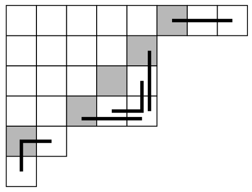
Figure 1. We associate each possible location for a ribbon tile of fixed length $k$ with a cell (shaded) which is above the tile’s lower end and to the left of its upper end. The resulting sequence of cells moves up and to the right at each step, implying that the number of locations is less than $\sqrt{2n}$. Here $k=3$.

Clearly the number of consistent tilings is an upper bound on $\left|\chi_{\lambda}(\pi)\right|$. Now, we claim that for any fixed $k$, the number of possible locations for a ribbon tile of length $k$ on the boundary of a Young diagram $\lambda$ of size $n$ is less than $\sqrt{2n}$. To see this, associate each one with the cell of $\lambda$ which is directly above the tile’s lower end, and directly to the left of its upper end, as shown in Figure 1. A little thought reveals that the resulting sequence of cells has the property that each one is above and to the right of the previous one. Therefore, if there are $\ell$ locations, we have

$$n\geq\sum_{i=1}^{\ell}i>\ell^{2}/2\enspace.$$

and so $\ell<\sqrt{2n}$. It follows that the number of ways to remove the ribbon tiles corresponding to the $c(\pi)$ nontrivial cycles is less than

$$(2n)^{c(\pi)/2}\enspace.$$

Moreover, after these ribbon tiles are removed, the number of consistent tilings of the remaining Young diagram is simply the dimension of the corresponding irrep of $S_{n-s(\pi)}$, which is less than $\sqrt{|S_{n-s(\pi)}|}=\sqrt{(n-s(\pi))!}$. Therefore, if $\lambda$ is typical we have

$$\left|\frac{\chi_{\lambda}(\pi)}{d_{\lambda}}\right| <\frac{(2n)^{c(\pi)/2}\sqrt{(n-s(\pi))!}}{e^{-\sqrt{n}\log n}\sqrt{n!}}$$

$$<2\cdot e^{\sqrt{n}\log n}\,2^{c(\pi)/2}\,e^{s(\pi)/2}\,n^{(c(\pi)-s(\pi))/2}$$

$$\leq 2\cdot e^{\sqrt{n}\log n}\,(\sqrt{2}e)^{t(\pi)}\,n^{-t(\pi)/2}\enspace.$$

Here we used the bound $(n-s)!/n!<4\cdot n^{-s}e^{s}$, implied by Stirling’s approximation, and the facts that $c(\pi)\leq t(\pi)$, $s(\pi)\leq 2t(\pi)$, and $t(\pi)=s(\pi)-c(\pi)$. Finally, if $t(\pi)>\sqrt{n}\log n$, the term $e^{\sqrt{n}\log n}$ can be absorbed into $A^{t(\pi)}$, and Lemma holds for any $A>\sqrt{2}e^{2}$. ∎

Lemma 7 (Rattan and Śniady [RŚ06]).

For every $D>0$ there exists a constant $A^{\prime}$ with the following property. If $\lambda$ is a Young diagram with $n$ boxes which has at most $D\sqrt{n}$ rows and columns and $\pi\in S_{n}$ is a permutation then

(22) $$\left|\frac{\chi_{\lambda}(\pi)}{d_{\lambda}}\right|<\left(\frac{A^{\prime}\max(1,t(\pi)^{2}/n)}{\sqrt{n}}\right)^{t(\pi)}.$$

Lemma 8.

All typical irreps $\lambda$ are $O(1)$-smooth.

Proof.

If $\lambda$ is typical, then Lemma 6 implies

$$\sum_{\begin{subarray}{c}\pi\in S_{n}\\ t(\pi)>\sqrt{n}\log n\end{subarray}}\left|\frac{\chi_{\lambda}(\pi)}{d_{\lambda}}\right|^{4}\leq\sum_{\pi\in S_{n}}(A^{t(\pi)}n^{-t(\pi)/2})^{4}=\sum_{\pi\in S_{n}}z^{t(\pi)}$$

for $z=A^{4}/n^{2}$. Since each $\pi\in S_{n}$ appears exactly once in the product

$$\big{[}1+(12)\big{]}\big{[}1+(13)+(23)\big{]}\cdots\big{[}1+(1n)+\cdots+(n-1,n)\big{]}$$

where $(i,j)$ denotes the transposition interchanging $i$ and $j$, and since each product of the summands provides a factorization of $\pi$ into a minimal number of transpositions, we have

$$\sum_{\pi\in S_{n}}z^{t(\pi)}=(1+z)(1+2z)\cdots(1+(n-1)z)<\\ e^{z}e^{2z}\cdots e^{(n-1)z}<e^{zn^{2}/2}=e^{A^{4}/2}$$

therefore

(23) $$\sum_{\begin{subarray}{c}\pi\in S_{n}\\ t(\pi)>\sqrt{n}\log n\end{subarray}}\left|\frac{\chi_{\lambda}(\pi)}{d_{\lambda}}\right|^{4}<e^{A^{4}/2}\enspace.$$

Very similar but slightly more involved reasoning can be applied to the estimate from Lemma 7 (for details we refer to [RŚ06]) which shows that there exist constants $E>0$ and $E^{\prime}$ (which depend only on $D$) with a property that if a Young diagram $\lambda$ with $n$ boxes has at most $D\sqrt{n}$ boxes in each row and column then

(24) $$\sum_{\begin{subarray}{c}\pi\in S_{n},\\ t(\pi)\leq En^{4/7}\end{subarray}}\left|\frac{\chi_{\lambda}(\pi)}{d_{\lambda}}\right|^{4}\leq E^{\prime}\enspace.$$

The domains of the summations in the inequalities (23) and (24) cover the whole group $S_{n}$ for sufficiently large $n$ which finishes the proof. ∎

Lemma 9.

There are constants $c^{\prime}>0$ and $n_{0}$ such that for all pairs of typical irreps $\lambda$ and $\mu$, if $\tau$ is chosen according to the natural distribution ${{\mathcal{P}}_{\lambda\otimes\mu}(\tau)}$, then $\tau$ is typical with probability at least $1-e^{-c^{\prime}\sqrt{n}}$ if $n>n_{0}$.

Proof.

Let $X$ be the set of atypical representations, and let $\rho=\lambda\otimes\mu$. Then applying Lemma 1 and Lemma 5, using Cauchy-Schwartz as in the proof of Lemma 2, and finally applying Lemma 8 gives

$${\mathcal{P}}_{\lambda\otimes\rho}(X) \leq\sqrt{{\mathcal{P}}_{\rm planch}(X)}\sqrt{\sum_{g\in G}\left|\frac{\chi_{\lambda}(g)}{d_{\lambda}}\right|^{2}\left|\frac{\chi_{\mu}(g)}{d_{\mu}}\right|^{2}}$$

$$\leq e^{-(c/2)\sqrt{n}}\sqrt[4]{\sum_{g\in G}\left|\frac{\chi_{\lambda}(g)}{d_{\lambda}}\right|^{4}\sum_{g\in G}\left|\frac{\chi_{\mu}(g)}{d_{\mu}}\right|^{4}}$$

$$\leq e^{-(c/2)\sqrt{n}}\,O(1)$$

which completes the proof for any $c^{\prime}<c/2$. ∎

7. Proof of the main result

We are now in a position to present our main result.

Theorem 10.

Let $\hat{c},c,c^{\prime}$ be the constants defined above. Then for any constants $a,b$ such that $a+b<\min(\hat{c}/2,c,c^{\prime})$, no sieve algorithm which combines less than $e^{a\sqrt{n}}$ coset states can solve Graph Isomorphism with success probability greater than $e^{-b\sqrt{n}}$.

Proof.

We first consider the behavior of a sieve algorithm $A$ in the case where the hidden subgroup $H\subset S_{n}\wr\mathbb{Z}_{2}$ is trivial. For convenience, let us say that a representation $\sigma_{\{\lambda,\mu\}}$ of $S_{n}\wr\mathbb{Z}_{2}$ is typical if both $\lambda$ and $\mu$ are. We will establish that with overwhelming probability, all the irrep labels observed by $A$ are both typical and inhomogeneous.

Let $\ell$ be the number of coset states initially generated by the algorithm. We begin by showing that with high probability, the irrep labels on the $\ell$ leaves, i.e., those resulting from weak Fourier sampling these coset states, are all both typical and homogeneous. If $H$ is trivial, then these irrep labels are Plancherel-distributed; by (13) the probability that a given one fails to be typical is at most twice the probability that a Plancherel-distributed irrep of $S_{n}$ fails to be, which by Lemma 5 is at most $e^{-c\sqrt{n}}$. Moreover, by (14) the probability that the label of a given leaf is homogeneous is the probability that we observe the same irrep of $S_{n}$ twice in two independent samples of the Plancherel distribution, which using Theorem 3 is

$$\sum_{\lambda}\left(\frac{d_{\lambda}^{2}}{n!}\right)^{\!2}<\max_{\lambda}\frac{d_{\lambda}^{2}}{n!}\leq e^{-\hat{c}\sqrt{n}}\enspace.$$

Thus the combined probability that any of the $\ell$ leaves have a label which is not both typical and inhomogeneous is at most

(25) $$\ell\left(2e^{-c\sqrt{n}}+e^{-\hat{c}\sqrt{n}}\right)\enspace.$$

Now, assume inductively that all the irreps observed by the algorithm before the $i$th combine-and-measure step are typical and inhomogeneous, and that the $i$th step combines states with two such labels $\sigma_{\{\lambda,\lambda^{\prime}\}}$ and $\sigma_{\{\mu,\mu^{\prime}\}}$. By (16), the probability this results in a homogeneous irrep is bounded by the probability ${\mathcal{P}}^{\rm coll}$ of a collision between a pair of natural distributions in $S_{n}$. Then Theorem 3 and Lemmas 2 and 8 and imply that this probability is bounded by

$${\mathcal{P}}^{\rm coll}\leq e^{-(\hat{c}/2)\sqrt{n}}\,O(1)\enspace.$$

In addition, Lemma 9 implies that the the probability the observed irrep fails to be typical is at most $e^{-c^{\prime}\sqrt{n}}$. Since each combine-and-measure step reduces the number of states by one, there are less than $\ell$ such steps; taking a union bound over all of them, the probability that any of the observed irreps fail to be both homogeneous and typical is

(26) $$\ell\left(e^{-(\hat{c}/2)\sqrt{n}}\,O(1)+e^{-c^{\prime}\sqrt{n}}\right)\enspace.$$

Let us call a transcript inhomogeneous if all of its irrep labels are. Combining (25) and (26) and setting $\ell<e^{a\sqrt{n}}$, we see that, for $n$ sufficiently large, $A$’s transcript is inhomogeneous with probability greater than $1-e^{-b\sqrt{n}}$ for any $b<\min(\hat{c}/2,c,c^{\prime})-a$.

Now consider $A$’s behavior in the case of a nontrivial hidden subgroup $H=\{1,m\}$. Inductively applying Equation (12) shows that the probability of observing any inhomogeneous transcript is exactly the same as it would have been if $H$ were trivial. Thus the total variation distance between the distribution of transcripts generated by $A$ in these two cases is less than $e^{-b\sqrt{n}}$, and the theorem is proved. ∎

References

- [AJL06] Dorit Aharonov, Vaughan Jones, and Zeph Landau. A polynomial quantum algorithm for approximating the Jones polynomial. Proc. 38th Symposium on Theory of Computing, 427–436, 2006.
- [AMR06] Gorjan Alagić, Cristopher Moore, and Alexander Russell. Quantum algorithms for Simon’s problem over general groups. Proc. 18th Symposium on Discrete Algorithms (2007).
- [AD95] David Aldous and Persi Diaconis. Hammersley’s interacting particle process and longest increasing subsequences. Probab. Theory Relat. Fields 103 (1995), 199–213.
- [Bab80] László Babai. On the complexity of canonical labeling of strongly regular graphs. SIAM J. Computing, 9(1):212–216, 1980.
- [Bab83] László Babai and Eugene M. Luks. Canonical labeling of graphs. Proc. 15th Symposium on Theory of Computing, 171–183.
- [BCvD05] David Bacon, Andrew Childs, and Wim van Dam. From optimal measurement to efficient quantum algorithms for the hidden subgroup problem over semidirect product groups. Proc. 46th Symposium on Foundations of Computer Science, 469–478, 2005.
- [BCvD06] David Bacon, Andrew Childs, and Wim van Dam. Optimal measurements for the dihedral hidden subgroup problem. Chicago Journal of Theoretical Computer Science, 2006.
- [Bia98] Philippe Biane. Representations of symmetric groups and free probability. Advances in Mathematics, 138(1):126–181, 1998.
- [FIM+03] Katalin Friedl, Gábor Ivanyos, Frédéric Magniez, Miklos Santha, and Pranab Sen. Hidden translation and orbit coset in quantum computing. Proc. 35th Symposium on Theory of Computing, 1–9, 2003.
- [Ful97] William Fulton. Young Tableaux: with Applications to Representation Theory and Geometry, volume 35 of Student Texts. London Mathematical Society, 1997.
- [GSVV01] Michelangelo Grigni, Leonard Schulman, Monica Vazirani, and Umesh Vazirani. Quantum mechanical algorithms for the nonabelian hidden subgroup problem. Proc. 33rd Symposium on Theory of Computing, 68–74, 2001.
- [Hal02] Sean Hallgren. Polynomial-time quantum algorithms for Pell’s equation and the principal ideal problem. Proc. 34th Symposium on Theory of Computing, 653–658.
- [Hal05] Sean Hallgren. Fast quantum algorithms for computing the unit group and class group of a number field. Proc. 37th Symposium on Theory of Computing, 468–474, 2005.
- [HMR+06] Sean Hallgren, Cristopher Moore, Martin Rötteler, Alexander Russell, and Pranab Sen. Limitations of quantum coset states for graph isomorphism. Proc. 38th Symposium on Theory of Computing, 604–617, 2006.
- [HRTS00] Sean Hallgren, Alexander Russell, and Amnon Ta-Shma. Normal subgroup reconstruction and quantum computation using group representations. Proc. 32nd Symposium on Theory of Computing, 627–635, 2000.
- [JK81] Gordon James and Adalbert Kerber. The representation theory of the symmetric group, volume 16 of Encyclopedia of mathematics and its applications. Addison–Wesley, 1981.
- [Ker03] S. V. Kerov. Asymptotic representation theory of the symmetric group and its applications in analysis, volume 219 of Translations of Mathematical Monographs. American Mathematical Society, 2003. Translated by N. V. Tsilevich.
- [Kup05] Greg Kuperberg. A subexponential-time quantum algorithm for the dihedral hidden subgroup. SIAM J. Computing 35(1): 170–188, 2005.
- [MR05a] Cristopher Moore and Alexander Russell. Explicit multiregister measurements for hidden subgroup problems; or, Fourier sampling strikes back. Preprint, quant-ph/0504067 (2005).
- [MR05b] Cristopher Moore and Alexander Russell. The symmetric group defies strong Fourier sampling: part II. Preprint, quant-ph/0501066 (2005).
- [MR06] Cristopher Moore and Alexander Russell. On the impossibility of a quantum sieve algorithm for Graph Isomorphism. Preprint, quant-ph/0609138 (2006).
- [MRS04] Cristopher Moore, Alexander Russell, and Leonard Schulman. The power of basis selection in fourier sampling: hidden subgroup problems in affine groups. Proc. 15th Symposium on Discrete Algorithms, 1113–1122, 2004.
- [MRS05] Cristopher Moore, Alexander Russell, and Leonard Schulman. The symmetric group defies Fourier sampling. Proc. 46th Symposium on Foundations of Computer Science, 479–488, 2005.
- [RŚ06] Amarpreet Rattan and Piotr Śniady. Upper bound on the characters of the symmetric groups for balanced Young diagrams and a generalized Frobenius formula. Preprint, math.RT/0610540 (2006).
- [Reg02] Oded Regev. Quantum computation and lattice problems. Proc. 43rd Symposium on Foundations of Computer Science, 520–529, 2002.
- [Ser77] Jean-Pierre Serre. Linear Representations of Finite Groups. Number 42 in Graduate Texts in Mathematics. Springer-Verlag, 1977.
- [Sho94] Peter W. Shor. Algorithms for quantum computation: discrete logarithms and factoring. Proc. 35th Symposium on Foundations of Computer Science, 124–134, 1994.
- [Sim94] D. R. Simon. On the power of quantum computation. Proc. 35th Symposium on Foundations of Computer Science, 116–123, 1994.
- [Spi96] Daniel A. Spielman. Faster isomorphism testing of strongly regular graphs. Proc. 28th Symposium on Theory of Computing, 576–584, 1996.
- [VK85] A. M. Vershik and S. V. Kerov. Asymptotic behavior of the maximum and generic dimensions of irreducible representations of the symmetric group. Funk. Anal. i Prolizhen, 19(1):25–36, 1985. English translation, Funct. Anal. Appl. 19(1):21–31, 1989.