Singularity of Berry Connections Inhibits the Accuracy of Adiabatic Approximation

Abstract

Adiabatic approximation for quantum evolution is investigated quantitatively with addressing its dependence on the Berry connections. We find that, in the adiabatic limit, the adiabatic fidelity may uniformly converge to unit or diverge manifesting the breakdown of adiabatic approximation, depending on the type of the singularity of the Berry connections as the functions of slowly-varying parameter $R$. When the Berry connections have a singularity of $1/R^{\sigma}$ type with $\sigma<1$, the adiabatic fidelity converges to unit in a power-law; whereas when the singularity index $\sigma$ is larger than one, adiabatic approximation breaks down. Two-level models are used to substantiate our theory.

The adiabatic theorem, as a fundamental theorem in quantum mechanics, plays a crucial role in our understand and manipulation of microscopic worldrev1 . Recent years witness its growing importance in the context of quantum control, for example, concerning adiabatic transportation of the newly formed matter — Bose-Einstein condensateliu1 , as well as for adiabatic quantum computationfu .

Despite the existence of an extensive literatureaddadd on proofs of estimates needed to justify the adiabatic approximation, doubts have been raised about its validity leading to confusion about the precise conditions needed to use it ref1 ; ref2 . In the present paper, we point out that the above confusions can be avoided with formulating the quantum adiabatic approximation within parameter domain rather than time domain. Within this formulation, we address the fidelity of the adiabatic approximation quantitatively (up to the prefactors of power-law or exponential forms). In particular, we find that in the adiabatic limit, the behavior of adiabatic fidelity depends on the singularity of the Berry connections. That is, the Berry connections of the system determine how good the adiabatic approximation is. As we know, in adiabatic quantum search algorithms, the upper bound of adiabatic fidelity (measure of distance between exactly solution and adiabatic approximation) is essential to the search time fidelity ; wys .

The system we consider is a Hamiltonian containing slowly-varying dimensionless parameters $\mathbf{R}(t)$ belongs to a given regime $[\mathbf{R}_{0},\mathbf{R}_{1}]$, saying, $H(\mathbf{R}(t))$. Initially we have a state, for example, the ground state $|E_{0}(\mathbf{R}(t_{0}))\rangle$ with energy $E_{0}(\mathbf{R}(t_{0}))$. The wave function $|\Psi(t)\rangle$ fulfills the usual Schrödinger equation, i.e., $i\frac{d\Psi}{dt}=H(\mathbf{R}(t))\Psi(t)$, with $\hbar=1$. The above problem has a well-known adiabatic approximate solution ,

$$|\Psi_{ad}>=e^{-i\int^{t}E_{0}dt}e^{i\gamma_{0}}|E_{0}(\mathbf{R}(t))>.$$ (1)

with $\gamma_{0}=i\int^{t}dt<E_{0}|\dot{E}_{0}>,$ the geometric phase term berry ; liu . The above equation is the explicit formulation of the adiabatic theorem stating that the initial nondegenerate ground state will remain to be the instantaneous ground state and evolve only in its phase, given by the time integral of the eigenenergy (known as the dynamical phase) and a quantity independent of the time duration (known as the geometric phase).

The problems is, how close the above adiabatic approximate solution to the real solution $|\Psi(t)\rangle$. To clarify the above question and formulate it quantitatively, we introduce two physical quantities, namely, adiabatic parameter and adiabatic fidelity, respectively.

The dimensionless adiabatic parameter is defined as the ratio between the change rate of the external parameters and the internal characteristic time scales of the quantum system (i.e., the Rabi frequency $|E_{m}-E_{n}|$), used to measure how slow the external parameter changes with respect to time,

$$\epsilon=max\frac{|\mathbf{\dot{R}}|}{|E_{n}(\mathbf{R})-E_{m}(\mathbf{R})|},m\neq n.$$ (2)

$\epsilon\to 0$ corresponds to adiabatic limit.

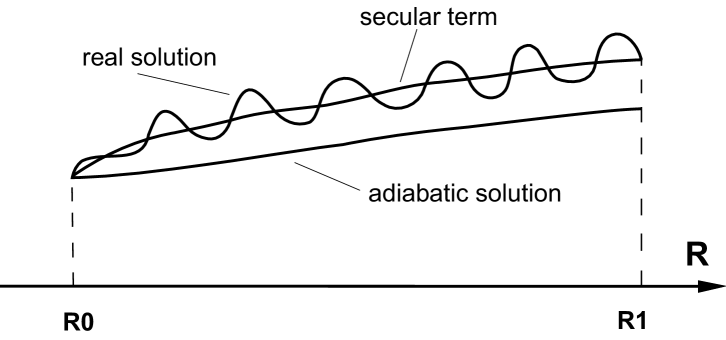
Figure 1: Schematic illustration of the quantum adiabatic evolution formulated in parameter condition, see text for detailed description.

Adiabatic fidelity is introduced to measure how close the adiabatic solution to real one, $F_{ad}=|\langle\Psi(t)|\Psi_{ad}\rangle|^{2}$. The convergence of the the adiabatic fidelity to unit uniformly in the range $\mathbf{R}\in[\mathbf{R}_{0},\mathbf{R}_{1}]$ in the adiabatic limit ($\epsilon\to 0$), indicates the validity of the adiabatic approximation. Evaluating fidelity function will give an estimation on how good the adiabatic approximation is.

In Fig.1 we schematically illustrate the physical process we describe above. Our main result is that, the distance between the adiabatic solution and real one consists two parts: the fast oscillation term and the secular term. The time scale of the oscillation is the Rabi period, its amplitude is proportional to the square of the adiabatic parameter. The amplitude of the secular term is exponential small ($\sim\exp{-1/\epsilon}$) suppose that the Berry connections of the system are regular, and turn to be power-law ($\sim\epsilon^{x},x<2$) if the Berry connections have singularity or the external parameters vary in time nonlinearly.

We start our statement with writing the wavefunction as a superposition of the instantaneous eigenstates, $|\Psi(t)\rangle=\sum_{n}C_{n}(t)e^{-i\int^{t}dt(E_{n}-i\langle E_{n}(R)|\dot{E}_{n}(R)\rangle)}|E_{n}(\mathbf{R}(t))\rangle$, and suppose initial state is the ground state, i.e., $C_{0}(t=0)=1,C_{n}(t=0)=0,(n\neq 0)$. Then the adiabatic approximate solution takes form of Eq.(1) and the adiabatic fidelity $F_{ad}=|\langle\Psi(t)|\Psi_{ad}\rangle|^{2}=|C_{0}|^{2}\sim 1-|\Delta C_{n}|^{2},(n\neq 0)$ . To evaluate the adiabatic fidelity we need quantitatively evaluate the change of the coefficients $C_{n}$ with respect to time.

Substituting the above solution into Schrödinger equation, we have following differential equation for the coefficients,

$$\frac{d}{dt}C_{n}=i\sum_{m\neq n}e^{i\int^{t}((E_{n}-\mathbf{\alpha}_{nn}\mathbf{\dot{R}})-(E_{m}-\mathbf{\alpha}_{mm}\mathbf{\dot{R}}))dt}\mathbf{\alpha}_{nm}(\mathbf{R})\frac{d\mathbf{R}}{dt}C_{m}.$$ (3)

where $\alpha_{nm}(\mathbf{R})$ is the Berry connection. Both off-diagonal and diagonal Berry connections have clear physical meaning and important applicationsoffdia . We first suppose these Berry connections and the gradient of instantaneous eigenenergy are not singular (NS) as the functions of the external parameters, i.e.,

$$\mathbf{\alpha}_{nm}(\mathbf{R})=\langle E_{n}|i\nabla_{\mathbf{R}}|E_{m}\rangle;\mathbf{\beta}_{n}(\mathbf{R})=\nabla_{\mathbf{R}}E_{n}(\mathbf{R}),\mathit{NS}.$$ (4)

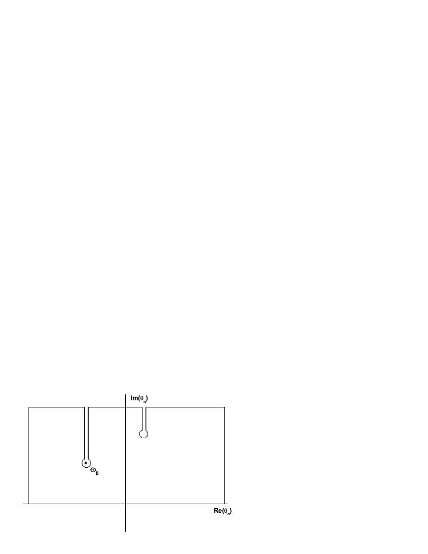
Figure 2: The integral path and the singular points in the complex plane.

Under the above condition and in the adiabatic limit, to estimate the distance between the adiabatic solution and the real one, we need quantitatively evaluate the change of the coefficients $C_{n}$ with respect to time. The right-hand of Eq.(3) contains unknown $C_{m}$, to the first order of approximation, we take $C_{0}=1$ and $C_{m}=0,m\neq 0$ in the right-hand of Eq.(3). Then, Eq.(3) shows that, the change consists two parts: the fast oscillation term and the secular term. The time scale of the oscillation is the Rabi period, its amplitude is proportional to the adiabatic parameter suppose that the Berry connections are regular with limitation. Whereas the secular term maybe is exponential small of form $e^{-\frac{1}{\epsilon}}$ or power-law depending on the Berry connections in following.

Let us denote $\theta_{n}=\int^{t}(E_{n}-E_{0})dt$, and then the upper bound of the increment on the coefficients ($n\neq 0$) can be evaluated as follows

$$\Delta C_{n} \sim \int_{\theta_{n}(\mathbf{R}_{0})}^{\theta_{n}(\mathbf{R}_{1})}\frac{e^{i\theta_{n}}}{E_{n}-E_{0}}\mathbf{\alpha}_{n0}\dot{\mathbf{R}}d\theta_{n}$$ (5)

$$= \int_{\mathbf{-\infty}}^{\mathbf{\infty}}...d\theta_{n}\mathbf{-}\left(\int_{\mathbf{-\infty}}^{\theta_{n}(\mathbf{R}_{0})}\mathbf{+}\int_{\theta_{n}(\mathbf{R}_{1})}^{\mathbf{\infty}}\right)...d\theta_{n}$$ (6)

where we set that in the right-hand of Eq.(3) the coefficients $C_{m}\sim 0$ for $m\neq 0,$ and $C_{0}\sim 1$ since we want to estimate the upper bound of the adiabatic approximation. For simple and without losing generalization, in following deductions we regards the slowly-varying as a scalar quantity, and assume that $\frac{dR}{dt}\sim\epsilon g(R)$ with function $g(R)$ being regular with limitation.

The main contribution to the first term on the right hand comes from the pole point, $\theta_{n}^{c}=\int^{t_{c}}(E_{n}-E_{0})dt\sim\frac{1}{\epsilon}\int^{R_{c}}(E_{n}-E_{0})/g(R)dR$, determined by the equation $E_{n}(\mathbf{\theta^{c}}_{n})-E_{0}(\mathbf{\theta^{c}}_{n})=0$. Because the non-degeneracy of the system, the solutions of the above pole points are complex with imaginary parts. Let $\omega_{0}$ be the singularity nearest the real axis, i.e., the one with the smallest (positive) imaginary part (see Fig.2). Then, the first term is approximately bounded by $exp(-Im\omega_{0})\sim e^{-\frac{1}{\epsilon}|\int^{|Im(R_{c})|}(E_{n}-E_{0})/g(R)dR|}$, which is just the secular term and is exponential small in adiabatic limitliuliu . The second integral is proportional to $\epsilon$, which gives the estimation on the fast oscillation term.

Now, we consider the situation that Berry connection has singularity in the parameter regime $[\mathbf{R}_{0},\mathbf{R}_{1}]$, e.g., $R=0$, taking the form $\frac{1}{R^{\sigma}}$. We then evaluate the above integral in the neighborhood domain $[-\epsilon,\epsilon]$ of the singular point, other regime is regular and can be treated in the same way as before. Then,

$$|\Delta C_{n}|\sim|\int_{-\epsilon}^{\epsilon}e^{i\int^{t}(E_{n}-E_{0})dt}\mathbf{\alpha}_{n0}(R)dR|\sim\epsilon^{(1-\sigma)}.$$ (7)

The situation is divided into two cases: $\sigma<1$ and $\sigma\geq 1$. For $\sigma<1$, this type of singularity can be removed because the integral is finite. The integral in the neighborhood domain $[-\epsilon,\epsilon]$ of the singularity contributes a quantity of order $\epsilon^{(1-\sigma)}$, We thus expect that the adiabatic fidelity approaches to unit uniformly in the $2(1-\sigma)$ power-law of the adiabatic parameter, i.e.,

$$1-F_{ad}\sim\epsilon^{2(1-\sigma)}.$$ (8)

For the case of $\sigma\geq 1$, the singularity is irremovable and the adiabatic approximation is expected to break down.

The above discussions is readily extended to the case that the slowing-varying parameters change nonlinearly with time, i.e., $R=\epsilon t^{\sigma}$, with $\sigma$ is any positive number. The nonlinear time dependent parameter has many physical origins, for example in molecule spin system the effective field vary in time nonlinearlynonlinear1 . Another field of broad examples is quantum optics, Rabi frequency coupling different levels (i.e., stimulated Raman adiabatic passage) is usually nonlinear dependence on time nonlinear2 . Here we suppose that the Berry connections of quantum system are regular with limitation as the function of the parameter $R$ and the level spacings are of order 1. To apply our theory, we introduce the new parameters $R^{\prime}$ and $\epsilon^{\prime}$ through the expressions $\epsilon^{\prime}=\epsilon^{\frac{1}{\sigma}}$ and $R^{\prime}=\epsilon^{\prime}t$. Then, $R={R^{\prime}}^{\sigma}$. As a function of the new parameter $R^{\prime}$, the singularity of the Berry connections determined by the $\frac{dR}{dR^{\prime}}\sim 1/{R^{\prime}}^{1-\sigma}$. Our discussions are divided into two cases: i) $\sigma>1$ and ii) $\sigma<1$. In the former case, the Berry connections as the functions of the new parameter are regular, so the adiabatic fidelity is determined by the short-term oscillation and is expected to converge to one in a power-law of $\epsilon^{\prime 2}$. Then we have

$$1-F_{ad}\sim\epsilon^{\frac{2}{\sigma}}.$$ (9)

In the latter case, the Berry connections as the functions of the new parameter are singular of type $1/{R^{\prime}}^{1-\sigma}$. Fortunately, this singularity is removable, it gives an upper bound of the adiabatic Fidelity as $\epsilon^{\prime 2\sigma}$, i.e.,

$$1-F_{ad}\sim\epsilon^{2}.$$ (10)

Notice that in this case, the upper bound of the adiabatic fidelity is independence of the nonlinear index $\sigma$ .

In following, we use two-level models to substantiate the above discussions. Our model is denoted by $S^{a}$: a spin-half particle in a rotating magnetic field, its Hamiltonian reads,

$$H^{a}(R(t)) = -\frac{\omega_{0}}{2}(\sin\theta\cos f(R(t))\sigma_{x}+\sin\theta\sin f(R(t))\sigma_{y}$$ (11)

$$+\cos\theta\sigma_{z}),$$

$\omega_{0}$ is defined by the strength of the magnetic field, and $\sigma_{i},$ $(i=x,y,z)$ are Pauli matrices. $f(R)$ is a function of slowly-varying parameter $R.$ The above $2\times 2$ matrix is readily diagonalized for fixed $R$ and we then obtain its instantaneous  eigenenergies $E_{\pm}^{a}=\pm\frac{\omega_{0}}{2}$, and instantaneous eigenvectors,

$$|E_{-}^{a}(R)\rangle=\left(\begin{array}[]{c}e^{-i\frac{f(R)}{2}}\sin\frac{\theta}{2}\\ -e^{i\frac{f(R)}{2}}\cos\frac{\theta}{2}\end{array}\right),|E_{+}^{a}(R)\rangle=\left(\begin{array}[]{c}e^{-i\frac{f(R)}{2}}\cos\frac{\theta}{2}\\ e^{i\frac{f(R)}{2}}\sin\frac{\theta}{2}\end{array}\right)$$ (12)

The Berry connections are derived as follows,

$$\alpha^{c}_{--}=\frac{1}{2}\cos\theta\frac{df}{dR},\;\alpha^{c}_{-+}=\frac{1}{2}\sin\theta\frac{df}{dR}.$$ (13)

Figure 3: Adiabatic fidelity evolves for different type of singularity.

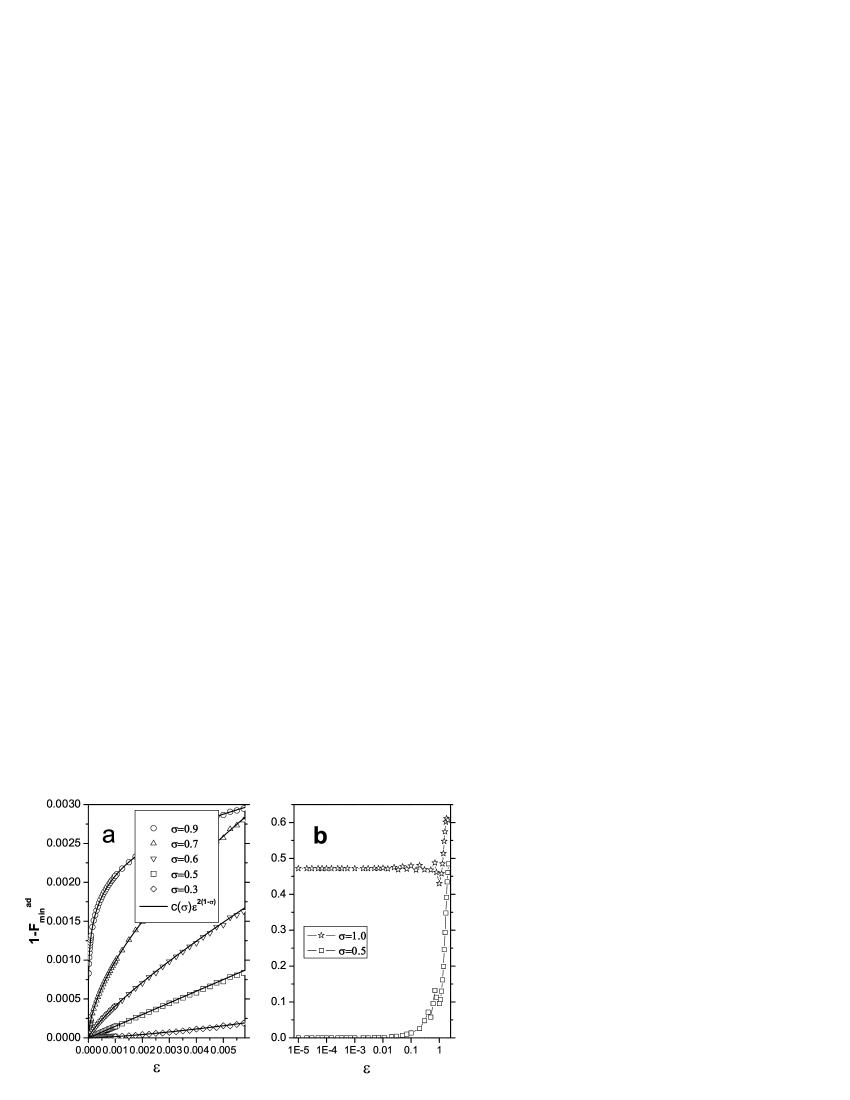
Figure 4: Upper bound of the adiabatic fidelity in system $S^{c}$ for different type of singularity. $F^{ad}_{min}$ is the minimum fidelity in the parameter range $\mathbf{R}\in[-2\pi,2\pi]$

i)We first consider following two cases: $f(R)=\ln|R|$ and $f(R)=|R|^{1-\sigma}$ with $\sigma<1$, respectively. And here the slowly-varying parameter is supposed to linearly change with time, i.e., $R(t)=\omega t$. $\omega$ is the rotating frequency of the magnetic field. Apparently, the Berry connection has singularity of the form $1/R^{\sigma}$ at point $R=0$ . These systems are complicated and analytic solutions are not reachable. We thus make numerical simulations on the adiabatic fidelity by directly solving the Schrödinger equation with the $4^{th}-5^{th}$ Runge-Kutta adaptive step method. Our results are shown in Fig.3 and Fig.4. In the Fig.3, it is clearly shown that, without the singularity (Fig.3a), the distance between the adiabatic solution and real solution is determined by the fast oscillation, therefore gives the upper bound of square adiabatic parameter. With the singularity (Fig.3b), the upper bound is determined by the type of the singularity of the Berry connections as we discuss above. For the situation that the Berry connections have irremovable singularity (i.e., $\sigma=1$, see Fig.4b) the adiabatic fidelity converges to 0.53 rather than one implying the failure of adiabatic approximation. For the case of the removable singulary of the Berry connection($\sigma<1$) the adiabatic fidelity converges to unit in the power-law dependence of the adiabatic parameters as we expect (see Fig.4a).

ii) We then set $f(R)=R$ and $R$ varies in time nonlinearly, i.e., $R=\epsilon sign(t)|t|^{\sigma}$. In this case, we see that (Fig.5), for $\sigma>1$, the adiabatic fidelity converges to unit in a power-law of exponent $2/\sigma$; for $\sigma<1$, it clearly demonstrates that the exponent turns to be two, independence of the nonlinear index $\sigma$. These numerical simulations corroborate our theory.

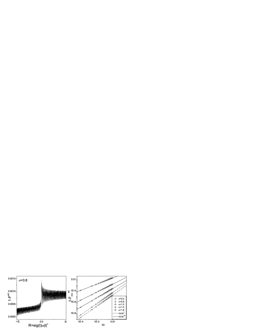
Figure 5: Upper bound of the adiabatic fidelity for different type of the nonlinearly-varying external parameters.

In the above discussion we discuss quantum adiabatic issue under the parameter conditions. We emphasize that the adiabatic problem can only be well formulated in the parameter domain but not in time domain. Therefore, it requires that the Hamiltonian depends on the time only through the slowly-varying parameters (i.e., taking form $H(R(t))$) and, the range of the parameters (i.e., ($R_{0}$,$R_{1}$)) can be reached at certain time (i.e.,$t_{0}$ and $t_{1}$) for any small adiabatic parameter ($\epsilon$) as sketched in Fig.1. Usually, the smaller the adiabatic parameter, the longer the time duration (i.e., $t_{1}-t_{0}$) is needed. In following we address this point with an example raised in ref2 . It is constructed from $S^{a}$ for the case of $f(R)=R,R=\omega t$ through following relation,

$$H^{ce}=-U^{a\dagger}(t)H^{a}(t)U^{a}(t)$$ (14)

with $U^{a}(t)=T\exp(\int_{0}^{t}H^{a}(t^{\prime})dt^{\prime})$ the time evolution operator of system $S^{a}$. Its explicit analytic expression is readily obtained ref2 . After lengthy deduction, we obtain the explicit expression of the Hamiltonian $H^{ce}=\frac{\omega_{0}}{2}\mathbf{L}(t)\cdot\mathbf{\sigma},$ where $\mathbf{L}(t)=(\sin\theta(\omega_{0}^{2}+2\omega\omega_{0}\cos\theta\cos^{2}\varpi t/2+\omega^{2}\cos\varpi t)/\varpi^{2},\frac{\omega\sin\theta}{\varpi}\sin\varpi t,$ $\cos\theta+\frac{2\omega\omega_{0}\sin\theta}{\varpi^{2}}\sin^{2}\theta\sin^{2}\varpi t/2),$ and $\varpi=\sqrt{\omega_{0}^{2}+\omega^{2}+2\omega\omega_{0}\cos\theta}$.

It is easy to verify that $\mathbf{L}(t)$ is a unit vector, i.e, $|\mathbf{L}(t)|=1.$ The eigenvalues and eigenvectors for this system are,

$$E_{\pm}^{ce}=\pm\frac{\omega_{0}}{2},\;\;\left|E_{\pm}^{ce}(\mathbf{L})\right\rangle=\left(\begin{array}[]{c}\sqrt{\frac{1\pm L_{3}}{2}}e^{-i\phi}\\ \mp\sqrt{\frac{1\mp L_{3}}{2}}e^{i\phi}\end{array}\right),$$ (15)

where $\phi=\frac{1}{2}\arctan(L_{2}/L_{1}).$ We then can obtain the Berry connections as follows,

$$\mathbf{\alpha}_{--}^{ce} = (\frac{L_{2}L_{3}}{2(1-L_{3}^{2})},-\frac{L_{1}L_{3}}{2(1-L_{3}^{2})},0),$$

$$\mathbf{\alpha}_{-+}^{ce} = (-\frac{L_{2}}{2\sqrt{1-L_{3}^{2}}},\frac{L_{1}}{2\sqrt{1-L_{3}^{2}}},-\frac{i}{2\sqrt{1-L_{3}^{2}}}).$$ (16)

As $L_{3}<1$, the Berry connections are not singular. For $d|\mathbf{L|}/dt\sim\omega$, the adiabatic parameter of this system is $\epsilon=\omega/\omega_{0}.$

The controversy is that, even though in the adiabatic limit $\epsilon\to 0$, the adiabatic fidelity calculated in the time domain $t\in[-2\pi,2\pi]$ does not diverge to unitref2 . Moreover, with changing the sign of the above Hamiltonian and re-calculating the adiabatic fidelity in the time domain $[-2\pi,2\pi]$, we find that the adiabatic fidelity converges to unit in the adiabatic limit. The above result is rather confused. The reason for the above controversy is that the problem is discussed in time domain rather in parameter domain.

To resolve the above controversy, we check the above system in the parameter domain . First, after transformation (14), the $R=\omega t$ acted as the slowly-varying parameter in $H^{a}(t)$ system no longer should be chosen as the slowly-varying parameter of the new system $H^{ce}$, because the Hamiltonian $H^{ce}$ depends explicitly on the time not only through $R$. Instead, $\mathbf{L}(t)$ can serve as the slowly-varying parameters. However, the range of the parameters keeps the same order of the adiabatic parameter (i.e., $|\mathbf{L_{1}}(t=t_{1})-\mathbf{L_{0}}(t=t_{0})|\sim\omega$) and tends to zero in the adiabatic limit no matter how long the evolution time $t_{1}-t_{0}$ is. This completely counters to our picture schematically plotted in Fig.1. Above analysis indicates that the system $H_{ce}$ can not be well formulated in the parameter domain, it essentially not a system that adiabatic theory can applies to. If one discuss the dynamics of this system in the time domain as shown the above, any strange things can happen.

In summary, we investigate the fidelity for quantum evolution under the parameter domain with addressing the adiabatic approximation quantitatively. Within this framework, we clarify the confusions in applying quantum adiabatic theory, and find that the singularity of Berry connections inhibit the accuracy of the adiabatic approximation. Our estimation on the adiabatic fidelity has important meaning in the practical adiabatic quantum search algorithms .

This work was supported by National Natural Science Foundation of China (No.10474008,10604009), Science and Technology fund of CAEP, the National Fundamental Research Programme of China under Grant No. 2005CB3724503, the National High Technology Research and Development Program of China (863 Program) international cooperation program under Grant No.2004AA1Z1220.

References

- (1) P. Ehrenfest, Ann. Phys. (Berlin) 51, 327 (1916); M. Born and V. Fock, Z. Phys. 51, 165 (1928); L. D. Landau, Zeitschrift 2, 46 (1932); C. Zener, Proc. R. Soc. A 137, 696 (1932); J. Schwinger, Phys. Rev. 51, 648 (1937); T. Kato, J. Phys. Soc. Jpn. 5, 435 (1950); M. Gell-Mann and F. Low, Phys. Rev. 84, 350 (1951); M. V. Berry, Proc. R. Soc. A 392, 45 (1984); E. Farhi et al., Science 292, 472 (2001).
- (2) J. Liu, B. Wu, and Q. Niu, Phys. Rev. Lett. 90, 170404 (2003); M. H. Anderson, et. al. Science 269, 198 (1995); K. B. Davis et. al., Phys. Rev. Lett. 75, 3969 (1995); C. C. Bradley et. al., ibid. 75, 1687(1995).
- (3) M.A. Nielsen and I.L. Chuang, Quantum Computation and Quantum Information (Cambridge University Press, Cambridge, 2000); A.M.Childs, et al., Phys. Rev. A 65, 012322 (2002); Li-Bin Fu, Phys. Rev. Lett. 92, 130404 (2004); M. S. Sarandy and D. A. Lidar, Phys. Rev. Lett. 95, 250503 (2005)
- (4) S.Jansen, M.B. Ruskai, R. Seiler, arXiv:quant-ph/060317 (2006) and references therein; B. ReiChardt, Proc. 36:th STOC, p.502(2004); V. Jaksic, J. Math. Phys. 43, 2807 (1993); A.Martinez, J. Math. Phys. 35, 3889 (1994).
- (5) K. Marzlin and B.C. Sanders, Phys. Rev. Lett. 93, 160408 (2004).
- (6) D.M. Tong, K. Singh, L.C. Kwek, and C.H. Oh, Phys. Rev. Lett. 95, 110407 (2005).
- (7) Jérémie Roland, Nicolas J. Cerf, Phys. Rev. A 65, 042308 (2002).
- (8) Yu Shi and Yong-Shi Wu, Phys. Rev. A 69, 024301 (2004).
- (9) M. V. Berry, Proc. R. Soc. London A 392, 45–57 (1984); Geometric Phase in Physics, edited by A. Shapere and F. Wilczek (World Scientific, Singapore, 1989).
- (10) Recent progress on Berry phase refer to, Jie Liu, Bambi Hu, and Baowen Li Phys. Rev. Lett. 81, 1749 (1998); B. Wu, J. Liu, and Q, Niu, Phys. Rev. Lett. 94, 140402 (2005) and references therein.
- (11) Nicola Manini and F. Pistolesi Phys. Rev. Lett. 85, 3067 (2000); Y. Hasegawa, R. Loidl, M. Baron, G. Badurek, and H. Rauch Phys. Rev. Lett. 87, 070401 (2001); Stefan Filipp and Erik Sjöqvist Phys. Rev. Lett. 90, 050403 (2003); Hon Man Wong, Kai Ming Cheng, and M.-C. Chu Phys. Rev. Lett. 94, 070406 (2005).
- (12) The celeberated Landau-Zener model is of this exponential type tunnelling probability, see Jie Liu et al Phys. Rev. A 66,023404 (2002) and references therein..
- (13) D. A. Garanin, R. Schilling, Phys. Rev. B. 66, 174438(2002); A.Hanns, et al,Phys. Rev. B. 62, 13880(2000).
- (14) For example see, K. Bergmann, H. Theuer, and B. W. Shore, Rev. Mod. Phys. 70, 1003(1998)..