Detecting Hidden Differences via Permutation Symmetries

Abstract

We present a method for describing and characterizing the state of $N$ particles that may be distinguishable in principle but not in practice due to experimental limitations. The technique relies upon a careful treatment of the exchange symmetry of the state among experimentally accessible and experimentally inaccessible degrees of freedom. The approach we present allows a new formalisation of the notion of indistinguishability and can be implemented easily using currently available experimental techniques. Our work is of direct relevance to current experiments in quantum optics like Mitchell et al. (2004); Eisenberg et al. (2005); Liu et al. (2006), for which we provide a specific implementation.

The predominant paradigm of quantum information science is the qubit, a quantum two-level system. This useful notion has allowed many important concepts to be abstracted away from particular physical implementations, revealing an underlying structure in the way that information is manipulated and measured in quantum mechanics. Qubits are usually realised in some degree of freedom of a physical system. In many systems such as trapped ions and nuclear spins, the physical particles are inherently separated and the quantum statistical nature of the particles, be they bosons or fermions, can safely be neglected. In other systems including quantum optics, degenerage atomic gases, optically trapped atoms, and quasi-particles such as polaritons, the quantum statistics of the particles can often play a role in the system’s behaviour. Sometimes the quantum statistical behaviour can be very useful, as in the Hong-Ou-MandelHong et al. (1987) effect in quantum optical systems which is often used to post-selectively implement interactions between photonsKnill et al. (2001).

If a quantum information experiment is set up so that each particle is uniquely different in some observable degree of freedom – photons occupying different arms of an interferometer, say, or ions in different locations in a trap – then the quantum statistical properties of the particles generally do not play a role. Characterization of the quantum state of such systems proceeds according to the well-known procedures of quantum state tomographyNielsen and Chuang (2000). The influence of external, unobserved degrees of freedom can be accounted for in this characterization and results in a density matrix displaying less-than-perfect coherence.

Recently, there have been several proposals and experiments involving multiple photons occupying a single spatio-temporal mode and two polarization modesMitchell et al. (2004); Eisenberg et al. (2005); Bogdanov et al. (2004a). Such systems do not fit into the qubit paradigm and quantum statistics plays an integral part in their behaviour. The states of these systems are of enormous interest because they have been shown to exhibit phase superresolution in interferometryMitchell et al. (2004); Boto et al. (2000), to be capable of beating the diffraction limit in lithography Boto et al. (2000); Agarwal et al. (2007); D’Angelo et al. (2001), and to open up new avenues in quantum imagingBennink et al. (2004); Sanders (1989). They have also been proposed as a convenient qutrit useful in certain quantum cryptography and quantum information applicationsBogdanov et al. (2004a); Langford et al. (2004). While, to date, photon systems are the only ones where such states can be created, recent developments in optical latticesFölling et al. (2007) and elsewhere promise to open up similar opportunities in other physical systems in the near future.

Because these states involve multiple occupancy of a single mode, the quantum statistical nature of the particles is crucial to understanding their behaviour. Usually in considering such states the formalism of creation and annihilation operators on the field mode is used. For example, the N00N state $\ket{N,0:0,N}$Boto et al. (2000) can be written as

$$\frac{1}{\sqrt{2(N+1)!}}\left({a_{1}^{\dagger}}^{N}+{a_{2}^{\dagger}}^{N}\right)\ket{0},$$ (1)

where the subscript indexes the distinct modes. When such states are created experimentally, a central task is to reconstruct a faithful characterization of the state from measurement statistics.

Ideally one would prefer to assume nothing about the source of the quantum states, treating it as a ‘black box’, and assume only that one has a set of measurements that one is able to accurately perform on a particular degree of freedom such as polarization. The reconstruction of the state from the measurements is called quantum state tomography and it has been an essential tool in quantum state engineering, quantum information science and quantum computingNielsen and Chuang (2000). If the source produces an indefinite number of photons then continuous variable homodyne tomography methods can be extended to these statesRaymer et al. (2000). If the number of photons is known, though, it is simpler to extend the quantum state tomography techniques developed for qubits to systems of multiply occupied modes, as was done for example by Bogdanov et alBogdanov et al. (2004b).

In their procedure one creates a basis of states from creation operators for a single spatio-temporal mode and the polarization modes that the state can occupy. For the two-photon case that they studied their basis states were $\left\{a_{H}^{\dagger}a_{H}^{\dagger},a_{H}^{\dagger}a_{V}^{\dagger},a_{V}^{\dagger}a_{V}^{\dagger}\right\}$, all taken to act on the vacuum.

There is a subtle assumption in writing the states this way that runs counter to the purpose of quantum state tomography. The notation for the states assumes that the raising operators act on the same spatio-temporal mode, but this is not something that can be experimentally verified from the polarization measurements performed in the tomography. Indeed since the experiment in Bogdanov et al. (2004b) involved combining different spontaneous parametric downconversion sources into a single spatial mode there is every reason to think that the different phase-matching conditions in the two downconversion crystals would result in the raising operators for each source acting on a somewhat different frequency-time mode.

If the two raising operators do indeed act on different spatio-temporal modes then there can be a direct impact on polarization measurements since the amplitudes for different polarizations will carry the bosonic enhancement factors that one obtains by multiplying raising operators on the same mode. In principle one could attempt to fully characterize the spatial and temporal degrees of freedom to obtain the correct raising operator for each photon. Such a full characterization is technically very difficult, if not impossible. Moreover, full information about the spatio-temporal modes is likely not even desireable when it is ultimately polarization that is the degree of freedom of interest.

What one would like is a ‘black box’ tomography technique for reconstructing the state in terms of polarization measurements only. The resulting description of the state ought to somehow include the influence of all unobserved degrees of freedom on polarization measurements. It ought also to correctly predict the outcome of any polarization measurement one wishes to perform so as to be considered ‘tomographically complete’. This paper develops and analyzes exactly such a technique.

To our knowledge the problem of charactizing the state of multiply occupied modes has only arisen experimentally in photonic polarization systems. While we will concentrate on this specific realization, our method is completely general and can be applied to any of the aforementioned physical systems in which quantum statistics play a role, either bosonic or fermionic. In order to have the discussion that follows reflect this generality we will define some technical language. We will call the information-carrying degree of freedom in such systems the ‘visible’ degree of freedom. In the case of photonic polarization systems such as in Bogdanov et al. (2004b); Mitchell et al. (2004) this is polarization. All other degrees of freedom to which the apparatus is not sensitive we call ‘hidden’. The description of the state that results from our state tomography procedure we label the ‘accessible’ density matrix $\rho_{\text{acc}}$.

While inspired by practical problems encountered in our attempts to characterize quantum states, our approach is interesting in its own right as an exploration of how adding distinguishing information in experimentally inaccessible degrees of freedom affects the quantum statistical properties of states.

The key to our approach is to separate the state explicitly into hidden and visible parts and to examine the constraints placed on the visible degree of freedom by the quantum statistical requirements on the whole state. For photons, the bosonic statistics require that the whole state be invariant under exchange of all particle labels. The exchange symmetry is more easily studied in state notation rather than raising operator notation, so we will use state notation throughout this paper. This can be confusing at first because often in the literature states are written in a way that does not make the exchange symmetry explicit. For example, one might write the polarization state of two photons as $\ket{HV}$, which is not obviously exchange-symmetric as it must be for bosons. In such a description the order of the two labels implies the existence of a degree of freedom other than polarization, say different spatial modes $a$ and $b$. $a$ and $b$ could be, for example, the distinguishable output angles of downconverted photons in spontaneous parametric downconversion. The full bosonic state needs to be symmetric under exchange of both spatial and polarization degrees of freedom, and would be written as $\ket{\psi_{1}}=\left(\ket{HV}\ket{ab}+\ket{VH}\ket{ba}\right)/\sqrt{2}$. Note that exchange of both the spatial and polarization labels leaves the state invariant, but the state has the property that one of the spatial modes, $a$ is always correlated with one polarization $H$ and the other mode $b$ is always correlated with polarization $V$. In cases where the individual photon polarizations can be treated as qubits because $a$ and $b$ are distinguishable paths, this notation is redundant because no use is made of the permutation properties of the whole state. For this reason it is usually preferable to write the state as $\ket{H_{a}V_{b}}$ which denotes the correlation between spatial and polarization modes without making explicit the bosonic exchange symmetry. It should be understood that in all circumstances this way of writing the state is simply a shorthand for $\ket{\psi_{1}}$.

We emphasize this point because we wish to discuss situations where the overall exchange symmetry of the state is important and the notation of $\ket{\psi_{1}}$ becomes very useful. There are situations where the spatial modes in the above example are ‘hidden’, that is to say they are not resolved by the detection apparatus. This might occur if the photons were nearly collinear, but with a small angle between them. A multimode collection system such as a lens focusing onto a photodetector significantly larger than the optical wavelength would have no means of distinguishing these two slightly different spatial modes. More generally, there could also be unresolvable ‘hidden’ time-frequency modes that can become occupied due to uncorrected delays or dispersion. Since the nanosecond-scale resolution of most single-photon detectors is much longer than the femtosecond timescale of pulsed experiments, different time-frequency modes are generally not resolved by detectors. In non-photonic systems there are also myriad reasons why a given degree of freedom might be ‘hidden’ from experimental measurements. When a hidden degree of freedom is different for two particles we sometimes say that the particles are distinguishable in principle but not in practice.

We can express our ignorance about the state of these ‘hidden’ degrees of freedom by tracing over them. This leaves a density matrix observable only in the visible degrees of freedom that we call the accessible density matrix:

$$\rho_{\text{acc}}=\text{Tr}_{\text{hid}}\left[\rho\right]\,.$$ (2)

For example, if in the state $\ket{\psi_{1}}$ the modes $a$ and $b$ cannot be resolved then we trace over them to obtain the accessible density matrix

$$\rho_{\text{acc}} =\text{Tr}_{\text{hid}}\left[\ket{\psi_{1}}\bra{\psi_{1}}\right]$$ (3)

$$={\frac{1}{2}}\ket{HV}\bra{HV}+{\frac{1}{2}}\ket{VH}\bra{VH}\,$$ (4)

This is a mixed state of polarization. If the two photons had occupied the same spatial mode so that the state was $\left(\ket{HV}\ket{aa}+\ket{VH}\ket{aa}\right)/\sqrt{2}$, then tracing over the spatial degree of freedom would have yielded a pure accesible density matrix in polarization $\frac{1}{2}\left(\ket{HV}+\ket{VH}\right)\left(\bra{HV}+\bra{VH}\right)$. Since these two situations yield different density matrices on the polarization degree of freedom they can be distinguished by polarization measurements alone. The particular feature that distinguishes them is the antisymmetric part, expressed as the population of the singlet state $\left(\ket{HV}-\ket{VH}\right)/\sqrt{2}$. The singlet state projection makes up one element of the accessible density matrix. It is a measurable quantity even when the experimental apparatus cannot tell the two photons apart. As we discuss extensively in Adamson et al. (2007), for two photons the presence of an antisymmetric component of the polarization state implies the existence of one or more unobserved degrees of freedom that are different for the two particles and correlated in just the right way to result in the correct bosonic exchange symmetry for the whole state. This shows that differences in the hidden degrees of freedom may be inferred from measurements performed only on the visible degrees of freedom.

The remainder of this paper will examine how the accessible density matrix can be calculated and measured for an arbitrary number of particles and for a visible degree of freedom with an arbitrary, finite number of levels. In the first section we will begin by determining how many elements are contained in a general accessible density matrix as a function of the dimensionality of the visible degree of freedom and the number of particles. This determines both how many linearly independent measurements can be made and how many numbers are needed to calculate all possible expectation values on the visible degrees of freedom. The second section will put the discussion of the first section on a firm group-theoretical footing. In the third section we examine how the theory applies to the case of three photon polarizations. In section 4 we discuss how the accessible density matrix can be measured and work through a specific numerical example with three photons. Finally, in section 5 we discuss what claims can be made about the indistinguishability of the particles from a knowledge of the accessible density matrix.

I The form of the accessible density matrix

In this section we develop the structure of the accessible density matrix and show how many independent measurements can be done on a visible degree of freedom. We will start by assuming a two-level degree of freedom like photon polarization and then extend the result to a $d$-level degree of freedom that could, for example, be the Laguerre-Gauss spatial modeLangford et al. (2004) of photons.

Our approach is to consider the Hilbert space of the photons as a tensor product of a Hilbert space describing the visible degrees of freedom and another describing the hidden degrees of freedom. Consider $N$ photon polarizations. Polarization transformations $e^{i\left(x\sigma_{x}+y\sigma_{y}+z\sigma_{z}\right)}$ (where $\set{\sigma_{x},\sigma_{y},\sigma_{z}}$ are the Pauli matrices) give a realization of the group SU(2). Since SU(2) acts irreducibly on the photon polarization, we can view the photons as spin one-half systems; that is, they transform according to the $j=\frac{1}{2}$ irrep of SU(2). If all systems are distinguishable in practice, so that each photon is in a separate mode that can be experimentally distinguished (different rails of a multi-rail interferometer, say), then the dimension of the accesible space is the full dimension $2^{N}$ and the number of accessible density matrix elements is $2^{2N}$. This is the familiar situation of quantum state tomography as applied to photon polarizationJames et al. (2001), trapped ions and other qubit systems. We would like to know the comparable number of density matrix elements when the photons are not experimentally distinguishable because the degrees of freedom that might distinguish the particles cannot be resolved experimentally. We note that in this case $2^{2N}$ provides an upper bound on the number of elements in the accesible density matrix.

The following decomposition of the $N$-polarization Hilbert space will be useful. Unitary polarization operations acting on the whole state can be decomposed into ‘angular momenta’ $j$ (irreducible representations of SU(2)) according to the well known Clebsch-Gordan series; for example

$$\frac{1}{2}^{\otimes 2} = 1\oplus 0,$$

$$\frac{1}{2}^{\otimes 3} = \frac{3}{2}\oplus\frac{1}{2}\oplus\frac{1}{2},$$ (5)

$$\frac{1}{2}^{\otimes 4} = 2\oplus 1\oplus 1\oplus 1\oplus 0\oplus 0.$$

Notice that if $N>2$, certain $j$ values occur more than once; they are said to have multiplicity. However the largest $j$ always occurs only once, since there is only one way to couple the spin-$\frac{1}{2}$ particles to maximum $j=\frac{N}{2}$. The states in the $\frac{N}{2}$ space are always totally symmetric under permutation of the $N$ polarizations. If they are indistinguishable in principle, i.e. their hidden degrees of freedom are in the same state, then these totally symmetric visible states are the only ones available to the whole state by the restriction that it have bosonic symmetry. Since the dimension of a spin $j$ space is $2j+1$, in this case the dimension is $2\frac{N}{2}+1=N+1$ and the number of accessible density matrix elements is $(N+1)^{2}$. Previous tomography schemes such as the one used in Bogdanov et al. (2004a, b) worked under the tacit assumption that the photons were indistinguishable in principle, and so described the polarization only in terms of these $j=N/2$ states.

For experimentally distinguishable particles we see that the number of density matrix elements grows exponentially as $2^{2N}$ with the number of particles. And as we have just shown, for particles indistinguishable in principle, the number of elements grows polynomially as $(N+1)^{2}$ in the number of particles. How does the number grow when the particles are distinguishable in principle, but not in practice? In this case, we must trace out the hidden degree of freedom in order to express our ignorance about them, but in doing so we are forced to erase the ordering information of the $N$ systems. This information is encoded both in the phase between different terms in the Clebsch-Gordan decomposition and, when multiplicity is greater than one, in how population is distributed among the orthogonal eigenvectors of the multiplicity space; in terms of operations, the unitary polarization transformations take states with angular momentum $j$ to other states with angular momentum $j$ in the same multiplicity space, while permutations take states from one multiplicity space to a different multiplicity space of the same $j$.

Sectors of states all carrying the same value of $j$ form $(2j+1)$ by $(2j+1)$ block-diagonal submatrices along the main diagonal of $\rho_{\text{acc}}$. SU(2) operations rotate states within these blocks and permutations of the polarization labels move population from one block to another with the same value of $j$.

$$\rho_{\text{acc}}=\left[\begin{array}[]{cccccccc}\ast&\ast&\ast&\ast&\lx@intercol\mathrm{SU(2)}\,\mathrm{acts}\hfil\lx@intercol\\ \ast&\ast&\ast&\ast&\lx@intercol\mathrm{within}\hfil\lx@intercol\\ \ast&\ast&\ast&\ast&\lx@intercol\mathrm{blocks}\hfil\lx@intercol\\ \ast&\ast&\ast&\ast&&&&\\ \lx@intercol\hfil\mathrm{S}_{N}\,\mathrm{acts}\hfil\lx@intercol&\ast&\ast&&\\ \lx@intercol\hfil\mathrm{between}\nearrow\lx@intercol&\ast&\ast&&\\ \lx@intercol\hfil\mathrm{blocks}\searrow\lx@intercol&&&\ast&\ast\\ &&&&&&\ast&\ast\end{array}\right]$$ (6)

This explains why the highest $j$ space is symmetric — the space has multiplicity one, and so must be invariant under permutations.

When we trace out the hidden degrees of freedom, coherences between states of different $j$ as well as all information about the state within the multiplicity spaces are destroyed, leading to a density matrix that is block diagonal. A consequence is that populations in multiple copies of the same $j$ are averaged, yielding multiple copies of the same density submatrix. Thus the accessible density matrix consists of only one independent density submatrix for each $j$ in the Clebsch-Gordan decomposition with zero coherence between submatrices. The number of independent accessible density matrix elements is therefore

$$\sum_{j=0\,\mathrm{or}\,\frac{1}{2}}^{\frac{N}{2}}(2j+1)^{2}={N+3\choose 3}.$$ (7)

Thus the number of density matrix elements scales polynomially in the number of particles, at least for two-level systems like polarization.

When the visible degree of freedom has $d$ distinct levels the situation is completely analogous, with the Clebsch-Gordan series generalised to SU($d$). The space of $N$ $d$-level systems decomposes into irreps $\lambda$ of SU($d$) where now the label $\lambda=(\lambda_{1},\lambda_{2},\cdots,\lambda_{d})$; $\sum_{i}\lambda_{i}=N$, $\lambda_{i}\geq\lambda_{i+1}$ is a regular partition of $N$ (a Young diagram). Of course, if the systems are experimentally distinguishable then the entire $d^{N}$ dimensional Hilbert space is accessible and the number of accessible density matrix elements is $d^{2N}$ which gives the (exponential) upper bound. The irrep $(N,0,0,\cdots,0)$, (analogous to highest $j$ in the SU(2) case), occurs only once in the decomposition of the Hilbert space and so is always symmetric under permutations. The dimension of this (and indeed any SU($d$)) irrep is given by the Weyl character formula Weyl (1950)

$$\mathrm{dim}(\lambda)=\prod_{1\leq i<j\leq d}\frac{\lambda_{i}-\lambda_{j}+j-i}{j-i}.$$ (8)

If the qudits are indistinguishable in principle, then again they are restricted to the totally symmetric subspace with $\lambda_{1}=N$ and all other $\lambda_{j}=0$; the Weyl formula gives

$$\prod_{j=2}^{d}\frac{N+j-1}{j-1}={N+d-1\choose N}$$ (9)

for the dimension, so the number of accessible density matrix elements is ${N+d-1\choose N}^{2}$.

The unitary and permutation group actions are the same as in the SU(2) case. SU($d$) acts within irrep spaces $\lambda$ and S_N acts ‘across’ multiplicities. When the distinguishing degrees of freedom are hidden, the ordering information of the systems is lost and the permutation group action is trivialised, leaving only one ‘copy’ of each SU($d$) irrep space for each $\lambda$. The dimension of the accessible space is therefore

$$\sum_{\lambda}\prod_{1\leq i<j\leq d}\frac{\lambda_{i}-\lambda_{j}+j-i}{j-i}={N+d^{2}-1\choose N},$$ (10)

and is always a polynomial in $N$.

II Group Theoretical Construction

Here we will construct explicitly the most general totally symmetric state of a system of particles with both visible and hidden degrees of freedom, which we use to justify the claims made in the last section. Let the Hilbert spaces for these two be denoted $\mathscr{H}^{\mathrm{vis}}$ and $\mathscr{H}^{\mathrm{hid}}$, respectively. Assuming that there are $N$ particles, the same permutation group S_N acts on both of these spaces. Decompose each space into irreps $\lambda$ of S_N and consider their tensor product, the space of all available states:

$$\mathscr{H}=\left(\bigoplus_{\lambda,m}\mathscr{H}^{\mathrm{vis}}_{\lambda,m}\right)\otimes\left(\bigoplus_{\lambda^{\prime},m^{\prime}}\mathscr{H}^{\mathrm{hid}}_{\lambda^{\prime},m^{\prime}}\right),$$ (11)

where $m$ labels the multiplicity of irrep $\lambda$. Let $\mu$ index an orthonormal basis for each irrep space $\mathscr{H}_{\lambda,m}$; the basis states are labelled

$$\ket{\lambda m\mu}_{\mathrm{vis}}\ket{\lambda^{\prime}m^{\prime}\mu^{\prime}}_{\mathrm{hid}},$$ (12)

where $m=1,2,\cdots,\text{mult}\mathscr{H}_{\lambda}$ runs over the multiplicity of irrep $\lambda$ in the Hilbert space, and $\mu=1,2,\cdots,\text{dim}\mathscr{H}_{\lambda}$ runs over the dimension of irrep $\lambda$. For readers familiar with Schur-Weyl duality, $m$ indexes a basis for an irrep $\lambda$ of the unitary group action on each particle, and $\mu$ indexes a basis for an irrep $\lambda$ of the permutation group action S_N. The fact that the same irrep label can be used for both group actions is why they are ‘dual’.

Now the problem of finding totally symmetric states in $\mathscr{H}$ is a coupling problem, completely analogous to coupling angular momentum states to arrive at states of angular momentum zero. In fact, it can be shown from the rules for tensor products of Young diagrams that the totally symmetric irrep $\lambda=(N)$ of S_N only occurs in a tensor product $\lambda\otimes\lambda^{\prime}$ if $\lambda^{\prime}=\lambda$, and moreover that $(N)$ only occurs once, i.e. it has multiplicity one Hammermesh (1989). The analogy is that the spin zero irrep of the rotation group only occurs in the tensor product $j\otimes j^{\prime}$ if $j^{\prime}=j$, and it occurs only once, i.e in order to couple two angular momenta to $j=0$, we know the two angular momenta must be equal. Note also that $(N)$ is always one dimensional, so there is one totally symmetric state for each $\lambda$, unique up to multiplicity.

Given an irrep $\lambda$ and two multiplicity sectors $m,m^{\prime}$ in $\mathscr{H}$, this unique totally symmetric (unnormalised) state $\ket{\lambda mm^{\prime}}$ is an equally weighted superpositon of the states of each factor in the tensor product

$$\ket{\lambda mm^{\prime}}\equiv\sum_{\mu=1}^{\text{dim}\mathscr{H}_{\lambda}}\ket{\lambda m\mu}_{\mathrm{vis}}\ket{\lambda m^{\prime}\mu}_{\mathrm{hid}},$$ (13)

(which is a state on the combined space, not to be confused with the uncombined visible and hidden states, despite the fact that they both have three labels). The most general totally symmetric pure state in $\mathscr{H}$ is therefore an arbitrary linear combination of these:

$$\ket{\psi_{N}}=\sum_{\lambda}\sum_{mm^{\prime}}C^{\lambda}_{mm^{\prime}}\ket{\lambda mm^{\prime}}.$$ (14)

The same analysis goes through for totally antisymmetric states. The unique coupling is $\lambda\otimes\bar{\lambda}$, where $\bar{\lambda}$ is the irrep conjugate to $\lambda$. There is a restriction, however, given by the dimension of the Hilbert space for each particle, which is again encoded in the rules for Young diagrams. For example, there is no totally antisymmetric state of three indistinguishable spins.

Now we can define what we mean by distinguishable and indistinguishable. Expand $\ket{\psi_{N}}$ in the physical basis of $N$ particles. Those states in the expansion where the hidden degrees of freedom for all $N$ particles are in the same state are indistinguishable in principle. This hidden state is totally symmetric by definition, and by the coupling mentioned above it follows that the visible state must also be symmetric. Since $(N)$ is one dimensional, there is only one term in the sum over the basis indexed by $\mu$ above, and the total state is separable across the hidden and visible subspaces. Thus, tracing out the hidden space does not alter the visible state, and since it can only lie in $(N)$, the accessible density matrix is restricted to the totally symmetric subspace, as expected.

Those states in the expansion where the hidden degrees of freedom for all $N$ particles are in distinct orthogonal states are distinguishable in principle. There is a large amount of entanglement across the hidden and visible subspaces. If the hidden modes are inaccessible in practice, then we arrive at the accessible density matrix by tracing out the hidden modes. Using Eq.(13), one finds

$$\rho_{\mathrm{acc}} =\mathrm{Tr}_{\mathrm{hid}}\left[\ket{\psi_{N}}\bra{\psi_{N}}\right]$$ (15)

$$=\sum_{\sigma\ell\nu}\bra{\sigma\ell\nu}\sum_{\lambda\kappa mm^{\prime}nn^{\prime}}C^{\lambda}_{mm^{\prime}}C^{\kappa\ast}_{nn^{\prime}}\ket{\lambda mm^{\prime}}\bra{\kappa nn^{\prime}}\ket{\sigma\ell\nu}_{\mathrm{hid}}$$ (16)

$$=\sum_{\lambda mm^{\prime}}\rho^{\lambda}_{mm^{\prime}}\sum_{\mu}\ket{\lambda m\mu}_{\mathrm{vis}}\bra{\lambda m^{\prime}\mu}.$$ (17)

One therefore concludes that $\rho^{\lambda}_{mm^{\prime}}=\sum_{n}C^{\lambda}_{mn}C^{\lambda\ast}_{m^{\prime}n}$ affords the only freedom in the accessible density matrix, giving only one value per irrep $\lambda$ and pair of multiplicity indices $m,m^{\prime}$. The trace erases coherences between different $\lambda$ sectors on account of those sectors being orthogonal. We also see that the equally weighted average over $\mu$ which was necessary for total symmetry has destroyed any independence between the multiplicity spaces — we get the same copy of the $\lambda$ submatrix for all $\mu$, and so we effectively have one submatrix for each $\lambda$. From the point of view of accessible measurements the state space has ‘collapsed’, although if the particles were distinguishable in one of the hidden degrees of freedom, then the ability to measure that degree of freedom would restore the Hilbert space to its full size.

The measurement of the accessible density matrix elements $C^{\lambda}_{mn}$ allows one to infer the existence of hidden differences among the particles making up the state. To see this, consider that the hidden and visible spaces must both transform under the same permutation group S_N. If we decompose the visible and hidden spaces separately under this common group action, we arrive at visible states labelled by S_N irreps $\lambda$ and hidden states labelled by S_N irreps $\lambda^{\prime}$. Again, coupling visible and hidden states to make totally symmetric states is completely analogous to coupling angular momentum states to make angular momentum $j=0$. It follows that $\lambda^{\prime}$ must equal $\lambda$. Thus, if a visible state is measured to be in a state of permutation symmetry $\lambda$ that is not totally symmetric, one can infer that there existed a hidden state of permutation symmetry $\lambda$ to which it was coupled, implying in turn the presence of multiple orthogonal states for the hidden degrees of freedom. These hidden differences serve to make the the photons distinguishable and explain why the coherences between different $\lambda$ ($j$ for SU(2)) disappear when the hidden states are traced, simply because states of different $\lambda$ are orthogonal.

III Example: The accessible density matrix for three photon polarizations

To make the discussion of the previous sections more concrete we will focus on the particular example of three photon polarizations. This example is experimentally relevant to previously published work from our group on N00N statesMitchell et al. (2004), and to ongoing work on making other states in the same three-photon polarization Hilbert space.

The Clebsch-Gordan decomposition for three spin-$\frac{1}{2}$ particles was given in Eq. (5). We can explicitly write out the states of this decomposition. Each state is labeled by a pair of angular momentum quantum numbers $j$ and $m$. The $j=3/2$ states that are completely symmetric under permutations are:

$$\ket{3/2,\,3/2}=\ket{HHH}\,,$$ (18)

$$\sqrt{3}\ket{3/2,\,1/2}=\ket{HHV}+\ket{HVH}+\ket{VHH}\,,$$ (19)

$$\sqrt{3}\ket{3/2,\,-1/2}=\ket{VVH}+\ket{VHV}+\ket{HVV}\,,$$ (20)

$$\ket{3/2,\,-3/2}=\ket{VVV}\,.$$ (21)

While the $j=1/2$ space has multiplicity two. The two spaces are spanned by

$$\sqrt{6}\ket{1/2,\,1/2}_{1}=\ket{HHV}+\ket{HVH}-2\ket{VHH},$$ (22)

$$\sqrt{6}\ket{1/2,\,-1/2}_{1}=\ket{VVH}+\ket{VHV}-2\ket{HVV},$$ (23)

and

$$\sqrt{2}\ket{1/2,\,1/2}_{2}=\ket{HHV}-\ket{HVH},$$ (24)

$$\sqrt{2}\ket{1/2,\,-1/2}_{2}=\ket{VVH}-\ket{VHV}.$$ (25)

$\ket{1/2,\,1/2}_{1}$ transforms into $\ket{1/2,\,1/2}_{2}$ under permutation operations and $\ket{1/2,\,-1/2}_{1}$ transforms into $\ket{1/2,\,-1/2}_{2}$ in exactly the same way. However, polarization measurements cannot distinguish $\ket{1/2,\,1/2}_{1}$ from $\ket{1/2,\,1/2}_{2}$ or $\ket{1/2,\,-1/2}_{1}$ from $\ket{1/2,\,-1/2}_{2}$. All they can do is determine the average of the two-by-two density matrix over the space spanned by $\ket{1/2,\,1/2}_{2}$ and $\ket{1/2,\,1/2}_{1}$ and the density matrix over the space spanned by $\ket{1/2,\,-1/2}_{2}$ and $\ket{1/2,\,-1/2}_{1}$. From the point of view of polarization measurements, the information contained in the two spaces collapses into a single effective $j=1/2$ sector of $\rho_{\text{acc}}$.

The accessible density matrix contains ${3+3\choose 3}=4^{2}+2^{2}=20$ elements. When distinguishing information is hidden, the best characterization of the state of three photon polarizations is the determination of these 20 elements.

IV Measuring the accessible density matrix

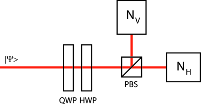
Figure 1: Apparatus for measuring the accessible density matrix for $N$ photon polarizations. The state $\ket{\Psi}$ is sent into a quarter waveplate (QWP) and half waveplate (HWP) followed by a polarizing beamsplitter (PBS). Number resolving photon counters count the number of vertical photons $N_{V}$ and the number of horizontal photons $N_{H}$.

We have shown that elements of the accessible density matrix offer the most complete description of the state of $N$ particles when one degree of freedom of the particles is visible and others are hidden. It is not clear from our discussion so far that it is possible to measure $\rho_{\text{acc}}$ using available experimental tools. In this section we will show that in the case of polarization it is indeed possible to measure $\rho_{\text{acc}}$ with a simple experimental device. This device, shown in figure 1, involves four different optical elements, a quarter wave-plate, a half-waveplate, a polarizing beamsplitter (PBS) and number-resolving photon counters (such as the one demonstrated in Achilles et al. (2003)) at the two ports. The multiphoton polarization state passes through the two waveplates and on to the PBS where it is split into $H$ and $V$ components. The number of photons in each port is then measured with the number-resolving single photon detector. Such a device is completely analogous to the Stern-Gerlach device for measuring spin projections.

If there are $N$ photons in the state then there are $N+1$ different ways that these can split between the $H$ and $V$ ports of the polarizing beamsplitter. When the photons leaving each port are counted, the measurement implemented will be a convex sum of projectors onto all states having that number of horizontal and vertical photons. For example, ${\mathbf{P}}_{N}=\ket{HH\cdots H}\bra{HH\cdots H}$, ${\mathbf{P}}_{N-1}=\left(\ket{VH\cdots H}\bra{VH\cdots H}+\ket{HV\cdots H}\bra{HV\cdots H}+\ldots\right)$, and so on. In angular momentum language ${\mathbf{P}}_{N}$ is a pure projector onto the state $j=N/2$, $m=N/2$. By changing the angles of the waveplates one can ‘orbit’ this measurement in the $j=N/2$ space thereby obtaining all the density matrix elements lying in the $j=N/2$ space. All $j=N/2$ matrix elements can be determined by measuring only rotated versions of ${\mathbf{P}}_{N}$. ${\mathbf{P}}_{N-1}$ is a convex sum of projectors onto all states with $m=N/2-1$. Since the $j=N/2$, $m=N/2-1$ projection can be determined from rotated versions of ${\mathbf{P}}_{N}$, we can subtract this part from ${\mathbf{P}}_{N-1}$ leaving a projector with support only in the $j=N/2-1$ subspace. By changing the waveplate angles one can use this reduced operator to completely characterize the $j=N/2-1$ space. One can then subtract the $j=N/2$ and $j=N/2-1$ terms from the $m=N/2-2$ operator, and so on. In this way all the terms in the accessible density matrix can be measured.

It should be noted that this is not the only way to measure the accessible density matrix. In fact any set of linearly independent measurements equal in number to the number of accessible density matrix elements as calculated from equation 7 can be used to reconstruct the accessible density matrix. Standard inversion techniques such as linear inversion, maximum likelihood fittingJames et al. (2001) and convex maximum likelihood fittingKosut et al. (2004) can be used to obtain $\rho_{\text{acc}}$ from an experimental dataset.

IV.1 Three-photon example

In this section we work through an example of how our techniques might be applied in a three-photon polarization experiment. We consider an experimental situation similar to the one used to create the state $\frac{1}{\sqrt{2}}\left(\ket{3_{H},0_{V}}+\ket{0_{H},3_{V}}\right)$ in reference Mitchell et al. (2004). There three photons were combined on a beamsplitter and post-selection was used to isolate those instances where all three photons left from the same port of the beamsplitter. If all the photons were indistinguishable, and each photon was set to the correct polarization then by this procedure the entangled state $\ket{3,0:0,3}=\frac{1}{\sqrt{2}}\left(\ket{3_{H},0_{V}}+\ket{0_{H},3_{V}}\right)$ would have been. This comes about because of the state is factorizable in raising operators through the relation:

$$\left(\right.{a^{\dagger}_{H}}^{3}+ {a^{\dagger}_{V}}^{3}\left.\right)$$

$$=\left(a^{\dagger}_{H}+a^{\dagger}_{V}\right)\left(a^{\dagger}_{H}+e^{2\pi i/3}a^{\dagger}_{V}\right)\left(a^{\dagger}_{H}+e^{4\pi i/3}a^{\dagger}_{V}\right)$$ (26)

Note that the right side is a product of polarization raising operators all acting on the same spatio-temporal mode.

In that experiment, however, two of the photons were produced by a spontaneous parametric downconversion process and the third was produced by an attenuated laser pulse. It is to be expected that these different sources might produce photons with hidden differences in their time-frequency wavefunctions. In principle such differences can be reduced by filtering, but let us suppose that filtering is insufficient, resulting in the mode of the third photon having only a 50% overlap with the mode of the other two photons, which are identical to one another. We can model this by replacing the raising operators in the third bracket in equation 26 with operators $c^{\dagger}_{H/V}=\frac{1}{\sqrt{2}}\left(a^{\dagger}_{H/V}+b^{\dagger}_{H/V}\right)$ where $b^{\dagger}$ is a creation operator for a mode $b$ orthogonal to the mode of $a$ for which $a^{\dagger}$ is the raising operator. The $50\%$ overlap is chosen here to keep the calculation simple. For a more general situation one can repeat the analysis using $c^{\dagger}_{H/V}=\cos{\theta}a^{\dagger}_{H/V}+\sin{\theta}b^{\dagger}_{H/V}$ where $\theta$ is an angle parametrizing the degree of overlap.

Inserting this substitution into equation 26, we obtain the expression

$$\frac{1}{\sqrt{11}} \left(a^{\dagger}_{H}+a^{\dagger}_{V}\right)\left(a^{\dagger}_{H}+e^{2\pi i/3}a^{\dagger}_{V}\right)\left(c^{\dagger}_{H}+e^{4\pi i/3}c^{\dagger}_{V}\right)$$

$$= \frac{1}{\sqrt{11}}\left[{a^{\dagger}_{H}}^{3}+{a^{\dagger}_{V}}^{3}\right]+\frac{1}{\sqrt{22}}\left[\right.{a^{\dagger}_{H}}^{2}b^{\dagger}_{H}+a^{\dagger}_{H}a^{\dagger}_{V}b^{\dagger}_{H}\left(1+e^{2\pi i/3}\right)$$

$$+{a^{\dagger}_{V}}^{2}b^{\dagger}_{H}e^{2\pi i/3}+{a^{\dagger}_{H}}^{2}b^{\dagger}_{V}e^{4\pi i/3}+a^{\dagger}_{H}a^{\dagger}_{V}b^{\dagger}_{V}\left(1+e^{4i\pi/3}\right)$$

$$+{a^{\dagger}_{V}}^{2}b^{\dagger}_{V}\left.\right]$$ (27)

Our goal is to write the state as an accessible density matrix, purely in terms of polarization measurements that can be done without knowing anything about the differences between the hidden time-frequency degrees of freedom. To arrive at such an expression we will need to trace over the orthogonal hidden modes $a$ and $b$. To do so the expression must first be rewritten in a first-quantized notation that clarifies the imposed separation between the hidden and visible degrees of freedom. The full expression is too long to write here, but rewriting one of the terms should be enough to give a feel for the calculation.

Consider the term $a^{\dagger}_{H}a^{\dagger}_{V}b^{\dagger}_{V}$. In rewriting this in first-quantized form we need to use tensor products of state vectors on the hidden and visible degrees of freedom, keeping in mind that the indistinguishability of the particles means that any one of the three can be in mode $b$. We write it as follows:

$$a^{\dagger}_{H} a^{\dagger}_{V}b^{\dagger}_{V}=$$

$$\frac{1}{\sqrt{6}}\left[\right.\left(\ket{HVV}+\ket{VHV}\right)\ket{aab}+\left(\ket{HVV}+\ket{VVH}\right)\ket{aba}$$

$$+\left(\ket{VHV}+\ket{VVH}\right)\ket{baa}\left.\right]$$ (28)

The trace over the hidden degrees of freedom produces an incoherent sum over the density matrices for each bracketed polarization state since $\ket{baa}$, $\ket{aab}$ and $\ket{aba}$ are orthogonal. The resulting accessible density matrix describing this term is

$$\rho_{\text{acc}}=\left[\begin{array}[]{cccccccc}0&0&0&0&\lx@intercol\hfil\lx@intercol\\ 0&0&0&0&\lx@intercol\hfil\lx@intercol\\ 0&0&2/3&0&\lx@intercol\hfil\lx@intercol\\ 0&0&0&0&&&&\\ \lx@intercol\hfil\hfil\lx@intercol&0&0&&\\ \lx@intercol\hfil\lx@intercol&0&1/6&&\\ \lx@intercol\hfil\lx@intercol&&&0&0\\ &&&&&&0&1/6\end{array}\right]$$ (29)

In the same way we can obtain the accessible density matrix for the entire state in Equation 27.

$$\rho_{\text{acc}}=\left[\begin{array}[]{cccccccc}0.3636&0&0&0.3636&\lx@intercol\hfil\lx@intercol\\ 0&0&0&0&\lx@intercol\hfil\lx@intercol\\ 0.0&0&0&0&\lx@intercol\hfil\lx@intercol\\ 0.3636&0&0&0.3636&&&&\\ \lx@intercol\hfil\hfil\lx@intercol&0.0682&-0.0341-0.0590i&&\\ \lx@intercol\hfil\lx@intercol&-0.0341+0.0590i&0.0682&&\\ \lx@intercol\hfil\lx@intercol&&&0.0682&-0.0341-0.0590i\\ &&&&&&-0.0341+0.0590i&0.0682\end{array}\right]$$ (30)

Note that the partial distinguishability of the third photon results in $27\%$ of the population being in the $j=1/2$ spaces instead of the $j=3/2$ spaces. The fidelityJozsa (1994) of this state to the desired state $\ket{3,0:0,3}$ is 0.7273. The distinguishability of one of the photons can therefore make a significant difference in the overall quality of the state.

So far we have assumed that we know the exact behaviour of the hidden degrees of freedom for our state. Let us now instead assume the experimental situation in which we can do polarization measurements but do not know about the hidden degrees of freedom making one of the three photons different from the other two. We will use a detection apparatus like the one in figure 1. The quarter and half waveplates are set to the angles listed in the first two columns of table 1. This results in a number of detections for each measurement outcome as listed in the last four columns. The numbers were generated via Monte Carlo simulation of Poisson-distributed data arising from the density matrix in equation 30. It was assumed that on average 10,000 three-photon states were measured for each waveplate setting.

The set of measurement operators in table 1 is overcomplete, as can be verified by explicit calculations of the dimension of the vector space they span. The $48$ projectors span a space of $20$ linearly independent dimensions. As predicted by equation 7, this is the maximum number of independent measurable operators when polarization is the only visible degree of freedom.

QWP	HWP	$3/2$	$1/2$	$-1/2$	$-3/2$
$0^{\circ}$	$0^{\circ}$	3645	1459	1385	3586
$15^{\circ}$	$0^{\circ}$	2201	3953	1006	2703
$30^{\circ}$	$0^{\circ}$	275	7699	160	1932
$45^{\circ}$	$0^{\circ}$	905	5260	2904	904
$0^{\circ}$	$12.25^{\circ}$	2078	2042	3834	1975
$15^{\circ}$	$12.25^{\circ}$	2759	2388	2185	2673
$30^{\circ}$	$12.25^{\circ}$	2105	2693	4174	1108
$45^{\circ}$	$12.25^{\circ}$	420	6700	1459	1272
$0^{\circ}$	$22.5^{\circ}$	910	2741	5163	888
$15^{\circ}$	$22.5^{\circ}$	892	4226	3021	1899
$30^{\circ}$	$22.5^{\circ}$	1337	3838	3207	1550
$45^{\circ}$	$22.5^{\circ}$	1914	2043	6069	0

Table 1: Simulated results of measurement of the state $\ket{30:03}=\frac{1}{\sqrt{2}}\left(\ket{3_{H},0_{V}}+\ket{0_{H},3_{V}}\right)$ when the spatio-temporal wavepacket of one of the photons has a $50\%$ overlap with that of the other two. The first two columns give angles for the waveplates, and the last four give the number of counts observed for each of the four outcomes of a number-resolving measurement. These outcomes are labeled by the value of $m$ with the understanding that they include contributions from all spaces with $j\geq m$. For example the $m=1/2$ column corresponds to the measurement operator $\ket{HHV}\bra{HHV}+\ket{HVH}\bra{HVH}+\ket{VHH}\bra{VHH}$.

These twenty parameters can be arranged to form an accessible density matrix in the form of equation 6, with the 20 elements broken into a 16-element symmetric $j=3/2$ subspace and the remaining four elements representing an average over the two $j=1/2$ subspaces.

Once this form is assumed for the accessible density matrix, the data can be fit to it using maximum-likelihood fittingKosut et al. (2004). To perform the fit we use the free convex optimization package SeDumiSturm (1999) for Matlab. In order to measure the likelihood that a given density matrix gave rise to the dataset we calculate the log-likelihoodKosut et al. (2004). The density matrix that maximizes this function given the outcomes listed in table 1 is given below.

$$\rho_{\text{acc}}=\left[\begin{array}[]{cccccccc}{\scriptstyle 0.3626}&{\scriptstyle 0.0057+0.0033i}&{\scriptstyle 0.0001-0.0003i}&{\scriptstyle 0.3597+0.0010i}&&&&\\ {\scriptstyle 0.0057-0.0033i}&{\scriptstyle 0.0036}&{\scriptstyle-0.0006-0.0028i}&{\scriptstyle 0.0023-0.0040i}&&&&\\ {\scriptstyle 0.0001+0.0003i}&{\scriptstyle-0.0006+0.0028i}&{\scriptstyle 0.0023}&{\scriptstyle 0.0013-0.0023i}&&&&\\ {\scriptstyle 0.3597-0.0010i}&{\scriptstyle 0.0023+0.0040i}&{\scriptstyle 0.0013+0.0023i}&{\scriptstyle 0.3601}&&&&\\ &&&&{\scriptstyle 0.0686}&{\scriptstyle-0.0322-0.0597i}&&\\ &&&&{\scriptstyle-0.0322+0.0597i}&{\scriptstyle 0.0670}&&\\ &&&&&&{\scriptstyle 0.0686}&{\scriptstyle-0.0322-0.0597i}\\ &&&&&&{\scriptstyle-0.0322+0.0597i}&{\scriptstyle 0.0670}\end{array}\right]$$ (31)

This can be seen to be very close the the density matrix in equation 30, with the difference accounted for by the statistical noise in the measurements.

The measured non-zero population in the non-symmetric subspace indicates the presence of hidden distinguishing information. The detection of this population would allow an experimentalist to infer the presence of a hidden degree of freedom (in this case the time-frequency degree of freedom) distinguishing one of the photons from the other two. It will also be noted that to the extent that the photons are indistinguishable, they are indeed in the desired state. In other words, the errors have arisen solely from the distinguishing information, and not, say, from unknown polarization rotations. This is all valuable information useful in diagnosing problems with the experiment.

It should be emphasized that there is nothing special about the particular waveplate settings used in this example. The important thing is that the resulting measurement operators fully span the space of accessible density matrix elements. If this is the case then the maximum-likelihood problem is well-defined and guaranteed to converge to the unique solutionKosut et al. (2004).

V Using the accessible density matrix to infer fundamental distinguishability

One of the main reasons for characterizing an experimentally generated polarization state is to substantiate claims that a particular quantum state of light has been achieved. For nearly all quantum protocols only the $j=N/2$ symmetric states will be useful since all the other states involve unwanted correlations with the hidden degrees of freedom which, by definition, cannot be manipulated. Usually one makes the claim that all the photons in the state are ‘indistinguishable’ in the hidden degrees of freedom, meaning that they all occupy the same hidden state. Our technique provides the first general method for verifying this claim.

If, when the accessible density matrix is measured, all the population is found to be in the symmetric space then it must be true that the hidden degrees of freedom are also in symmetric states. If this were not true then the overall state could not have the requisite bosonic symmetry under permutation.

If, in addition, the purity of the visible state is unity then the hidden degrees of freedom are unentangled with the visible degrees of freedom. This means that all measurements on the visible degrees of freedom will be consistent with the photons all being in the same single-particle hidden state. This being the case, it makes sense to call the photons ‘indistinguishable’ in the conventional sense of the word.

This definition of indistinguishability is entirely consistent with the one proposed by Liu et al.Liu et al. (2006); Sun et al. (2006) but is more flexible because it is expressed in the density matrix formalism which transforms in a predictable way under various operations one might wish to perform on the state.

VI Conclusions

We have outlined a procedure for measuring the state of a system of particles spread over several experimental modes which may be entangled with hidden degrees of freedom. Our technique should be used to justify claims of production of ‘indistinguishable’ photons. It is the most complete description of the state possible when some degrees of freedom are hidden, and in particular it gives a more complete description of the state than previous characterization techniques such as those employed in Bogdanov et al. (2004b), Liu et al. (2006) or Sun et al. (2006). In addition to being complete, this characterization also has the advantage of producing a density matrix that can be used in the usual way to predict the outcome of all measurements. We expect this method to become the standard means of characterizing states of a fixed number of experimentally indistinguishable photons just as quantum state tomographyJames et al. (2001) has become the standard means of characterizing distinguishable photons. Indeed since the number of accessible measurements for experimentally indistinguishable photons only grows polynomially with the number of photons in the state, our technique should prove useful for much larger systems of photons than state tomography does for distinguishable photons.