Loss-Induced Limits to Phase Measurement Precision with Maximally Entangled States

Abstract

The presence of loss limits the precision of an approach to phase measurement using maximally entangled states, also referred to as NOON states. A calculation using a simple beam-splitter model of loss shows that, for all nonzero values $L$ of the loss, phase measurement precision degrades with increasing number $N$ of entangled photons for $N$ sufficiently large. For $L$ above a critical value of approximately 0.785, phase measurement precision degrades with increasing $N$ for all values of $N$. For $L$ near zero, phase measurement precision improves with increasing $N$ down to a limiting precision of approximately $1.018L$ radians, attained at $N$ approximately equal to $2.218/L$, and degrades as $N$ increases beyond this value. Phase measurement precision with multiple measurements and a fixed total number of photons $N_{T}$ is also examined. For $L$ above a critical value of approximately 0.586, the ratio of phase measurement precision attainable with NOON states to that attainable by conventional methods using unentangled coherent states degrades with increasing $N$, the number of entangled photons employed in a single measurement, for all values of $N$. For $L$ near zero this ratio is optimized by using approximately $N=1.279/L$ entangled photons in each measurement, yielding a precision of approximately $1.340\sqrt{L/N_{T}}$ radians.

1 NOON States and the Heisenberg Limit

The use of entangled states has been proposed [1]-[15]as a means of performing phase measurements with a precision $\delta\phi_{min}$ at the Heisenberg limit. In this limit, $\delta\phi_{min}$ scales as

$$\delta\phi_{min}\sim 1/N,$$ (1)

with increasing photon number $N$, rather than at the standard quantum limit

$$\delta\phi_{min}\sim 1/\sqrt{N}.$$ (2)

Entangled-state enhancements to related tasks such as frequency measurement and lithography have also been proposed [16]-[36]. Experiments implementing phase measurements and related tasks using entangled states have been performed for the cases of $N=2$ [37]-[50], $N=3$ [51] and $N=4$ [52].

Maximally entangled states, also referred to as NOON states [53], are states of the form

$$|N::0\rangle_{a,b}=\frac{1}{\sqrt{2}}\left(|N,0\rangle_{a,b}+|0,N\rangle_{a,b}\right),$$ (3)

where

$$|m,n\rangle_{a,b}=|m\rangle_{a}|n\rangle_{b},$$ (4)

and where $|m\rangle_{a}$ is a Fock state with $m$ quanta in mode $a$,

$$|m\rangle_{a}=\frac{1}{\sqrt{m!}}\left({\widehat{a}_{a}}^{\dagger}\right)^{m}|0\rangle_{a},$$ (5)

with ${\widehat{a}_{a}}^{\dagger}$ and $|0\rangle_{a}$ the usual creation operator and vacuum state for mode $a$. In interferometry, for example, modes $a$ and $b$ are different paths around the interferometer. The argument that NOON states allow phase measurement at the Heisenberg limit is as follows.

A phase shift of $\phi$ in mode $b$ changes the state (3) to

$$|N::0;\phi\rangle_{a,b}=\frac{1}{\sqrt{2}}\left(|N,0\rangle_{a,b}+\exp(iN\phi)|0,N\rangle_{a,b}\right).$$ (6)

The phase $\phi$ can be determined by measuring the operator [54, 55, 51]

$$\widehat{A}_{N}=|0,N\rangle_{a,b}\;\;\mbox{}_{a,b}\langle N,0|+|N,0\rangle_{a,b}\;\;\mbox{}_{a,b}\langle 0,N|.$$ (7)

In the state (6), the expectation value of the operator (7) is

$$\langle\widehat{A}_{N}\rangle_{\phi} = \mbox{}_{a,b}\langle N::0\;;\phi|\widehat{A}_{N}|N::0\;;\phi\rangle_{a,b}$$ (8)

$$= \cos(N\phi),$$

and its variance is

$$\mbox{Var}_{\phi}\widehat{A}_{N} = \mbox{}_{a,b}\langle N::0\;;\phi|\widehat{A}_{N}^{2}|N::0\;;\phi\rangle_{a,b}-\left(\mbox{}_{a,b}\langle N::0\;;\phi|\widehat{A}_{N}|N::0\;;\phi\rangle_{a,b}\right)^{2}$$ (9)

$$= \sin^{2}(N\phi).$$

The signal-to-noise ratio (SNR) for detecting a change $\delta\phi$ about a phase value $\phi_{0}$ is[56]

$$\mbox{SNR}=\left(\langle\widehat{A}_{N}\rangle_{\phi_{0}+\delta\phi}-\langle\widehat{A}_{N}\rangle_{\phi_{0}}\right)^{2}/\mbox{Var}_{\phi_{0}}\widehat{A}_{N}.$$ (10)

Using (8) and (9) in (10),

$$\mbox{SNR}=N^{2}\left(\delta\phi\right)^{2}$$ (11)

for small phase changes,

$$|\delta\phi|\ll 2\pi\/.$$ (12)

Defining the minimum detectable phase change $\delta\phi_{min}$ to be that phase change corresponding to an SNR of unity[57], (11) gives

$$\delta\phi_{min}=1/N.$$ (13)

Phase measurement by this method is thus seen to be at the Heisenberg limit (1), with a precision that can be increased arbitrarily by increasing $N$.

2 NOON-State Phase Measurement in the Presence of Loss

In any real system some photons will inevitably be lost prior to detection, a feature not represented in the model of phase measurement described above. Loss can be represented by including in the model fictitious beam splitters[58] through which photons in the state (6) pass before being subjected to the measurement (7). Having in mind potential application to laser radar with coherent detection[59], where one beam impinges directly on a detector while the other first suffers loss due to spreading during reflection from a distant target, we include a single such fictitious beam splitter, in mode $b$.

Denote by $\widehat{a}_{b}$ the mode operator at the input port to the fictitious beam splitter, by $\widehat{a}_{b^{\prime}}$ the mode operator at the output port of the beam splitter through which photons proceed to the detector, and by $\widehat{a}_{V}$ the mode operator at the other input port (vacuum port) of the beam splitter (see Fig. 1). These operators are related by[60]

$$\widehat{a}_{b^{\prime}}=t\widehat{a}_{b}+r\widehat{a}_{V}$$ (14)

with $t$ and $r$ the respective transmission and reflection coefficients. The loss $L$ which is thus represented is of magnitude

$$L=1-\eta,$$ (15)

where

$$\eta=|t|^{2}.$$ (16)

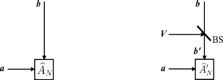
(a)                                            (b)

Figure 1: Input modes to phase measurement. (a) Without loss. (b) With loss in one mode, modeled by beam splitter BS.

The detection operator (7) becomes

$$\widehat{A}^{\prime}_{N}=|0,N\rangle_{a,b^{\prime}}\;\;\mbox{}_{a,b^{\prime}}\langle N,0|+|N,0\rangle_{a,b^{\prime}}\;\;\mbox{}_{a,b^{\prime}}\langle 0,N|.$$ (17)

The $a$ mode is unaffected by the presence of the beam splitter, and

$$|0\rangle_{b}\/=|0\rangle_{b^{\prime}},$$ (18)

since the beam splitter does not introduce additional photons into the system. Using (4), (5), (14), (17) and (18),

$$\widehat{A}_{N}^{\prime}=\frac{1}{\sqrt{N}}\left[\left(t^{\ast}\widehat{a}^{\dagger}_{b}+r^{\ast}\widehat{a}^{\dagger}_{V}\right)^{N}\left(|0,0\rangle_{a,b}\;\;\mbox{}_{a,b}\langle N,0|\right)+\left(|N,0\rangle_{a,b}\;\;\mbox{}_{a,b}\langle 0,0|\right)\left(t\widehat{a}_{b}+r\widehat{a}_{V}\right)^{N}\right].$$ (19)

The state space is now enlarged to include the fictitious beam splitter vacuum port mode $V$, so the state vector must include a factor of the vacuum state for that mode:

$$|N::0;\phi\rangle_{a,b,V}=|N::0;\phi\rangle_{a,b}|0\rangle_{V}.$$ (20)

Using (6), (16), (19) and (20), and defining

$$\theta_{t}=\arg t,$$ (21)

we obtain

$$\langle\widehat{A}^{\prime}_{N}\rangle_{\phi} = \mbox{}_{a,b,V}\langle N::0;\phi|\widehat{A}^{\prime}_{N}|N::0;\phi\rangle_{a,b,V}$$ (22)

$$= \eta^{N/2}\cos(N(\phi+\theta_{t}))$$

and

$$\mbox{Var}_{\phi}\widehat{A}^{\prime}_{N} = \mbox{}_{a,b,V}\langle N::0;\phi|\left(\widehat{A}^{\prime}_{N}\right)^{2}|N::0;\phi\rangle_{a,b,V}-\left(\mbox{}_{a,b,V}\langle N::0;\phi|\widehat{A}^{\prime}_{N}|N::0;\phi\rangle_{a,b,V}\right)^{2}$$ (23)

$$= \frac{1}{2}\left(1+\eta^{N}\right)-\eta^{N}\cos^{2}\left(N(\phi+\theta_{t})\right).$$

The signal-to-noise ratio for detecting a small change of phase $\delta\phi$ in the presence of loss, is, using (22) and (23),

$$\mbox{SNR}^{\prime} = \left(\langle\widehat{A}^{\prime}_{N}\rangle_{\phi_{0}+\delta\phi}-\langle\widehat{A}^{\prime}_{N}\rangle_{\phi_{0}}\right)^{2}/\mbox{Var}_{\phi_{0}}\widehat{A}^{\prime}_{N}$$ (24)

$$= \frac{N^{2}\sin^{2}(N(\phi_{0}+\theta_{t}))\left(\delta\phi\right)^{2}}{\frac{1}{2}\left(\eta^{-N}+1\right)-\cos^{2}(N(\phi_{0}+\theta_{t}))}.$$

The minimum detectable phase change in the presence of loss, that value of $\delta\phi$ for which $\mbox{SNR}^{\prime}$ in (24) is unity, is therefore

$$\delta\phi^{\prime}_{min}=\frac{\left[\frac{1}{2}\left(\eta^{-N}+1\right)-\cos^{2}(N(\phi_{0}+\theta_{t}))\right]^{1/2}}{N|\sin(N((\phi_{0}+\theta_{t}))|}.$$ (25)

In the absence of loss, i.e. for $\eta=1$, (25) agrees with (13). For fixed $\eta<1$ and $N$, (25) is minimized for values of $\phi_{0}+\theta_{t}$ such that

$$N(\phi_{0}+\theta_{t})=(n+1/2)\pi,\hskip 14.22636ptn=0,\pm 1,\pm 2,\ldots$$ (26)

Since we wish to model pure loss we will take the transmission coefficient of the fictitious beam splitter to be real, so

$$\theta_{t}=0.$$ (27)

Imposing (27) and assuming that $\phi_{0}$ satisfies (26), (25) becomes

$$\delta\phi^{\prime}_{min}=\frac{\sqrt{\left(\eta^{-N}+1\right)/2}}{N}.$$ (28)

This result agrees with that obtained previously by Chen et al. [61] using a master-equation model of continuous loss and entanglement. For any nonzero amount of loss, i.e., for $\eta<1$, we see from (28) that

$$\lim_{N\rightarrow\infty}\delta\phi^{\prime}_{min}=\infty.$$ (29)

3 The Small-Loss and Large-Loss Cases

The behavior of $\delta\phi^{\prime}_{min}$ for varying $N$ and $\eta$, as given exactly in (28), is of particular interest in two limiting cases: very large amounts of loss, $L\raisebox{-2.58334pt}{$\,\stackrel{{\scriptstyle\raisebox{-0.60275pt}{$\textstyle<$}}}{{\sim}}\,$}1$, $\eta\ll 1$, and very small amounts of loss, $L\ll 1$, $\eta\raisebox{-2.58334pt}{$\,\stackrel{{\scriptstyle\raisebox{-0.60275pt}{$\textstyle<$}}}{{\sim}}\,$}1$. The large-loss limit is relevant for laser radar, while the limit of small loss, on the other hand, is relevant for precision laboratory experiments and technological applications.

Consider first the case of large loss. From (28),

$$\frac{d\delta\phi^{\prime}_{min}}{dN}=-\frac{1}{N^{2}}\left[\left(\eta^{-N}+1\right)/2\right]^{1/2}-\frac{\eta^{-N}\log\eta}{4N}\left[\left(\eta^{-N}+1\right)/2\right]^{-1/2},$$ (30)

so

$$\lim_{\eta\rightarrow 0}\frac{d\delta\phi^{\prime}_{min}}{dN}=\frac{-\log\eta\;\eta^{N/2}}{4\sqrt{2}N}$$ (31)

which for $\eta<1$ is strictly positive for all $N$. So increasing $N$ can only harm the precision of phase measurement in this limit, and there is no $N$ for which the detector can provide useful results satisfying (12). See Fig. 2(a).

In the limit of small loss, as exemplified in Fig. 2(b), we can estimate the smallest possible $\delta\phi^{\prime}_{min}$, and the value of $N$ at which it is obtained, as follows. From (28),

$$\frac{d}{dN}\log\delta\phi^{\prime}_{min}=-\frac{1}{N}-\frac{\log\eta}{2\left(\eta^{N}+1\right)},$$ (32)

so

$$N_{min}(\eta)=\frac{-2\left(\eta^{N_{min}(\eta)}+1\right)}{\log\eta},$$ (33)

where $N_{min}(\eta)$ is that $N$ which minimizes $\delta\phi^{\prime}_{min}$ for a given $\eta$. We look for $N_{min}(\eta)$ of the form

$$\lim_{L\rightarrow 0}N_{min}(\eta)=\frac{\nu}{L}.$$ (34)

Using (34) in (33), we obtain

$$\frac{\nu}{L}=\lim_{L\rightarrow 0}\frac{-2\left((1-L)^{\frac{\nu}{L}}+1\right)}{-L},$$ (35)

or

$$\nu=2\left(e^{-\nu}+1\right)$$ (36)

which may be solved numerically to obtain

$$\nu\approx 2.218.$$ (37)

Using (34) in (28)

$$\lim_{L\rightarrow 0}\delta\phi^{\prime}_{min}\;\rule[-5.69054pt]{0.28453pt}{19.91692pt}_{N=N_{min}(\eta)}=\mu L,$$ (38)

where

$$\mu = \lim_{L\rightarrow 0}\frac{1}{\nu}\left[\frac{1}{2}\left((1-L)^{-\frac{\nu}{L}}+1\right)\right]^{1/2}$$ (39)

$$= \frac{1}{\nu}\left[\frac{1}{2}\left(e^{\nu}+1\right)\right]^{1/2}$$

$$\approx 1.018.$$

using (37). For $L$ as large as .01 the expressions (34) and (38) give values within a percent of the exact values obtained from (28).

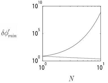
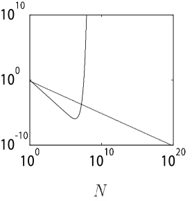
(a)                                            (b)

Figure 2: $\delta\phi^{\prime}_{min}$ (curved lines) as a function of $N$. (a) $L=.99$. (b) $L=10^{-6}$. Straight lines are the function $1/\sqrt{2\eta N}$, where $\eta=1-L.$

To find the critical value of loss $L=L_{c}$ above which $\delta\phi^{\prime}_{min}$ must be a nondecreasing function of $N$, we first examine the cases $N=1$ and $N=2$. For $\delta\phi^{\prime}_{min}$ to be smaller at $N=2$ than at $N=1$, we find from (28) that we must have

$$\eta>\eta_{c},$$ (40)

where

$$\eta_{c}=\frac{\sqrt{7}-2}{3}\approx 0.215.$$ (41)

From this it follows that, if $\eta\leq\eta_{c}$, then $\delta\phi^{\prime}_{min}$ will not be smaller than its value at $N=2$ for any value of $N$. For, if $\delta\phi^{\prime}_{min}$ were to be smaller for some $N>2$ than for $N=2$, it would be necessary for

$$\frac{d\delta\phi^{\prime}_{min}}{dN}<0$$ (42)

to hold for some value of $N\geq 2$. Using (30), this means that for some $N\geq 2$,

$$\log\eta>\frac{-2}{N}\left(\eta^{N}+1\right).$$ (43)

But $\eta\leq\eta_{c}$, so (43) implies

$$\log\eta>\frac{-2}{N}\left({\eta_{c}}^{N}+1\right)$$ (44)

and

$$\log\eta_{c}>\frac{-2}{N}\left({\eta_{c}}^{N}+1\right).$$ (45)

So,

$$N<\frac{-2\left({\eta_{c}}^{N}+1\right)}{\log\eta_{c}},$$ (46)

implying

$$N<\frac{-2\left({\eta_{c}}+1\right)}{\log\eta_{c}}$$ (47)

since $\eta_{c}<1$ and $N\geq 2$. Using (47) and (41), we obtain

$$N\raisebox{-2.58334pt}{$\,\stackrel{{\scriptstyle\raisebox{-0.60275pt}{$\textstyle<$}}}{{\sim}}\,$}1.582,$$ (48)

contradicting the requirement $N\geq 2$. So $\delta\phi^{\prime}_{min}$ will be a nondecreasing function of $N$ whenever

$$L>L_{c},$$ (49)

where

$$L_{c}=1-\eta_{c}\approx 0.785.$$ (50)

4 Comparison With Unentangled Phase Measurement; Multiple Measurements

For phase estimation with unentangled coherent light and homodyne or heterodyne detection[58], we would expect a precision of $\kappa/\sqrt{\eta N}$ in the presence of loss, where $\kappa$ is independent of $N$ and of order unity. No matter how large the loss, this precision can always be improved by increasing $N$, and thus can always surpass the precision attainable with NOON states and a detector implementing the operator (7). (It is conceivable that detectors implementing other measurement operators, with nonvanishing matrix elements between states other than just linear combinations of $|N,0\rangle_{a,b}$ and $|0,N\rangle_{a,b}$, might be less sensitive to loss while still surpassing the standard quantum limit (2), but we have not investigated this issue here.) If in a particular application with small loss there is a limit to how large $N$ can be, and if this limit is not much larger than that given by (34), (37), then the use of NOON states with (7) can lead to precision better than that attainable with standard techniques. See Fig. 2(b).

The analysis up to this point has been based on phase measurements using individual quantum states with $N$ photons. If the measurements are repeated $M$ times, using $M$ independent quantum states, the minimum detectable phase change will decrease by an additional factor of $1/\sqrt{M}$. For measurement with unentangled coherent-state photons, the precision will be

$$\delta\phi_{un}=\kappa/\sqrt{\eta NM}=\kappa/\sqrt{\eta N_{T}},$$ (51)

where

$$N_{T}=NM$$ (52)

is the average total number of photons available. That is, for phase measurements with unentangled coherent light we obtain the same precision whether we make many measurements with fewer photons per measurement or fewer measurements with more photons per measurement.

For NOON-state photons, the precision after $M$ $N$-photon measurements is

$$\delta\phi_{NOON} = \delta\phi^{\prime}_{min}/\sqrt{M}$$ (53)

$$= \sqrt{\frac{\eta^{-N}+1}{2NN_{T}}}$$

using (28) and (52), or

$$\delta\phi_{NOON}=R_{NOON}/\sqrt{\eta N_{T}},$$ (54)

where $R_{NOON}$ is, aside from the constant factor $\kappa$, the ratio of NOON phase measurement precision to unentangled phase precision (51) with equal $L$ and $N_{T}$,

$$R_{NOON}=\sqrt{\frac{\eta(\eta^{-N}+1)}{2N}}.$$ (55)

Graphs of $R_{NOON}$ as a function of $N$ are presented in Fig. 3 for $L=.99$ and $L=10^{-6}$.

For fixed $N_{T}$, $\delta\phi_{un}$ is constant, and $\delta\phi_{NOON}$ is minimized by minimizing $R_{NOON}$ as a function of the number $N$ of photons per NOON state. Denote the minimizing value of $N$ by $\widetilde{N}_{min}(\eta)$. For large loss, $L\raisebox{-2.58334pt}{$\,\stackrel{{\scriptstyle\raisebox{-0.60275pt}{$\textstyle<$}}}{{\sim}}\,$}1$, we find from (55) that

$$\lim_{\eta\rightarrow 0}\frac{dR_{NOON}}{dN}=\frac{-\log\eta\;\eta^{-\left(\frac{N-1}{2}\right)}}{8\sqrt{2N}}$$ (56)

which is strictly positive for all $N$. (See, e.g., Fig. 3(a).) So

$$\lim_{L\rightarrow 1}\widetilde{N}_{min}(\eta)=1,$$ (57)

which with (53) yields

$$\lim_{L\rightarrow 1}\delta\phi_{NOON}\;\rule[-5.69054pt]{0.28453pt}{19.91692pt}_{\;N=\widetilde{N}_{min}(\eta)}=1/\sqrt{2\eta N_{T}}.$$ (58)

The phase measurement precision obtainable with NOON states is thus, in the large-loss limit, the same as that obtainable with unentangled coherent states, eq. (51), up to a constant factor.

In the complete absence of loss, i.e. for $\eta=1$, $R_{NOON}=1/\sqrt{N}$ and is minimized by making $N$ as large as possible,

$$\widetilde{N}_{min}(\eta)\;\rule[-5.69054pt]{0.28453pt}{19.91692pt}_{\;L=0}=N_{T}.$$ (59)

That is, for $L=0$ the greatest precision using the NOON-state measurement scheme (7) and a fixed total number of photons $N_{T}$ is obtained by making a single measurement with all $N_{T}$ photons. Using (59) and $\eta=1$ in (53),

$$\delta\phi_{NOON}\;\rule[-5.69054pt]{0.28453pt}{19.91692pt}_{\;N=N_{min}(\eta),L=0}=1/N_{T}.$$ (60)

Using $\eta=1$ in (51),

$$\delta\phi_{un}\;\rule[-5.69054pt]{0.28453pt}{19.91692pt}_{\;L=0}=\kappa/\sqrt{N_{T}}.$$ (61)

Comparing (60) and (61) we see that, in the absence of loss, the improvement in phase measurement precision obtained by using NOON states is of order $\sqrt{N_{T}}$, as expected.

For small loss, $\eta\raisebox{-2.58334pt}{$\,\stackrel{{\scriptstyle\raisebox{-0.60275pt}{$\textstyle<$}}}{{\sim}}\,$}1$, an analysis along the lines of Sec. 3 gives

$$\lim_{L\rightarrow 0}\widetilde{N}_{min}(\eta)=\frac{\widetilde{\nu}}{L},$$ (62)

where $\widetilde{\nu}$ is the solution to

$$\widetilde{\nu}=e^{-\widetilde{\nu}}+1,$$ (63)

which is found numerically to be

$$\widetilde{\nu}\approx 1.279.$$ (64)

The corresponding minimum value of $\delta\phi_{NOON}$ is

$$\lim_{L\rightarrow 0}\delta\phi_{NOON}\;\rule[-5.69054pt]{0.28453pt}{19.91692pt}_{\;N=\widetilde{N}_{min}(\eta)}=\widetilde{\mu}\sqrt{L/N_{T}},$$ (65)

where

$$\widetilde{\mu}=\sqrt{\frac{e^{\widetilde{\nu}}+1}{2\widetilde{\nu}}}\approx 1.340.$$ (66)

Comparing (65) with (51), we see that, when $L\raisebox{-2.58334pt}{$\,\stackrel{{\scriptstyle\raisebox{-0.60275pt}{$\textstyle>$}}}{{\sim}}\,$}0$, NOON states give an improvement in phase measurement precision of order $\sqrt{L}$.

(In the limit of zero loss, (62) indicates that $R_{NOON}$ has a local minimum at $\widetilde{N}_{min}(1)=\infty$, corresponding according to (65) to $\delta\phi_{NOON}=0$. But, of course, $N$ cannot be made larger than $N_{T}$, corresponding to the results (59), (60) in the lossless case.)

An analysis along the lines of Sec. 3 shows that $R_{NOON}$, and therefore $\delta\phi_{NOON}$ for fixed $N_{T}$, is an increasing function of $N$ for all $L>\widetilde{L}_{c}$, where

$$\widetilde{L}_{c}=2-\sqrt{2}\approx 0.586.$$ (67)

It is not surprising that $\widetilde{L}_{c}$ is lower than $L_{c}$ since, in the multiple-measurement case, increasing $N$, even when it decreases the single-measurement precision $\delta\phi^{\prime}_{min}$, increases the factor $1/\sqrt{M}=\sqrt{N_{T}/N}$ which enters into $\delta\phi_{NOON}$, eq. (53).

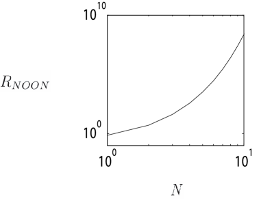
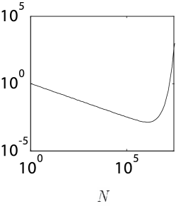
(a)                                            (b)

Figure 3: $R_{NOON}$ as a function of $N$. (a) $L=.99$. (b) $L=10^{-6}$.

References

- [1] Yurke, B., “Input states for enhancement of fermion interferometer sensitivity,” Phys. Rev. Lett. 56, 1515-1517 (1986).
- [2] Yurke, B., McCall, S. L. and Klauder, J. R., “SU(2) and SU(1,1) interferometers,” Phys. Rev. A 33, 4033-4054 (1986).
- [3] Kitagawa, M. and Ueda, M., “Nonlinear-interferometric generation of number-phase-correlated fermion states,” Phys. Rev. Lett. 67 1852-1854 (1991).
- [4] Kitagawa, M. and Ueda, M., “Squeezed spin states,” Phys. Rev. A 47, 5138-5143 (1993).
- [5] Holland, M. J. and Burnett, K., “Interferometric detection of optical phase shifts at the Heisenberg limit,” Phys. Rev. Lett. 71, 1355-1358 (1993).
- [6] Sanders, B. C. and Milburn, G. J. “Optimal quantum measurements for phase estimation,” Phys. Rev. Lett. 75, 2944-2947 (1995).
- [7] Jacobson, J., Björk. G. and Yamamoto, Y., “Quantum limit for the atom-light interferometer,” Appl. Phys. B 60, 187-191 (1995).
- [8] Ou, Z. Y., “Complementarity and fundamental limit in precision phase measurement,” Phys. Rev. Lett. 77, 2352-2355 (1996).
- [9] Ou, Z. Y., “Fundamental quantum limit in precision phase measurement,” Phys. Rev. A 55, 2598-2609 (1997).
- [10] Bouyer, P. and Kasevich, M. A., “Heisenberg-limited spectroscopy with degenerate Bose-Einstein gases,” Phys. Rev. A 56, R1083-R1086 (1997).
- [11] Dowling, J.P., “Correlated input-port, matter-wave interferometer: Quantum noise limits to the atom-laser gyroscope,” Phys. Rev. A 57, 4736-4746 (1998).
- [12] Gerry, C. C., “Heisenberg-limit interferometry with four-wave mixers operating in a nonlinear regime,” Phys. Rev. A 61, 043811 (2000).
- [13] Gerry, C. C., Benmoussa, A. and Campos, R. A., “Nonlinear interferometer as a resource for maximally entangled photonic states: Application to interferometry,” Phys. Rev. A 66, 013804 (2002).
- [14] Campos, R. A., Gerry, C. C. and Benmoussa, A., “Optical interferometry at the Heisenberg limit with twin Fock states and parity measurements,” Phys. Rev. A 68, 023810 (2003).
- [15] Lee, H., Kok, P., Williams, C. P. and Dowling, J. P., “From linear optical quantum computing to Heisenberg-limited interferometry,” J. Opt. B 6 S796 S800 (2004).
- [16] Wineland, D. J., Bollinger, J. J., Itano, W. M., Moore, F. L. and Heinzen, D. J., “Spin squeezing and reduced quantum noise in spectroscopy,” Phys. Rev. A 46, R6797-R6800 (1992).
- [17] Agarwal, G. S. and Puri, R. R., “Atomic states with spectroscopic squeezing, ” Phys. Rev. A 49, 4968-4971 (1994).
- [18] Wineland, D. J., Bollinger, J. J., Itano, W. M. and Heinzen, D. J., “Squeezed atomic states and projection noise in spectroscopy,” Phys. Rev. A 50, 67-88 (1994).
- [19] Bollinger, J. J., Itano, W. M., Wineland, D. J. and Heinzen, D.J., “Optimal frequency measurements with maximally correlated states,” Phys. Rev. A 54 R4649-R4652 (1996).
- [20] Yablonovitch, E. and Vrijen, R. B., “Optical projection lithography at half the Rayleigh resolution limit by two-photon exposure,” Opt. Eng. 38, 334-338 (1999).
- [21] Boto, A. N., Kok, P., Abrams, D. S., Braunstein, S. L., Williams, C. P. and Dowling, J. P., “Quantum interferometric optical lithography: Exploiting entanglement to beat the diffraction limit,” Phys. Rev. Lett. 85, 2733-2736 (2000).
- [22] Kok, P., Boto, A. N., Abrams, D. S., Williams, C. P., Braunstein, S. L. and Dowling, J. P., “Quantum-interferometric optical lithography: Towards arbitrary two-dimensional patterns,” Phys. Rev. A 63, 063407 (2001).
- [23] Nagasako, E. M., Bentley, S. J., Boyd, R .W. and Agarwal, G. S., “Nonclassical two-photon interferometry and lithography with high-gain parametric amplifiers,” Phys. Rev. A 64, 043802 (2001).
- [24] Gerry, C. C. and Campos, R. A., “Generation of maximally entangled photonic states with a quantum-optical Fredkin gate,” Phys. Rev. A 64, 063814 (2001).
- [25] Agarwal G. S., Boyd R. W., Nagasako, E. M. and Bentley, S. J., “Comment on ‘Quantum interferometric optical lithography: Exploiting entanglement to beat the diffraction limit,’ ”Phys. Rev. Lett. 86, 1389 (2001).
- [26] Giovannetti, V., Lloyd, S., Maccone, L. and Wong, F. N. C., “Clock synchronization with dispersion cancellation,” Phys. Rev. Lett. 87, 117902 (2001).
- [27] Giovannetti, V., Lloyd, S. and Maccone, L., “Quantum-enhanced positioning and clock synchronization,” Nature 412, 417-419 (2001).
- [28] Giovannetti, V., Lloyd, S. and Maccone, L., “Positioning and clock synchronization through entanglement,” Phys. Rev. A 65, 022309 (2002).
- [29] Gerry, C. C. and Benmoussa, A., “Heisenberg-limited interferometry and photolithography with nonlinear four-wave mixing,” Phys. Rev. A 65, 033822 (2004).
- [30] Giovannetti, V., Lloyd, S. and Maccone, L., “Quantum cryptographic ranging,” J. Opt. B 4, S413-S414 (2002).
- [31] Giovannetti, V., Lloyd, S., Maccone, L. and Wong, F. N. C., “Clock synchronization and dispersion,” J. Opt. B 4, S415-S417 (2002).
- [32] Agarwal, G. S. and Scully, M. O., “Magneto-optical spectroscopy with entangled photons,” Opt. Lett. 28, 462-464 (2003).
- [33] Muthukrishnan, A., Scully, M. O., and Zubairy, M. S., “Quantum microscopy using photon correlations,” J. Opt. B 6, S575-S582 (2004).
- [34] Giovannetti, V., Lloyd, S. and Maccone, L., “Quantum-enhanced measurements: Beating the standard quantum limit,” Science 306, 1330-1336 (2004).
- [35] Giovannetti, V., Lloyd, S. and Maccone, L., “Quantum metrology,” Phys. Rev. Lett. 96, 010401 (2006).
- [36] Kapale, K. T. and Dowling, J. P., “A bootstrapping approach for generating maximally path-entangled photon states,” quant-ph/0612196.
- [37] Ou, Z. Y., Wang, L. J., Zou, X. Y. and Mandel, L., “Evidence for phase memory in two-photon down conversion through entanglement with the vacuum, Phys. Rev. A 41, 566-568 (1990).
- [38] Rarity, J. G., Tapster, P. R., Jakeman, E., Larchuk, T., Campos, R. A., Teich, M. C. and Saleh, B. E. A., “Two-photon interference in a Mach-Zehnder interferometer,” Phys. Rev. Lett. 65, 1348-1351 (1990).
- [39] Kwiat, P. G., Vareka, W. A., Hong, C. K., Nathel, H. and Chiao, R. Y., “Correlated two-photon interference in a dual-beam Michelson interferometer,” Phys. Rev. A 41 2910-2913 (1990).
- [40] Ou, Z. Y., Zou, X. Y., Wang, L. J. and Mandel, L., “Experiment on nonclassical fourth-order interference,” Phys. Rev. A 42, 2957-2965 (1990).
- [41] Steinberg, A. M., Kwiat, P. G. and Chiao, R. Y., “Dispersion cancellation in a measurement of the single-photon propagation velocity in glass,” Phys. Rev. Lett., 68, 2421-2424 (1992).
- [42] Steinberg, A. M., Kwiat, P. G. and Chiao, R. Y., “Dispersion cancellation and high-resolution time measurements in a fourth-order optical interferometer,” Phys. Rev. A 45, 6659-6665 (1992).
- [43] Fonseca, E. J. S., Monken, C. H. and Pádua, S., “Measurement of the de Broglie wavelength of a multiphoton wave packet,” Phys. Rev. Lett. 82, 2868-2871 (1999).
- [44] Fonseca, E. J. S., Monken, C. H., Pádua, S. and Barbosa, G. A., “Transverse coherence length of down-converted light in the two-photon state,” Phys. Rev. A 59, 1608-1614 (1999).
- [45] Fonseca, E. J. S., Souto Ribeiro, P. H., Pádua, S. and Monken, C. H., “Quantum interference by a nonlocal double slit,” Phys. Rev. A 60, 1530-1533 (1999).
- [46] Fonseca, E. J. S., Machado da Silva, J. C., Monken, C. H. and Pádua, S., “Controlling two-particle conditional interference,” Phys. Rev. A 61, 023801 (2000).
- [47] Fonseca, E. J. S., Paulini, Z., Nussenzveig, P., Monken, C. H. and Pádua, S., “Nonlocal de Broglie wavelength of a two-particle system,” Phys. Rev. A 63, 043819 (2001).
- [48] D’Angelo, M., Chekhova, M. V. and Shih, Y., “Two-photon diffraction and quantum lithography,” Phys. Rev. Lett. 87, 013602 (2001).
- [49] Edamatsu, K., Shimizu, R. and Itoh, T., “Measurement of the photonic de Broglie wavelength of entangled photon pairs generated by spontaneous parametric down-conversion,” Phys. Rev. Lett. 89, 213601 (2002).
- [50] Bennink, R. S., Bentley, S. J. and Boyd, R. W., “Quantum and classical coincidence imaging,” Phys. Rev. Lett. 92, 033601 (2004)
- [51] Mitchell, M. W., Lundeen, J. S., and Steinberg, A. M., “Super-resolving phase measurements with a multiphoton entangled state,” Nature 429, 161-164 (2004).
- [52] Walther, P., Pan, J. -W., Aspelmeyer, M., Ursin, R., Gasparoni, S. and Zeilinger, A., “De Broglie wavelength of a non-local four-photon state,” Nature 429, 158-161.
- [53] Gerry, C. C. and Knight, P. L. Introductory Quantum Optics (Cambridge, 2005).
- [54] Kok, P., Lee, H. and Dowling, J. P., “Creation of large-photon-number path entanglement conditioned on photodetection,” Phys. Rev. A 65, 052104 (2002).
- [55] Lee, H., Kok, P. and Dowling, J. P., “A quantum Rosetta stone for interferometry,” J. Mod. Opt. 49, 2325-2338 (2002).
- [56] Helstrom, C. W., Quantum Detection and Estimation Theory (Academic, New York, 1976).
- [57] Walls, D. F. and Milburn, G. J., Quantum Optics (Springer, Berlin, 1994).
- [58] Gardiner, C. W. and Zoller, P., Quantum Noise, 3d ed. (Springer, Berlin, 2004).
- [59] Kingston, R. H., Optical Sources, Detectors, and Systems, (Academic, San Diego, 1995).
- [60] Gottfreid, K. and Yan, T.-M., Quantum Mechanics: Fundamentals, 2nd ed. (Springer, New York, 2003).
- [61] Chen, X.-Y., Jiang, L.-z. and Han, L., “The entanglement of damped noon-state and its performance in phase measurement,” quant-ph/0605184.