Linear optics and quantum maps

Abstract

We present a theoretical analysis of the connection between classical polarization optics and quantum mechanics of two-level systems. First, we review the matrix formalism of classical polarization optics from a quantum information perspective. In this manner the passage from the Stokes-Jones-Mueller description of classical optical processes to the representation of one- and two-qubit quantum operations, becomes straightforward. Second, as a practical application of our classical-vs-quantum formalism, we show how two-qubit maximally entangled mixed states (MEMS), can be generated by using polarization and spatial modes of photons generated via spontaneous parametric down conversion.

I Introduction

Quantum computation and quantum information have been amongst the most popular branches of physics in the last decade Nielsen and Chuang (2002). One of the reasons of this success is that the smallest unit of quantum information, the qubit, could be reliably encoded in photons that are easy to manipulate and virtually free from decoherence at optical frequencies Zeilinger (1999); Gisin et al. (2002). Thus, recently, there has been a growing interest in quantum information processing with linear optics Knill et al. (2001); O’Brien et al. (2003); Skaar et al. (2004); Kok and several techniques to generate and manipulate optical qubits have been developed for different purposes ranging from, e.g., teleportation Bouwmeester et al. (1997); Boschi et al. (1998), to quantum cryptography Gisin et al. (2002), to quantum measurements of qubits states James et al. (2001) and processes O’Brien et al. (2004), etc. In particular, Kwiat and coworkers Peters et al. (2003); Wei et al. (2005) were able to create and characterize arbitrary one- and two-qubit states, using polarization and frequency modes of photons generated via spontaneous parametric down conversion (SPDC) Yariv (1989).

Manipulation of optical qubits is performed by means of linear optical instruments such as half- and quarter-wave plates, beam splitters, polarizers, mirrors, etc., and networks of these elements. Each of these devices can be thought as an object where incoming modes of the electromagnetic fields are turned into outgoing modes by a linear transformation. From a quantum information perspective, this transforms the state of qubits encoded in some degrees of freedom of the incoming photons, according to a completely positive map $\mathcal{E}$ describing the action of the device. Thus, an optical instrument may be put in correspondence with a quantum map and vice versa. Such correspondence has been largely exploited Zhang (2004); Peters et al. (2003); Wei et al. (2005); Kok and stressed Brunner et al. (2003); Aiello et al. (2006) by several authors. Moreover, classical physics of linear optical devices is a textbook matter Born and Wolf (1999); Damask (2005), and quantum physics of elementary optical instruments has been studied extensively Leonhardt (2003), as well. However, surprisingly enough, a systematic exposition of the connection between classical linear optics and quantum maps is still lacking.

In this paper we aim to fill this gap by presenting a detailed theory of linear optical instruments from a quantum information point of view. Specifically, we establish a rigorous basis of the connection between quantum maps describing one- and two-qubit physical processes operated by polarization-affecting optical instruments, and the classical matrix formalism of polarization optics. Moreover, we will use this connection to interpret some recent experiments in our group Pue .

We begin in Section II by reviewing the classical theory of polarization-affecting linear optical devices. Then, in Section III we show how to pass, in a natural manner, from classical polarization-affecting optical operations to one-qubit quantum processes. Such passage is extended to two-qubit quantum maps in Section IV. In Section V we furnish two explicit applications of our classical-vs-quantum formalism that illustrate its utility. Finally, in Section V we summarize our results and draw the conclusions.

II Classical polarization optics

In this Section we focus our attention on the description of non-image-forming polarization-affecting optical devices. First, we shortly review the mathematical formalism of classical polarization optics and establish a proper notation. Second, we introduce the concepts of Jones and Mueller matrices as classical maps.

II.1 Polarization states of light beams

Many textbooks on classical optics introduce the concept of polarized and unpolarized light with the help of the Jones and Stokes-Mueller calculi, respectively Damask (2005). In these calculi, the description of classical polarization of light is formally identical to the quantum description of pure and mixed states of two-level systems, respectively Iso . In the Jones calculus, the electric field of a quasi-monochromatic polarized beam of light which propagates close the $\bm{z}$-direction, is represented by a complex-valued two-dimensional vector, the so-called Jones vector $\mathbf{E}\in\mathbb{C}^{2}:\mathbf{E}=E_{0}\bm{x}+E_{1}\bm{y}$, where the three real-valued unit vectors $\{\bm{x},\bm{y},\bm{z}\}$ define an orthogonal Cartesian frame. The same amount of information about the state of the field is also contained in the $2\times 2$ matrix $J$ of components $J_{ij}=E_{i}E_{j}^{*},\;(i,j=0,1)$, which is known as the coherency matrix of the beam Born and Wolf (1999). The matrix $J$ is Hermitean and positive semidefinite

$$J^{\dagger}=J,\qquad(\mathbf{v},J\mathbf{v})=\left|(\mathbf{v},\mathbf{E})\right|^{2}\geq 0,$$ (1)

where $\mathbf{v}\in\mathbb{C}^{2}$, and $(\mathbf{u},\mathbf{v})=\sum_{i=0}^{1}u_{i}^{*}v_{i}$ denotes the ordinary scalar product in $\mathbb{C}^{2}$. Further, $J$ has the projection property

$$J^{2}=J\,\mathrm{Tr}J,$$ (2)

and its trace equals the total intensity of the beam: $\mathrm{Tr}J=|E_{0}|^{2}+|E_{1}|^{2}$. If we choose the electric field units in such a way that $\mathrm{Tr}J=1$, then $J$ has the same properties of a density matrix representing a two-level quantum system in a pure state. In classical polarization optics the coherency matrix description of a light beam has the advantage, with respect to the Jones vector representation, of generalizing to the concept of partially polarized light. Formally, the coherency matrix of a partially polarized beam of light is characterized by the properties (1), while the projection property (2) is lost. In this case $J$ has the same properties of a density matrix representing a two-level quantum system in a mixed state. Coherency matrices of partially polarized beams of light may be obtained by tacking linear combinations $\sum_{N}w_{N}J_{N}$ of coherency matrices $J_{N}$ of polarized beams (all parallel to the same direction $\bm{z}$), where the index $N$ runs over an ensemble of field configurations and $w_{N}\geq 0$. The degree of polarization (DOP, denoted $P$) of a partially polarized beam is defined by the relation

$$\mathrm{Det}J=(\mathrm{Tr}J)^{2}(1-P^{2})/4.$$ (3)

For a polarized beam of light, projection property (2) implies $\mathrm{Det}J=0$ and $P=1$, otherwise $0\leq P<1$. It should be noted that the off-diagonal elements of the coherency matrix are complex-valued and, therefore, not directly observables. However, as any $2\times 2$ matrix, $J$ can be written either in the Pauli basis $X_{\alpha}$:

$$\begin{array}[]{cclcccl}X_{0}&\equiv&\displaystyle{\left[\begin{array}[]{cc}1&0\\ 0&1\end{array}\right]},&&X_{1}&\equiv&\displaystyle{\left[\begin{array}[]{cc}0&1\\ 1&0\end{array}\right]},\\ \\ X_{2}&\equiv&\displaystyle{\left[\begin{array}[]{cc}0&-i\\ i&0\end{array}\right]},&&X_{3}&\equiv&\displaystyle{\left[\begin{array}[]{cc}1&0\\ 0&-1\end{array}\right]},\end{array}$$ (4)

or in the Standard basis $Y_{\alpha}$:

$$\begin{array}[]{cclcccl}Y_{0}&\equiv&\displaystyle{\left[\begin{array}[]{cc}1&0\\ 0&0\end{array}\right]},&&Y_{1}&\equiv&\displaystyle{\left[\begin{array}[]{cc}0&1\\ 0&0\end{array}\right]},\\ \\ Y_{2}&\equiv&\displaystyle{\left[\begin{array}[]{cc}0&0\\ 1&0\end{array}\right]},&&Y_{3}&\equiv&\displaystyle{\left[\begin{array}[]{cc}0&0\\ 0&1\end{array}\right]},\end{array}$$ (5)

as

$$J=\frac{1}{2}\sum_{\alpha=0}^{3}x_{\alpha}X_{\alpha}=\sum_{\beta=0}^{3}y_{\beta}Y_{\beta},$$ (6)

where $x_{\alpha}=\mathrm{Tr}(X_{\alpha}J)\in\mathbb{R}$, $y_{\beta}=\mathrm{Tr}(Y_{\beta}^{\dagger}J)\in\mathbb{C}$ and, from now on, all Greek indices $\alpha,\beta,\mu,\nu,\dots$, take the values $0,1,2,3$. The four real coefficients $x_{\alpha}$, called the Stokes parameters Not of the beam, can be actually measured thus relating $J$ with observables of the optical field. For example, $x_{0}=\mathrm{Tr}J$ represents the total intensity of the beam. Conversely, the four complex coefficients $y_{\beta}$ are not directly measurable but have the advantage to furnish a particularly simple representation of the matrix $J$ since $y_{0}=J_{00},\,y_{1}=J_{01},\,y_{2}=J_{10},\,y_{3}=J_{11}$. The two different representations $x_{\alpha}$ and $y_{\beta}$ are related via the matrix

$$V=\left[\begin{array}[]{cccc}1&0&0&1\\ 0&1&1&0\\ 0&i&-i&0\\ 1&0&0&-1\end{array}\right],$$ (7)

such that $x_{\alpha}=\sum_{\beta}V_{\alpha\beta}y_{\beta}$, where $V_{\alpha\beta}=\mathrm{Tr}(X_{\alpha}Y_{\beta})$, and $V^{\dagger}V=2I_{4}=VV^{\dagger}$, where $I_{4}$ is the $4\times 4$ identity matrix.

II.2 Polarization-transforming linear optical elements

When a beam of light passes through an optical system its state of polarization may change. Within the context of polarization optics, a polarization-affecting linear optical istrument is any device that performs a linear transformation upon the electric field components of an incoming light beam without affecting the spatial modes of the field. Half- and quarter-wave plates, phase shifters, polarizers, are all examples of such devices. The class of polarization-affecting linear optical elements comprises both non-depolarizing and depolarizing devices. Roughly speaking, a non-depolarizing linear optical element transforms a polarized input beam into a polarized output beam. On the contrary, a depolarizing linear optical element transforms a polarized input beam into a partially polarized output beam Roy-Brehonnet and Jeune (1997). A non-depolarizing device may be represented by a classical map via a single $2\times 2$ complex-valued matrix $T$, the Jones matrix Damask (2005), such that

$$\mathbf{E}_{\mathrm{in}}\rightarrow\mathbf{E}_{\mathrm{out}}=T\mathbf{E}_{\mathrm{in}},$$ (8)

for polarized input beams or, for light beams with arbitrary degree of polarization:

$$J_{\mathrm{in}}\rightarrow J_{\mathrm{out}}=TJ_{\mathrm{in}}T^{\dagger}.$$ (9)

In this paper we consider only passive (namely, non-amplifying) optical devices for which the relation $\mathrm{Tr}J_{\mathrm{out}}\leq\mathrm{Tr}J_{\mathrm{in}}$ holds. There exist two fundamental kinds of non-depolarizing optical elements, namely retarders and diattenuators; any other non-depolarizing element can be modelled as a retarder followed by a diattenuator Lu and Chipman (1996). A retarder (also known as birefringent element) changes the phases of the two components of the electric-field vector of a beam, and may be represented by a unitary Jones matrix $T_{U}$. A diattenuator (also known as dichroic element) instead changes the amplitudes of components of the electric-field vector (polarization-dependent losses), and may be represented by a Hermitean Jones matrix $T_{H}$.

Let $\mathcal{T}_{\mathrm{ND}}$ denotes a generic non-depolarizing device represented by the Jones matrix $T$, such that $J_{\mathrm{in}}\rightarrow J_{\mathrm{out}}=TJ_{\mathrm{in}}T^{\dagger}$. We can rewrite explicitly this relation in terms of components as

$$(J_{\mathrm{out}})_{ij}=T_{ik}T^{*}_{jl}(J_{\mathrm{in}})_{kl},$$ (10)

where, from now on, summation over repeated indices is understood and all Latin indices $i,j,k,l,m,n,\ldots$ take the values $0$ and $1$. Since $T_{ik}T^{*}_{jl}=(T\otimes T^{*})_{ij,kl}\equiv\mathcal{M}_{ij,kl}$ we can rewrite Eq. (10) as

$$(J_{\mathrm{out}})_{ij}=\mathcal{M}_{ij,kl}(J_{\mathrm{in}})_{kl},$$ (11)

where $\mathcal{M}=T\otimes T^{*}$ is a $4\times 4$ complex-valued matrix representing the device $\mathcal{T}_{\mathrm{ND}}$, and the symbol $\otimes$ denotes the ordinary Kronecker matrix product. $\mathcal{M}$ is also known as the Mueller matrix in the Standard matrix basis Aie (a) and it is simply related to the more commonly used real-valued Mueller matrix $M$ Damask (2005) via the change of basis matrix $V$:

$$M=\frac{1}{2}V\mathcal{M}V^{\dagger}.$$ (12)

For the present case of a non-depolarizing device, $M$ is named as Mueller-Jones matrix. From Eqs. (6, 11) it readily follows that we can indifferently represent the transformation operated by $\mathcal{T}_{\mathrm{ND}}$ either in the Standard or in the Pauli basis as

$$y^{\mathrm{out}}_{\alpha}=\sum_{\beta=0}^{3}\mathcal{M}_{\alpha\beta}y^{\mathrm{in}}_{\beta},\quad\mathrm{or}\quad x^{\mathrm{out}}_{\alpha}=\sum_{\beta=0}^{3}M_{\alpha\beta}x^{\mathrm{in}}_{\beta},$$ (13)

respectively.

With respect to the Jones matrix $T$, the Mueller matrices $\mathcal{M}$ and $M$ have the advantage of generalizing to the representation of depolarizing optical elements. Mueller matrices of depolarizing devices may be obtained by taking linear combinations of Mueller-Jones matrices of non-depolarizing elements as

$$\mathcal{M}=\sum_{A}p_{A}\mathcal{M}_{A}=\sum_{A}p_{A}T_{A}\otimes T_{A}^{*},$$ (14)

where $p_{A}\geq 0$. Index $A$ runs over an ensemble (either deterministic Gil (2000) or stochastic Kim et al. (1987)) of Mueller-Jones matrices $\mathcal{M}_{A}=T_{A}\otimes T_{A}^{*}$, each representing a non-depolarizing device. The real-valued matrix $M$ corresponding to $\mathcal{M}$ written in Eq. (14), can be easily calculated by using Eq. (12) that it is still valid Aie (a). In the current literature $M$ is often written as Lu and Chipman (1996)

$$M=\left[\begin{array}[]{cc}M_{00}&\mathbf{d}^{T}\\ \mathbf{p}&W\\ \end{array}\right],$$ (15)

where $\mathbf{p}\in\mathbb{R}^{3},\;\mathbf{d}\in\mathbb{R}^{3}$, are known as the polarizance vector and the diattenuation vector (superscript $T$ indicates transposition), respectively, and $W$ is a $3\times 3$ real-valued matrix. Note that $\mathbf{p}$ is zero for pure depolarizers and pure retarders, while $\mathbf{d}$ is nonzero only for dichroic optical elements Lu and Chipman (1996). Moreover, $W$ reduces to a three-dimensional orthogonal rotation for pure retarders. It the next Section, we shall show that if we choose $M_{00}=1$ (this can be always done since it amounts to a trivial polarization-independent renormalization), the Mueller matrix of a non-dichroic optical element ($\mathbf{d}=\mathbf{0}$), is formally identical to a non-unital, trace-preserving, one-qubit quantum map (also called channel) Ruskai et al. (2002). If also $\mathbf{p}=\mathbf{0}$ (pure depolarizers and pure retarders), then $M$ is identical to a unital one-qubit channel (as defined, e.g., in Nielsen and Chuang (2002)).

III From classical to quantum maps: The spectral decomposition

An important theorem in classical polarization optics states that any linear optical element (either deterministic or stochastic) is equivalent to a composite device made of at most four non-depolarizing elements in parallel Anderson and Barakat (1994). This theorem follows from the spectral decomposition of the Hermitean positive semidefinite matrix $H$ Simon (1982) associated to $\mathcal{M}$. In this Section we shortly review such theorem and illustrate its equivalence with the Kraus decomposition theorem of one-qubit quantum maps Nielsen and Chuang (2002).

Given a Mueller matrix $\mathcal{M}$, it is possible to built a $4\times 4$ Hermitean positive semidefinite matrix $H=H(\mathcal{M})$ by simply reshuffling Zic the indices of $\mathcal{M}$:

$$H_{ij,kl}\equiv\mathcal{M}_{ik,jl}=\sum_{A}p_{A}(T_{A})_{ij}(T_{A}^{*})_{kl},$$ (16)

where the last equality follows from Eq. (14). Equivalently, after introducing the composite indices $\alpha=2i+j,\,\beta=2k+l$, we can rewrite Eq. (16) as $H_{\alpha\beta}=\sum_{A}p_{A}(T_{A})_{\alpha}(T_{A}^{*})_{\beta}$. In view of the claimed connection between classical polarization optics and one-qubit quantum mechanics, it worth noting that $H$ is formally identical to the dynamical (or Choi) matrix, describing a one-qubit quantum process Hdy . The spectral theorem for Hermitean matrices provides a canonical (or spectral) decomposition for $H$ of the form Horn and Johnson (1985)

$$H_{\alpha\beta}=\sum_{\mu=0}^{3}\lambda_{\mu}(\mathbf{u}_{\mu})_{\alpha}(\mathbf{u}_{\mu}^{*})_{\beta},$$ (17)

where $\lambda_{\mu}\geq 0$ are the non-negative eigenvalues of $H$, and $\{\mathbf{u}_{\mu}\}=\{\mathbf{u}_{0},\,\mathbf{u}_{1},\,\mathbf{u}_{2},\,\mathbf{u}_{3}\}$ is the orthonormal basis of eigenvectors of $H$: $H\mathbf{u}_{\mu}=\lambda_{\mu}\mathbf{u}_{\mu}$. Moreover, from a straightforward calculation it follows that: $\sum_{\mu=0}^{3}\lambda_{\mu}=2M_{00}$ Aie (a). If we rearrange the four components of each eigenvector $\mathbf{u}_{\mu}$ to form a $2\times 2$ matrices $T_{\mu}$ defined as

$$T_{\mu}=\left[\begin{array}[]{cc}(\mathbf{u}_{\mu})_{0}&(\mathbf{u}_{\mu})_{1}\\ (\mathbf{u}_{\mu})_{2}&(\mathbf{u}_{\mu})_{3}\end{array}\right],$$ (18)

we can rewrite Eq. (17) as $H_{\alpha\beta}=\sum_{\mu}\lambda_{\mu}(T_{\mu})_{\alpha}(T_{\mu}^{*})_{\beta}$. Since Eq. (18) can be rewritten as $(T_{\mu})_{ij}=(\mathbf{u}_{\mu})_{\alpha=2i+j}$, we can go back from Greek to Latin indices and rewrite Eq. (17) as

$$H_{ij,kl}=\sum_{\mu=0}^{3}\lambda_{\mu}(T_{\mu})_{ij}(T_{\mu}^{*})_{kl}=\sum_{\mu=0}^{3}\lambda_{\mu}(T_{\mu}\otimes T_{\mu}^{*})_{ik,jl}.$$ (19)

Finally, from the relation above and using Eq. (16), we obtain

$$\mathcal{M}=\sum_{\mu=0}^{3}\lambda_{\mu}T_{\mu}\otimes T_{\mu}^{*}.$$ (20)

Equation (20) represents the content of the decomposition theorem in classical polarization optics, as given by Cloude Anderson and Barakat (1994); Clo . It implies, via Eq. (11), that the most general operation that a linear optical device can perform upon a beam of light can be written as

$$J_{\mathrm{in}}\rightarrow J_{\mathrm{out}}=\sum_{\mu=0}^{3}\lambda_{\mu}T_{\mu}J_{\mathrm{in}}T_{\mu}^{\dagger},$$ (21)

where the four Jones matrices $T_{\mu}$ represent four different non-depolarizing optical elements.

Since $\lambda_{\mu}\geq 0$, Eq. (21) is formally identical to the Kraus form Nielsen and Chuang (2002) of a completely positive one-qubit quantum map $\mathcal{E}$. Therefore, because of the isomorphism between $J$ and $\rho$ Iso , when a single photon encoding a polarization qubit (represented by the $2\times 2$ density matrix $\rho_{\mathrm{in}}$), passes through an optical device classically described by the Mueller matrix $\mathcal{M}=\sum_{\mu}\lambda_{\mu}T_{\mu}\otimes T_{\mu}^{*}$, its state will be transformed according to

$$\rho_{\mathrm{in}}\rightarrow\rho_{\mathrm{out}}\propto{\sum_{\mu=0}^{3}\lambda_{\mu}T_{\mu}\rho_{\mathrm{in}}T_{\mu}^{\dagger}},$$ (22)

where the proportionality symbol “$\propto$” accounts for a possible renormalization to ensure $\mathrm{Tr}\rho_{\mathrm{out}}=1$. Such renormalization is not necessary in the corresponding classical equation (21) since $\mathrm{Tr}J_{\mathrm{out}}$ is equal to the total intensity of the output light beam that does not need to be conserved. Note that by using the definition (20) we can rewrite explicitly Eq. (22) as

$$\rho_{\mathrm{out},ij}\propto\widetilde{\rho}_{\mathrm{out},ij}=\mathcal{M}_{ij,kl}\rho_{\mathrm{in},kl},$$ (23)

where $(\rho)_{ij}=\langle i|\rho|j\rangle$ are density matrix elements in the single-qubit standard basis $\{|i\rangle\}$, $i\in\{0,1\}$, and $\widetilde{\rho}_{\mathrm{out}}$ is the un-normalized single-qubit density matrix such that $\rho_{\mathrm{out}}=\widetilde{\rho}_{\mathrm{out}}/\mathrm{Tr}\widetilde{\rho}_{\mathrm{out}}$. From Eqs. (12-15) and Eq. (23), it readily follows

$$\mathrm{Tr}\widetilde{\rho}_{\mathrm{out}} = M_{00}+M_{01}(\rho_{\mathrm{in},01}+\rho_{\mathrm{in},10})$$ (24)

$$+iM_{02}(\rho_{\mathrm{in},01}-\rho_{\mathrm{in},10})$$

$$+M_{03}(\rho_{\mathrm{in},00}-\rho_{\mathrm{in},11}),$$

where we have assumed $\mathrm{Tr}\rho_{\mathrm{in}}=1$. The equation above shows that $\mathcal{M}$ represents a trace-preserving map only if $M_{00}=1$ and $\mathbf{d}^{T}=(M_{01},M_{02},M_{03})=(0,0,0)$, namely, only if $\mathcal{M}$ describes the action of a non-dichroic optical instrument. In addition, if $\rho_{\mathrm{in}}$ represents a completely mixed state, that is if $\rho_{\mathrm{in}}=X_{0}/2$, then from Eq. (23) it follows:

$$\widetilde{\rho}_{\mathrm{out}}=\frac{1}{2}\sum_{\mu=0}^{3}p_{\mu}X_{\mu},$$ (25)

were we have defined $p_{0}\equiv M_{00}$ and $(p_{1},p_{2},p_{3})=\mathbf{p}$ is the polarizance vector. Equation (25) shows that in this case $\mathrm{Tr}\widetilde{\rho}_{\mathrm{out}}=M_{00}$, and $\rho_{\mathrm{out}}=\widetilde{\rho}_{\mathrm{out}}/M_{00}\neq X_{0}/2$ if $\mathbf{p}\neq\mathbf{0}$, that is, the map represented by $\mathcal{M}$ (or, $M$) is unital only if $\mathbf{p}=0$.

By writing Eqs. (21-25) we have thus completed the review of the analogies between linear optics and one-qubit quantum maps. In the next Section we shall study the connection between classical polarization optics and two-qubit quantum maps.

IV Polarization optics and two-qubit quantum maps

Let us consider a typical SPDC setup where pairs of photons are created in the quantum state $\rho$ along two well defined spatial modes (say, path $A$ and path $B$) of the electromagnetic field, as shown in Fig. 1.

Figure 1: (Color online) Layout of a typical SPDC experimental setup. An optically pumped nonlinear crystal, emits photon pairs that propagate along path A and B through the scattering devices $\mathcal{T}_{A}$ and $\mathcal{T}_{B}$, respectively. Scattered photons are detected in coincidence by detectors $\mathrm{\textsf{D}_{\textsf{A}}}$ and $\mathrm{\textsf{D}}_{\mathrm{\textsf{B}}}$ that permit a tomographically complete two-photon polarization state reconstruction.

Each photon of the pair encodes a polarization qubit and $\rho$ can be represented by a $4\times 4$ Hermitean matrix. Let $\mathcal{T}_{A}$ and $\mathcal{T}_{B}$ be two distinct optical devices put across path $A$ and path $B$, respectively. Their action upon the two-qubit state $\rho$ can be described by a bi-local quantum map $\rho\rightarrow\mathcal{E}_{A}\otimes\mathcal{E}_{B}[\rho]$ Ziman and Bužek (2005). A sub-class of bi-local quantum maps occurs when either $\mathcal{T}_{A}$ or $\mathcal{T}_{B}$ is not present in the setup, then either $\mathcal{E}_{A}=\mathcal{I}$ or $\mathcal{E}_{B}=\mathcal{I}$, respectively, and the corresponding map is said to be local. In the above expressions $\mathcal{I}$ represents the identity map: It does not change any input state. When a map is local, that is when it acts on a single qubit, it is subjected to some restrictions. This can be easily understood in the following way: For definiteness, let assume $\mathcal{E}_{B}=\mathcal{I}$ so that the local map $\mathcal{E}$ can be written as $\mathcal{E}[\rho]=\mathcal{E}_{A}\otimes\mathcal{I}[\rho]$. Let Alice and Bob be two spatially separated observer who can detect qubits in modes $A$ and $B$, respectively, and let $\rho$ and $\rho_{\mathcal{E}}$ denote the two-qubit quantum state before and after $\mathcal{T}_{A}$, respectively. In absence of any causal connection between photons in path $A$ with photons in path $B$, special relativity demands that Bob cannot detect via any type of local measurement the presence of the device $\mathcal{T}_{A}$ located in path $A$. Since the state of each qubit received by Bob is represented by the reduced density matrix $\rho_{\mathcal{E}}^{B}=\mathrm{Tr}|_{A}(\rho_{\mathcal{E}})$, the locality constraint can be written as

$$\rho_{\mathcal{E}}^{B}=\rho^{B}.$$ (26)

We can write explicitly the map $\mathcal{E}_{A}\otimes\mathcal{I}$ as a Kraus operator-sum decomposition Nielsen and Chuang (2002)

$$\rho\mapsto\rho_{\mathcal{E}}\propto\sum_{\mu=0}^{3}\lambda_{\mu}\left(A_{\mu}\otimes I\right)\rho\left(A_{\mu}^{\dagger}\otimes I\right),$$ (27)

where, from now on, the symbol $I$ denotes the $2\times 2$ identity matrix and $\{A_{\mu}\}$ is a set of four $2\times 2$ Jones matrices describing the action of $\mathcal{T}_{A}$. Then, Eq. (26) becomes

$$\sum_{k,l}\rho_{li,kj}\Bigl{(}\sum_{\mu=0}^{3}\lambda_{\mu}A_{\mu}^{\dagger}A_{\mu}\Bigr{)}_{kl}\propto\sum_{k}\rho_{ki,kj},$$ (28)

which implies the trace-preserving condition on the local map $\mathcal{E}_{A}\otimes\mathcal{I}$:

$$\sum_{\mu=0}^{3}\lambda_{\mu}A_{\mu}^{\dagger}A_{\mu}\propto I.$$ (29)

Local maps that do not satisfy Eq. (29) are classified as non-physical. In this Section we show how to associate a general two-qubit quantum map $\mathcal{E}[\rho]=\mathcal{E}_{A}\otimes\mathcal{E}_{B}[\rho]$ to the classical Mueller matrices $\mathcal{M}^{A}$ and $\mathcal{M}^{B}$ describing the optical devices $\mathcal{T}_{A}$ and $\mathcal{T}_{B}$, respectively. Surprisingly, we shall find that do exist physical linear optical devices (dichroic elements) that may generate non-physical two-qubit quantum maps Aie (b).

Let denotes with $|ij\rangle\equiv|i\rangle\otimes|j\rangle,\;i,j\in\{0,1\}$ the two-qubit standard basis. A pair of qubits is initially prepared in the generic state $\rho=\rho_{ij,kl}|ij\rangle\langle kl|=\rho_{ik,jl}^{R}|i\rangle\langle k|\otimes|j\rangle\langle l|$, where superscript $R$ indicates reshuffling of the indices, the same operation we used to pass from $\mathcal{M}$ to $H$: $\rho_{ik,jl}^{R}\equiv\rho_{ij,kl}=\langle ij|\rho|kl\rangle$. $\rho$ is transformed under the action of the bi-local linear map $\mathcal{E}[\rho]=\mathcal{E}_{A}\otimes\mathcal{E}_{B}[\rho]$ into the state

$$\rho_{\mathcal{E}}=\mathcal{E}_{A}\otimes\mathcal{E}_{B}[\rho]\propto\sum_{\mu,\nu}\lambda_{\mu}\lambda_{\nu}\bigl{(}A_{\mu}\otimes B_{\nu}\bigr{)}\,\rho\,\bigl{(}A_{\mu}^{\dagger}\otimes B_{\nu}^{\dagger}\bigr{)},$$ (30)

where $\{A_{\mu}\}$ and $\{B_{\nu}\}$ are two sets of $2\times 2$ Jones matrices describing the action of $\mathcal{T}_{A}$ and $\mathcal{T}_{B}$, respectively. From Eq. (30) we can calculate explicitly the matrix elements $\langle ij|\rho_{\mathcal{E}}|kl\rangle=(\rho_{\mathcal{E}})_{ij,kl}$ in the two-qubit standard basis:

$$\begin{array}[]{rcl}(\rho_{\mathcal{E}})_{ij,kl}&\propto&\lambda_{\mu}(A_{\mu})_{im}(A_{\mu}^{*})_{kp}\,\rho^{R}_{mp,nq}\,\lambda_{\nu}(B_{\nu})_{jn}(B_{\nu}^{*})_{lq}\\ \\ &=&\mathcal{M}^{A}_{ik,mp}\mathcal{M}^{B}_{jl,nq}\rho^{R}_{mp,nq},\end{array}$$ (31)

where summation over repeated Latin and Greek indices is understood. Since by definition $(\rho_{\mathcal{E}})_{ij,kl}=(\rho_{\mathcal{E}}^{R})_{ik,jl}$ we can rewrite Eq. (31) using only Greek indices as

$$(\rho_{\mathcal{E}}^{R})_{\alpha\beta}\propto\mathcal{M}^{A}_{\alpha\mu}\mathcal{M}^{B}_{\beta\nu}\,\rho^{R}_{\mu\nu}=\left(\mathcal{M}^{A}\otimes\mathcal{M}^{B}\right)_{\alpha\beta,\mu\nu}\rho^{R}_{\mu\nu},$$ (32)

where summation over repeated Greek indices is again understood. Equation (32) relates classical quantities (the two Mueller matrices $\mathcal{M}^{A}$ and $\mathcal{M}^{B}$) with quantum ones (the input and output density matrices $\rho^{R}$ and $\rho_{\mathcal{E}}^{R}$, respectively). Moreover, it is easy to see that Eq. (32) is the two-qubit quantum analogue of Eq. (13). In fact, if we introduce the $16\times 16$ two-qubit Mueller matrix $\mathcal{M}\equiv\mathcal{M}^{A}\otimes\mathcal{M}^{B}$, and the input and output two-qubit Stokes parameters in the standard basis defined as: $y^{\mathrm{in}}_{b=4\mu+\nu}=(\rho^{R})_{\mu\nu}$, $y^{\mathrm{out}}_{a=4\alpha+\beta}=(\rho_{\mathcal{E}}^{R})_{\alpha\beta}$, where $a,b\in\{0,\ldots,15\}$, then we can write Eq. (32) as

$$y^{\mathrm{out}}_{a}\propto\sum_{b=0}^{15}\mathcal{M}_{ab}y^{\mathrm{in}}_{b},$$ (33)

which is formally identical to Eq. (13). Thus, Eq. (33) realizes the connection between classical polarization optics and two-qubit quantum maps.

An important case occurs when $\mathcal{E}_{B}=\mathcal{I}\Rightarrow$ $\mathcal{M}^{B}=I_{4}$ and Eq. (32) reduces to

$$\rho_{\mathcal{E}}^{R}\propto\mathcal{M}^{A}\rho^{R}.$$ (34)

Equation (34) illustrates once more the simple relation existing between the classical Mueller matrix $\mathcal{M}^{A}$ and the quantum state $\rho_{\mathcal{E}}$.

With a typical SPDC setup it is not difficult to prepare pairs of entangled photons in the singlet polarization state. Via a direct calculation, it is simple to show that when $\rho$ represents two qubits in the singlet state $\rho_{s}=\frac{1}{4}(X_{0}\otimes X_{0}-X_{1}\otimes X_{1}-X_{2}\otimes X_{2}-X_{3}\otimes X_{3})$ and $\mathcal{M}^{A}$ is normalized in such a way that $M^{A}_{00}=1$, then the proportionably symbol in the last equation above can be substituted with the equality symbol:

$$\rho_{\mathcal{E}}^{R}=\mathcal{M}\rho^{R}_{s}\quad\Longrightarrow\quad\rho_{\mathcal{E}}=\left(\mathcal{M}\rho^{R}_{s}\right)^{R},$$ (35)

where, from now on, we write $\mathcal{M}$ for $\mathcal{M}^{A}$ to simplify the notation. Note that this pleasant property is true not only or the singlet but for all four Bell states Nielsen and Chuang (2002), as well. Equation (35) has several remarkable consequences: Let $M$ denotes the real-valued Mueller matrix associated to $\mathcal{M}$ and assume $M_{00}=1$. Then, the following results hold:

$$\mathrm{Tr}({\rho}_{\mathcal{E}}^{2}) = \mathrm{Tr}(M{M}^{T})/4,$$ (36)

$$\mathrm{Tr}|_{A}(\widetilde{\rho}_{\mathcal{E}}) = (A+D)+M_{01}(B+C)$$ (37)

$$+iM_{02}(B-C)+M_{03}(A-D),$$

where $\widetilde{\rho}_{\mathcal{E}}\equiv\left(\mathcal{M}\rho^{R}\right)^{R}$ is the un-normalized output density matrix. Equation (37) is more general than Eq. (36), since it holds for any input density matrix $\rho$ and not only for the singlet one $\rho_{s}$. In addition, in Eq. (37) we wrote the input density matrix $\rho$ in a block-matrix form as

$$\rho=\left[\begin{array}[]{cc}A&B\\ C&D\end{array}\right],$$ (38)

where $A$, $B$, $C=B^{\dagger}$, and $D$ are $2\times 2$ sub-matrices and $A+D=\mathrm{Tr}|_{A}(\rho)$. Equation (36) shows that the degree of mixedness of the quantum state $\rho_{\mathcal{E}}$ is in a one-to-one correspondence with the classical depolarizing power Roy-Brehonnet and Jeune (1997) of the device represented by $M$. Finally, Eq. (37), together with Eqs. (15,26), tells us that the two-qubit quantum map Eq. (35) is trace-preserving only if the device is not dichroic, namely only if $\mathbf{d}^{T}=(M_{01},M_{02},M_{03})=(0,0,0)$. This last result shows that despite of their physical nature (think of, e.g., a polarizer), dichroic optical elements must be handled with care when used to build two-qubit quantum maps. We shall discuss further this point in the next Section.

Before concluding this Section, we want to point out the analogy between the $16\times 16$ Mueller matrix $\mathcal{M}=\mathcal{M}^{A}\otimes\mathcal{M}^{B}$ associated to a bi-local two-qubit quantum map, and the $4\times 4$ Mueller-Jones matrix $\mathcal{M}=T\otimes T^{*}$ representing a non-depolarizing device in a one-qubit quantum map. In both cases the Mueller matrix is said to be separable. Then, in Eq. (14) we learned how to build non-separable Mueller matrices representing depolarizing optical elements. By analogy, we can now build non-separable two-qubit Mueller matrices representing non-local quantum maps, as

$$\mathcal{M}=\sum_{A,B}w_{AB}\mathcal{M}^{A}\otimes\mathcal{M}^{B},$$ (39)

where $w_{AB}\geq 0$, $w_{AB}\neq w_{A}\times w_{B}$, and indices $A,B$ run over two ensembles of arbitrary Mueller matrices $\mathcal{M}^{A}$ and $\mathcal{M}^{B}$ representing optical devices located in path $A$ and path $B$, respectively.

V Applications

In this Section we exploit our formalism, by applying it to two different cases. As a first application, we build a simple phenomenological model capable to explain certain of our recent experimental results Pue about scattering of entangled photons. The second application consists in the explicit construction of a bi-local quantum map generating two-qubit MEMS states. A realistic physical implementation of such map is also given.

V.1 Example 1: A simple phenomenological model

In Ref. Pue , by using a setup similar to the one shown in Fig. 1, we have experimentally generated entangled two-qubit mixed states that lie upon and below the Werner curve in the linear entropy-tangle plane Peters et al. (2004). In particular, we have found that: (a) Birefringent scatterers always produce generalized Werner states of the form $\rho_{GW}=V\otimes I\rho_{W}V^{\dagger}\otimes I$, where $\rho_{W}$ denotes ordinary Werner states Werner (1989), and $V$ represents an arbitrary unitary operation; (b) Dichroic scatterers generate sub-Werner states, that is states that lie below the Werner curve in the linear entropy-tangle plane. In both cases, the input photon pairs were experimentally prepared in the polarization singlet state $\rho_{s}$. In this subsection we build, with the aid of Eq. (35), a phenomenological model explaining both results (a) and (b).

To this end let us consider the experimental setup represented in Fig. 1. According to the actual scheme used in Ref. Pue , where a single scattering device was present, in this Subsection we assume $\mathcal{T}_{B}=\mathcal{I}$, so that the resulting quantum map is local. The scattering element $\mathcal{T}_{A}$ inserted across path $A$ can be classically described by some Mueller matrix $\mathcal{M}$. In Ref. Lu and Chipman (1996), Lu and Chipman have shown that any given Mueller matrix $\mathcal{M}$ can be decomposed in the product

$$\mathcal{M}=\mathcal{M}_{D}\mathcal{M}_{B}\mathcal{M}_{\Delta},$$ (40)

where $\mathcal{M}_{\Delta}$, $\mathcal{M}_{B}$, and $\mathcal{M}_{D}$ are complex-valued Mueller matrices representing a pure depolarizer, a retarder, and a diattenuator, respectively. Such decomposition is not unique, for example, $\mathcal{M}=\mathcal{M}_{\Delta}\mathcal{M}_{D}\mathcal{M}_{B}$ is another valid decomposition Morio and Goudail (2004). Of course, the actual values of $\mathcal{M}_{\Delta}$, $\mathcal{M}_{B}$, and $\mathcal{M}_{D}$ depend on the specific order one chooses. However, in any case they have the general forms given below:

$$\mathcal{M}_{\Delta} = \left[\begin{array}[]{cccc}\frac{1+c}{2}&0&0&\frac{1-c}{2}\\ 0&\frac{a+b}{2}&\frac{a-b}{2}&0\\ 0&\frac{a-b}{2}&\frac{a+b}{2}&0\\ \frac{1-c}{2}&0&0&\frac{1+c}{2}\end{array}\right],$$ (45)

$$\mathcal{M}_{B} = T_{U}\otimes T_{U}^{*},$$ (46)

$$\mathcal{M}_{D} = T_{H}\otimes T_{H}^{*},$$ (47)

where $a,b,c\in\mathbb{R}$, and $T_{U}$, $T_{H}$ are the unitary and Hermitean Jones matrices representing a retarder and a diattenuator, respectively. Actually, the expression of $\mathcal{M}_{\Delta}$ given in Eq. (45) is not the most general possible Lu and Chipman (1996), but it is the correct one for the representation of pure depolarizers with zero polarizance, such as the ones used in Ref. Pue . Note that although $\mathcal{M}_{B}$ and $\mathcal{M}_{D}$ are Mueller-Jones matrices, $\mathcal{M}_{\Delta}$ is not. When $a=b=c\equiv p:\,p\in[0,1]$ the depolarizer is said to be isotropic (or, better, polarization-isotropic). This case is particularly relevant when birefringence and dichroism are absent. In this case $\mathcal{M}_{B}=I_{4}=\mathcal{M}_{D}$, and Eq. (40) gives $\mathcal{M}=\mathcal{M}_{\Delta}$. Thus, by using Eq. (45) we can calculate $\mathcal{M}_{\Delta}(p)$ and use it in Eq. (35) to obtain

$$\rho_{\mathcal{E}}=p\rho_{s}+\frac{1-p}{4}I_{4}\equiv\rho_{W},$$ (48)

that is, we have just obtained a Werner state: $\rho_{\mathcal{E}}=\rho_{W}$! Thus, we have found that a local polarization-isotropic scatterer acting upon the two-qubit singlet state, generates Werner states.

Next, let us consider the cases of birefringent (retarders) and dichroic (diattenuators) scattering devices that we used in our experiments. In these cases the total Mueller matrices $\mathcal{M}$ of the devices under consideration, can be written as $\mathcal{M}=\mathcal{M}_{Z}\mathcal{M}_{\Delta}$, where either $Z=B$ or $Z=D$, and $\mathcal{M}_{\Delta}=\mathcal{M}_{\Delta}(p)$ represents a polarization-isotropic depolarizer. For definiteness, let consider in detail only the case of a birefringent scatterer, since the case of a dichroic one can be treated in the same way. In this case

$$\mathcal{M}_{B}\mathcal{M}_{\Delta}(p)=\sum_{\mu=0}^{3}\lambda_{\mu}(p)T_{U}T_{\mu}\otimes T_{U}^{*}T_{\mu}^{*},$$ (49)

and, as result of a straightforward calculation, $\lambda_{0}=(1+3p)/2,\;\lambda_{1}=\lambda_{2}=\lambda_{3}=(1-p)/2$, $T_{\mu}=X_{\mu}/\sqrt{2}$; while $T_{U}$ is an arbitrary unitary $2\times 2$ Jones matrix representing a generic retarder. For the sake of clarity, instead of using directly Eq. (35), we prefer to rewrite Eq. (30) adapted to this case as

$$\rho_{\mathcal{E}} = \sum_{\mu=0}^{3}\lambda_{\mu}(p)\bigl{(}T_{U}T_{\mu}\otimes I\bigr{)}\,\rho_{s}\,\bigl{(}T_{\mu}^{\dagger}T_{U}^{\dagger}\otimes I\bigr{)}$$ (50)

$$= T_{U}\otimes I\left[\sum_{\mu=0}^{3}\lambda_{\mu}(p)\bigl{(}T_{\mu}\otimes I\bigr{)}\,\rho_{s}\,\bigl{(}T_{\mu}^{\dagger}\otimes I\bigr{)}\right]T_{U}^{\dagger}\otimes I$$

$$= T_{U}\otimes I\rho_{W}T_{U}^{\dagger}\otimes I$$

$$= \rho_{GW},$$

where Eq. (48) has been used. Equation Eq. (50) clearly shows that the effect of a birefringent scatterer is to generate what we called generalized Werner states, in full agreement with our experimental results Pue .

The analysis for the case of a dichroic scatterer can be done in the same manner leading to the result

$$\rho_{\mathcal{E}}\propto\widetilde{\rho}_{\mathcal{E}}=T_{H}\otimes I\rho_{W}T_{H}^{\dagger}\otimes I,$$ (51)

where $T_{H}$ is a $2\times 2$ Hermitean matrix representing a generic diattenuator Damask (2005):

$$T_{H}=\left[\begin{array}[]{cc}d_{0}\cos\theta^{2}+d_{1}\sin\theta^{2}&(d_{0}-d_{1})\cos\theta\sin\theta\\ (d_{0}-d_{1})\cos\theta\sin\theta&d_{1}\cos\theta\ ^{2}+d_{0}\sin\theta^{2}\end{array}\right],$$ (54)

where $d_{i}\in[0,1]$, are the diattenuation factors, while $\theta\in(0,2\pi]$ gives the direction of the transmission axis of the linear polarizer to which $T_{H}$ reduces when either $d_{0}=0$ or $d_{1}=0$. Figure 2 reports, in the tangle-linear entropy plane, the results of a numerical simulation were we generated $10^{4}$ states $\rho_{\mathcal{E}}$ from Eq. (51), by randomly generating (with uniform distributions) the four parameters $p,\,d_{0},\,d_{1}$, and $\theta$ in the ranges: $p\,,d_{0}\,,d_{1}\in[0,1]$, $\theta\in(0,2\pi]$.

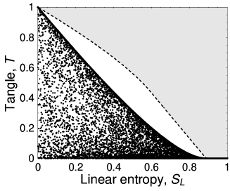
Figure 2: Numerical simulation from our phenomenological model qualitatively reproducing the behavior of a dichroic scattering system. The gray region represents unphysical states and it is bounded from below by MEMS (dashed curve). The lower continuous thick curve represents Werner states.

The numerical simulation shows that a local dichroic scatterer may generate sub-Werner two-qubit states, that is states located below the Werner curve in the tangle-linear entropy plane. The qualitative agreement between the result of this simulation and the experimental findings shown in Fig. 3 of Ref. Pue is evident.

V.1.1 Discussion

It should be noticed that while we used the equality symbol in writing Eq. (50), we had to use the proportionality symbol in writing Eq. (51). This is a consequence of the Hermitean character of the Jones matrix $T_{H}$ that generates a non-trace-preserving map. In fact, in this case from $M=M_{D}M_{\Delta}(p)$, where $M_{D}=(VT_{H}\otimes T_{H}^{*}V^{\dagger})/2$ and $M_{\Delta}(p)=[V\mathcal{M}_{\Delta}(p)V^{\dagger}]/2$ [see Eq. (12)], we obtain $\mathrm{Tr}(\widetilde{\rho}_{\mathcal{E}})=(d_{0}^{2}+d_{1}^{2})/2\neq 1$. Moreover, Eq. (37) gives

$$\begin{array}[]{rcl}{\rho}_{\mathcal{E}}^{B}&=&\displaystyle{\mathrm{Tr}|_{A}({\rho}_{\mathcal{E}})}\\ \\ &=&\displaystyle{\frac{X_{0}}{2}-p\left(\frac{d_{0}^{2}-d_{1}^{2}}{d_{0}^{2}+d_{1}^{2}}\right)\frac{X_{1}\sin 2\theta+X_{3}\cos 2\theta}{2}},\end{array}$$ (55)

where ${\rho}_{\mathcal{E}}=\widetilde{\rho}_{\mathcal{E}}/\mathrm{Tr}(\widetilde{\rho}_{\mathcal{E}})$. This result is in contradiction, for $d_{0}\neq d_{1}$, with the locality constraint expressed by Eq. (26) which requires

$$\rho_{\mathcal{E}}^{B}=\frac{X_{0}}{2}.$$ (56)

As we already discussed in the previous Section, only the latter result seems to be physically meaningful since photons in path $B$, described by $\rho_{\mathcal{E}}^{B}$, cannot carry information about device $\mathcal{T}_{A}$ which is located across path $A$. On the contrary, Eq. (55) shows that $\rho_{\mathcal{E}}^{B}$ is expressed in terms of the four physical parameters $p,d_{0},d_{1}$ and $\theta$ that characterize $\mathcal{T}_{A}$. Is there a contradiction here?

In fact, there is none! One should keep in mind that Eq. (55) expresses the one-qubit reduced density matrix $\rho_{\mathcal{E}}^{B}$ that is extracted from the two-qubit density matrix $\rho_{\mathcal{E}}$ after the latter has been reconstructed by the two observers Alice and Bob by means of nonlocal coincidence measurements. Such matrix contains information about both qubits and, therefore, contains also information about $\mathcal{T}_{A}$. Conversely, $\rho^{B}_{\mathcal{E}}=X_{0}/2$ in Eq. (56), is the reduced density matrix that could be reconstructed by Bob alone via local measurements before he and Alice had compared their own experimental results and had selected from the raw data the coincidence counts.

From a physical point of view, the discrepancy between Eq. (55) and Eq. (56) is due to the polarization-dependent losses (that is, $d_{0}\neq d_{1}$) that characterize dichroic optical devices and it is unavoidable when such elements are present in an experimental setup. Actually, it has been already noticed that a dichroic optical element necessarily performs a kind of post-selective measurement Brunner et al. (2003). In our case coincidence measurements post-select only those photons that have not been absorbed by the dichroic elements present in the setup. However, since in any SPDC setup even the initial singlet state is actually a post-selected state (in order to cut off the otherwise overwhelming vacuum contribution), the practical use of dichroic devices does not represent a severe limitation for such setups.

V.2 Example 2: Generation of two-qubit MEMS states

In the previous subsection we have shown that it is possible to generate two-qubit states represented by points upon and below the Werner curve in the tangle-linear entropy plane, by operating on a single qubit (local operations) belonging to a pair initially prepared in the entangled singlet state. In another paper Aie (b) we have shown that it is also possible to generate MEMS states (see, e.g., Peters et al. (2004); Barbieri et al. (2004) and references therein), via local operations. However, the price to pay in that case was the necessity to use a dichroic device that could not be represented by a “physical”, namely a trace-preserving, quantum map. In the present subsection, as an example illustrating the usefulness of our conceptual scheme, we show that by allowing bi-local operations performed by two separate optical devices $\mathcal{T}_{A}$ and $\mathcal{T}_{B}$ located as in Fig. 1, it is possible to achieve MEMS states without using dichroic devices.

To this end, let us start by rewriting explicitly Eq. (30), where the most general bi-local quantum map $\mathcal{E}[\rho]=\mathcal{E}_{A}\otimes\mathcal{E}_{B}[\rho]$ operating upon the generic input two-qubit state $\rho$, is represented by a Kraus decomposition:

$$\rho_{\mathcal{E}}=\mathcal{E}_{A}\otimes\mathcal{E}_{B}[\rho]=\sum_{\mu,\nu}\lambda_{\mu}\lambda_{\nu}\bigl{(}A_{\mu}\otimes B_{\nu}\bigr{)}\,\rho\,\bigl{(}A_{\mu}^{\dagger}\otimes B_{\nu}^{\dagger}\bigr{)},$$ (57)

where now the equality symbol can be used since we assume that both single-qubit maps $\mathcal{E}_{A}$ and $\mathcal{E}_{B}$ are trace-preserving,

$$\sum_{\mu=0}^{3}\lambda_{\mu}A_{\mu}^{\dagger}A_{\mu}=I=\sum_{\nu=0}^{3}\lambda_{\nu}B_{\nu}^{\dagger}B_{\nu},$$ (58)

but not necessarily unital: $\mathcal{E}_{F}[I]\neq I,\,F\in\{A,B\}$ Ziman and Bužek (2005). Under the action of $\mathcal{E}$, the initial state of each qubit travelling in path $A$ or path $B$ is transformed into either the output state

$$\rho_{\mathcal{E}}^{A}=\mathrm{Tr}|_{B}(\rho_{\mathcal{E}})=\sum_{\mu=0}^{3}\lambda_{\mu}A_{\mu}\rho^{A}A_{\mu}^{\dagger},$$ (59)

or

$$\rho_{\mathcal{E}}^{B}=\mathrm{Tr}|_{A}(\rho_{\mathcal{E}})=\sum_{\nu=0}^{3}\lambda_{\nu}B_{\nu}\rho^{B}B_{\nu}^{\dagger},$$ (60)

respectively, where $\rho^{A}=\mathrm{Tr}|_{B}(\rho)$, and $\rho^{B}=\mathrm{Tr}|_{A}(\rho)$. Without loss of generality, we assume that the two qubits are initially prepared in the singlet state: $\rho=\rho_{s}$. Then Eqs. (59-60) reduce to $\rho_{\mathcal{E}}^{F}=\sum_{\alpha}F_{\alpha}F_{\alpha}^{\dagger}/2,\;F\in\{A,B\}$. From the previous analysis [see Eqs. (30-32)] we know that to each bi-local quantum map $\mathcal{E}_{A}\otimes\mathcal{E}_{B}$ can be associated a pair of classical Mueller matrices $\mathcal{M}_{A}$ and $\mathcal{M}_{B}$ such that

$$(\rho_{\mathcal{E}}^{R})_{\alpha\beta}=\sum_{\mu,\nu}\left(\mathcal{M}^{A}\otimes\mathcal{M}^{B}\right)_{\alpha\beta,\mu\nu}(\rho_{s}^{R})_{\mu\nu}.$$ (61)

The real-valued Mueller matrices $M_{A}$ and $M_{B}$ associated via Eq. (12) to $\mathcal{M}_{A}$ and $\mathcal{M}_{B}$, respectively, can be written as

$$M_{A}=\left[\begin{array}[]{cc}1&\mathbf{0}^{T}\\ {\bf a}&A\\ \end{array}\right],\qquad M_{B}=\left[\begin{array}[]{cc}1&\mathbf{0}^{T}\\ {\bf b}&B\\ \end{array}\right],$$ (66)

where Eq. (15) with $\mathbf{d}_{A}=\mathbf{0}=\mathbf{d}_{B}$ and $M_{00}=1$ has been used, and

$$\mathbf{a}=\left[\begin{array}[]{c}a_{1}\\ a_{2}\\ a_{3}\end{array}\right],\qquad\mathbf{b}=\left[\begin{array}[]{c}b_{1}\\ b_{2}\\ b_{3}\end{array}\right],$$ (73)

are the polarizance vectors of $M_{A}$ and $M_{B}$, respectively. We remember that the condition $\mathbf{d}_{A}=\mathbf{d}_{B}=\mathbf{0}$ is a consequence of the fact that both maps $\mathcal{E}_{A}$ and $\mathcal{E}_{B}$ are trace-preserving, while the conditions $\mathbf{a}\neq\mathbf{0}$ and $\mathbf{b}\neq\mathbf{0}$ reflect the non-unital nature of $\mathcal{E}_{A}$ and $\mathcal{E}_{B}$. With this notation we can rewrite Eqs. (59-60) as

$$\rho_{\mathcal{E}}^{A}=\frac{1}{2}\sum_{\mu=0}^{3}a_{\mu}X_{\mu},$$ (74)

$$\rho_{\mathcal{E}}^{B}=\frac{1}{2}\sum_{\nu=0}^{3}b_{\nu}X_{\nu},$$ (75)

where we have defined $a_{0}=1=b_{0}$. Moreover, the output two-qubit density matrix $\rho_{\mathcal{E}}=\mathcal{E}[\rho_{s}]$ can be decomposed into a real and an imaginary part as $\rho_{\mathcal{E}}=\rho_{\mathcal{E}}^{\mathrm{Re}}+i\rho_{\mathcal{E}}^{\mathrm{Im}}$, where

$$\rho_{\mathcal{E}}^{\mathrm{Re}}=\frac{1}{4}\left[\begin{array}[]{cccc}\alpha_{+}^{+}&\beta_{+}&\gamma_{+}&\delta_{+}\\ \beta_{+}&\alpha_{-}^{+}&\delta_{-}&\gamma_{-}\\ \gamma_{+}&\delta_{-}&\alpha_{+}^{-}&\beta_{-}\\ \delta_{+}&\gamma_{-}&\beta_{-}&\alpha_{-}^{-}\end{array}\right],$$ (80)

and

$$\rho_{\mathcal{E}}^{\mathrm{Im}}=\frac{1}{4}\left[\begin{array}[]{cccc}0&-\xi_{+}&-\eta_{+}&-\tau_{+}\\ \xi_{+}&0&-\tau_{-}&-\eta_{-}\\ \eta_{+}&\tau_{-}&0&-\xi_{-}\\ \tau_{+}&\eta_{-}&\xi_{-}&0\end{array}\right],$$ (85)

with

$$\alpha_{\pm}^{+}\equiv(1+a_{3})\pm[b_{3}(1+a_{3})-C_{33}],$$

$$\alpha_{\pm}^{-}\equiv(1-a_{3})\pm[b_{3}(1-a_{3})+C_{33}],$$ (86)

and

$$\beta_{\pm}\equiv b_{1}\pm(a_{3}b_{1}-C_{31}),$$

$$\gamma_{\pm}\equiv a_{1}\pm(a_{1}b_{3}-C_{13}),$$

$$\delta_{\pm}\equiv a_{1}b_{1}-C_{11}\mp(a_{2}b_{2}-C_{22}),$$ (87)

and

$$\xi_{\pm}\equiv b_{2}\pm(a_{3}b_{2}-C_{32}),$$

$$\eta_{\pm}\equiv a_{2}\pm(a_{2}b_{3}-C_{23}),$$

$$\tau_{\pm}\equiv a_{2}b_{1}-C_{21}\pm(a_{1}b_{2}-C_{12}),$$ (88)

where $C_{ij}\equiv(AB^{T})_{ij},\,i,j\in\{1,2,3\}$.

At this point, our goal is to determine the two vectors $\mathbf{a},\,\mathbf{b}$ and the two $3\times 3$ matrices $A,\,B$ such that $\rho_{\mathcal{E}}^{\mathrm{Im}}=0$ and

$$\rho_{\mathcal{E}}^{\mathrm{Re}}=\rho_{\mathrm{MEMS}}=\left[\begin{array}[]{cccc}{g(p)}/{2}&0&0&{p}/{2}\\ 0&1-g(p)&0&0\\ 0&0&0&0\\ {p}/{2}&0&0&{g(p)}/{2}\end{array}\right],$$ (93)

where

$$g(p)=\left\{\begin{array}[]{ccc}{2}/{3}\,,&&0\leq p\leq{2}/{3},\\ \\ p\,,&&{2}/{3}<p\leq 1.\end{array}\right.$$ (97)

To this end, first we calculate $\mathbf{a}$ and $\mathbf{b}$ by imposing:

$$\rho_{\mathcal{E}}^{A}=\rho_{\mathrm{MEMS}}^{A}=\left[\begin{array}[]{cc}1-g(p)/2&0\\ 0&g(p)/2\end{array}\right],$$ (100)

$$\rho_{\mathcal{E}}^{B}=\rho_{\mathrm{MEMS}}^{B}=\left[\begin{array}[]{cc}g(p)/2&0\\ 0&1-g(p)/2\end{array}\right],$$ (103)

respectively. Note that only fulfilling Eqs. (100-103), together with $\rho_{\mathcal{E}}^{\mathrm{Re}}=\rho_{\mathrm{MEMS}}$ and $\rho_{\mathcal{E}}^{\mathrm{Im}}=0$, will ensure the achievement of true MEMS states. It is surprising that in the current literature the importance of this point is neglected. Thus, by solving Eqs. (100-103) we obtain $a_{1}=a_{2}=0$, $a_{3}=1-g(p)$, and $\mathbf{b}=-\mathbf{a}$, where Eqs. (74-75) have been used. Then, after a little of algebra, it is not difficult to find that a possible bi-local map $\mathcal{E}=\mathcal{E}_{A}\otimes\mathcal{E}_{B}$ that generates a solution $\rho_{\mathcal{E}}$ for the equation $\rho_{\mathcal{E}}=\rho_{\mathrm{MEMS}}$, can be expressed as in Eqs. (61-66) in terms of the two real-valued Mueller matrices

$$\begin{array}[]{rcl}M_{A}&=&\left[\begin{array}[]{cccc}1&0&0&0\\ 0&\sqrt{p}&0&0\\ 0&0&\sqrt{p}&0\\ 1-g(p)&0&0&g(p)\end{array}\right],\\ \\ M_{B}&=&\left[\begin{array}[]{cccc}1&0&0&0\\ 0&-\sqrt{p}&0&0\\ 0&0&\sqrt{p}&0\\ g(p)-1&0&0&-g(p)\end{array}\right].\end{array}$$ (104)

It is easy to check that both $M_{A}$ and $M_{B}$ are physically admissible Mueller matrices since the associated matrices $H_{A}$ and $H_{B}$ have the same spectrum made of non-negative eigenvalues $\{\lambda_{\mu}\}=\{\lambda_{0},\,\lambda_{1},\,\lambda_{2},\,\lambda_{3}\}$. In particular:

$$\{\lambda_{\mu}\}=\left\{0,\,1-p,\,0,\,1+p\right\},\quad\mathrm{for}\quad{2}/{3}<p\leq 1.$$ (105)

and

$$\{\lambda_{\mu}\}=\left\{0,\frac{1}{3},\frac{5-\sqrt{1+36p}}{6},\frac{5+\sqrt{1+36p}}{6}\right\},$$ (106)

for $0\leq p\leq{2}/{3}$. It is also easy to see that the map $\mathcal{E}$ can be decomposed as in Eq. (57) in a Kraus sum with $A_{0}=A_{2}=0$,

$$A_{1}\sqrt{\lambda_{1}}=\left[\begin{array}[]{cc}0&\sqrt{1-p}\\ 0&0\end{array}\right],\quad A_{3}\sqrt{\lambda_{3}}=\left[\begin{array}[]{cc}1&0\\ 0&\sqrt{p}\end{array}\right],$$ (111)

and $B_{0}=B_{2}=0$,

$$B_{1}\sqrt{\lambda_{1}}=\left[\begin{array}[]{cc}0&0\\ 0&\sqrt{1-p}\end{array}\right],\quad B_{3}\sqrt{\lambda_{3}}=\left[\begin{array}[]{cc}0&-\sqrt{p}\\ 1&0\end{array}\right],$$ (116)

for ${2}/{3}<p\leq 1$. Analogously, for $0\leq p\leq{2}/{3}$ we have $A_{0}=0$,

$$A_{1}\sqrt{\lambda_{1}}=\left[\begin{array}[]{cc}0&1/\sqrt{3}\\ 0&0\end{array}\right],$$ (119)

$$A_{2}\sqrt{\lambda_{2}}=\left[\begin{array}[]{cc}-\phi_{-}&0\\ 0&\psi_{+}\end{array}\right],\quad A_{3}\sqrt{\lambda_{3}}=\left[\begin{array}[]{cc}\phi_{+}&0\\ 0&\psi_{-}\end{array}\right],$$ (124)

and $B_{0}=0$,

$$B_{1}\sqrt{\lambda_{1}}=\left[\begin{array}[]{cc}0&0\\ 0&1/\sqrt{3}\end{array}\right],$$ (127)

$$B_{2}\sqrt{\lambda_{2}}=\left[\begin{array}[]{cc}0&\psi_{+}\\ \phi_{-}&0\end{array}\right],\quad B_{3}\sqrt{\lambda_{3}}=\left[\begin{array}[]{cc}0&-\psi_{-}\\ \phi_{+}&0\end{array}\right],$$ (132)

where

$$\phi_{\pm}\equiv\sqrt{\frac{1}{2}\left(1\pm\frac{1+6p}{\sqrt{1+36p}}\right)},$$ (133)

(134)

$$\psi_{\pm}\equiv\sqrt{\frac{1}{3}\left(1\pm\frac{1-9p}{\sqrt{1+36p}}\right)}.$$

Note that these coefficients satisfy the following relations:

$$\sum_{\mu=0}^{3}\lambda_{\mu}A_{\mu}^{\dagger}A_{\mu}=\phi_{+}^{2}+\phi_{-}^{2}=1,$$ (135)

$$\sum_{\nu=0}^{3}\lambda_{\nu}B_{\nu}^{\dagger}B_{\nu}=\frac{1}{3}+\psi_{+}^{2}+\psi_{-}^{2}=1.$$ (136)

A straightforward calculation shows that the single-qubit maps $\mathcal{E}_{A}$ and $\mathcal{E}_{B}$ are trace-preserving but not unital, since

$$\sum_{\mu=0}^{3}\lambda_{\mu}A_{\mu}A_{\mu}^{\dagger}=\left[\begin{array}[]{cc}2-g(p)&0\\ 0&g(p)\end{array}\right],$$ (139)

and

$$\sum_{\nu=0}^{3}\lambda_{\nu}B_{\nu}B_{\nu}^{\dagger}=\left[\begin{array}[]{cc}g(p)&0\\ 0&2-g(p)\end{array}\right].$$ (142)

At this point our task has been fully accomplished. However, before concluding this subsection, we want to point out that both maps $\mathcal{E}_{A}$ and $\mathcal{E}_{B}$ must depend on the same parameter $p$ in order to generate proper MEMS states. This means that either a classical communication must be established between $\mathcal{T}_{A}$ and $\mathcal{T}_{B}$ in order to fix the same value of $p$ for both devices, or a classical signal encoding the information about the value of $p$ must be sent towards both $\mathcal{T}_{A}$ and $\mathcal{T}_{B}$.

V.2.1 Physical implementation

Now we furnish a straightforward physical implementation for the quantum maps presented above. Up to now, several linear optical schemes generating MEMS states were proposed and experimentally tested. Kwiat and coworkers Peters et al. (2004) were the first to achieve MEMS using photon pairs from spontaneous parametric down conversion. Basically, they induced decoherence in SPDC pairs initially prepared in a pure entangled state by coupling polarization and frequency degrees of freedom of the photons. At the same time, a somewhat different scheme was used by De Martini and coworkers Barbieri et al. (2004) who instead used the spatial degrees of freedom of SPDC photons to induce decoherence. In such a scheme the use of spatial degrees of freedom of photons required the manipulation of not only the emitted SPDC photons, but also of the pump beam.

In this subsection, we show that both single-qubit maps $\mathcal{E}_{A}$ and $\mathcal{E}_{B}$ can be physically implemented as linear optical networks Skaar et al. (2004) where polarization and spatial modes of photons are suitably coupled, without acting upon the pump beam. The basic building blocks of such networks are polarizing beam splitters (PBSs), half-waveplates (HWPs), and mirrors. Let $|i,N\rangle$ be a single-photon basis, where the indices $i$ and $N$ label polarization and spatial modes of the electromagnetic field, respectively. We can also write $|i,N\rangle=\hat{a}_{iN}^{\dagger}|0\rangle$ in terms of the annihilation operators $\hat{a}_{iN}$ and the vacuum state $|0\rangle$. A polarizing beam splitter distributes horizontal ($i=H$) and vertical ($i=V$) polarization modes over two distinct spatial modes, say $N=n$ and $N=m$, as follows:

$$\begin{array}[]{lcl}|H,n\rangle_{\mathrm{in}}\rightarrow|H,n\rangle_{\mathrm{out}}&\mathrm{and}&|V,n\rangle_{\mathrm{in}}\rightarrow|V,m\rangle_{\mathrm{out}},\\ \\ |H,m\rangle_{\mathrm{in}}\rightarrow|H,m\rangle_{\mathrm{out}}&\mathrm{and}&|V,m\rangle_{\mathrm{in}}\rightarrow|V,n\rangle_{\mathrm{out}},\end{array}$$ (143)

as illustrated in Fig. 3.

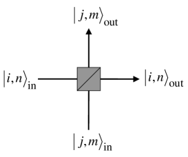
Figure 3: The polarizing beam splitter couples horizontal and vertical polarization modes ($i,j\in\{H,V\}$), with two distinct spatial modes $N=n$ and $N=m$ of the electromagnetic field.

A half-waveplate does not couple polarization and spatial modes of the electromagnetic field and can be represented by a $2\times 2$ Jones matrix $T_{HWP}(\theta)$ as

$$T_{HWP}(\theta)=\left[\begin{array}[]{cc}-\cos 2\theta&-\sin 2\theta\\ -\sin 2\theta&\cos 2\theta\end{array}\right],$$ (144)

where $\theta$ is the angle the optic axis makes with the horizontal polarization. Two half-waveplates in series constitute a polarization rotator represented by $T_{R}(\theta)=T_{HWP}(\theta_{0}+{\theta}/{2})T_{HWP}(\theta_{0})$, where $\theta_{0}$ is an arbitrary angle and

$$T_{R}(\theta)=\left[\begin{array}[]{cc}\cos\theta&-\sin\theta\\ \sin\theta&\cos\theta\end{array}\right].$$ (145)

By combining these basic elements, composite devices may be built. Figures 4 (a-b) show the structure of a horizontal (a), and vertical (b) variable beam splitter, denoted HVBS and VVBS, respectively. HVBS performs the following transformation

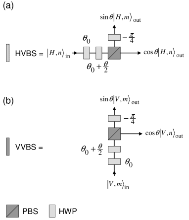
Figure 4: The variable beam splitters HVBS and VVBS.

$$|H,n\rangle_{\mathrm{in}}\rightarrow\cos\theta|H,n\rangle_{\mathrm{out}}+\sin\theta|H,m\rangle_{\mathrm{out}},$$ (146)

while VVBS makes

$$|V,m\rangle_{\mathrm{in}}\rightarrow\cos\theta|V,n\rangle_{\mathrm{out}}+\sin\theta|V,m\rangle_{\mathrm{out}}.$$ (147)

At this point we have all the ingredients necessary to built the optical linear networks corresponding to our maps. We begin by illustrating in detail the optical network implementing $\mathcal{E}_{A}$ (for $2/3<p\leq 1$), which is shown in Fig. 5.

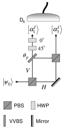
Figure 5: Linear optical network implementing $\mathcal{E}_{A}$ (for $2/3<p\leq 1$), for MEMS I generation.

Let $|\psi_{0}\rangle=a|H\rangle+b|V\rangle$ be the input single-photon state entering the network. If we define the VVBS angle

$$\theta_{p}=\arccos\sqrt{p},$$ (148)

then it is easy to obtain after a straightforward calculation:

$$|\alpha_{1}^{I}\rangle=\sqrt{\lambda_{1}}A_{1}|\psi_{0}\rangle=b\,\sqrt{1-p}\,|H\rangle,$$ (149)

$$|\alpha_{3}^{I}\rangle=\sqrt{\lambda_{3}}A_{3}|\psi_{0}\rangle=a|H\rangle+b\,\sqrt{p}\,|V\rangle.$$ (150)

Since detector $\mathbf{\textsf{D}}_{\mathbf{\textsf{A}}}$ does not distinguish spatial mode $1$ from spatial mode $2$, the two states $|\alpha_{1}^{I}\rangle$ and $|\alpha_{3}^{I}\rangle$, sum incoherently and the single-photon output density matrix can be written as $\rho_{\mathcal{E}_{A}}=|\alpha_{1}^{I}\rangle\langle\alpha_{1}^{I}|+|\alpha_{3}^{I}\rangle\langle\alpha_{3}^{I}|$, where

$$\rho_{\mathcal{E}_{A}}=\left[\begin{array}[]{cc}|a|^{2}+|b|^{2}(1-p)&ab^{*}\sqrt{p}\\ a^{*}b\sqrt{p}&p|b|^{2}\end{array}\right].$$ (153)

Of course, if we write the input density matrix as $\rho_{0}=|\psi_{0}\rangle\langle\psi_{0}|$, it is easy to see that

$$\rho_{\mathcal{E}_{A}}=\sum_{\mu=0}^{3}\lambda_{\mu}A_{\mu}\rho_{0}A_{\mu}^{\dagger}.$$ (154)

where Eqs. (111) have been used. Equation (154), together with Eq. (59), proves the equivalence between the quantum map $\mathcal{E}_{A}$ and the linear optical setup shown in Fig. 5. Note that the Mach-Zehnder interferometers present in Figs. 5 and 6 are balanced, that is their arms have the same optical length. In a similar manner, we can physically implement $\mathcal{E}_{B}$ (for $2/3<p\leq 1$), in the optical network shown in Fig. 6, where we have defined

$$|\beta_{1}^{I}\rangle=\sqrt{\lambda_{1}}B_{1}|\psi_{0}\rangle=b\,\sqrt{1-p}\,|V\rangle,$$ (155)

$$|\beta_{3}^{I}\rangle=\sqrt{\lambda_{3}}B_{3}|\psi_{0}\rangle=-b\,\sqrt{p}\,|H\rangle+a\,|V\rangle,$$ (156)

and, again, $\rho_{\mathcal{E}_{B}}=|\beta_{1}^{I}\rangle\langle\beta_{1}^{I}|+|\beta_{3}^{I}\rangle\langle\beta_{3}^{I}|$.

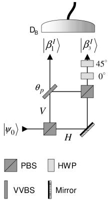
Figure 6: Linear optical network implementing $\mathcal{E}_{B}$ (for $2/3<p\leq 1$), for MEMS I generation.

The optical networks necessary to realize quantum maps generating MEMS II states are a bit more complicated. In order to illustrate them we need to define the following two angles $\theta_{1/3}$ and $\theta_{\psi}$ that determine the transmission amplitudes of two VVBSs used in the MEMS II networks:

$$\theta_{1/3}=\arccos\sqrt{\frac{1}{3}},$$ (157)

$$\theta_{\psi}=\arccos\left(\sqrt{\frac{3}{2}}\;\psi_{+}\right).$$ (158)

In addition, a third angle $\theta_{\phi}$ determining the transmission amplitudes of a HVBS, must be introduced:

$$\theta_{\phi}=\arccos\phi_{+}.$$ (159)

Then, the map $\mathcal{E}_{A}$ (for $0\leq p\leq 2/3$), is realized by the optical network shown in Fig. 7, where we have defined

$$|\alpha_{2}^{II}\rangle=\sqrt{\lambda_{2}}A_{2}|\psi_{0}\rangle=-a\,\phi_{-}\,|H\rangle+b\,\psi_{+}\,|V\rangle,$$ (160)

$$|\alpha_{3}^{II}\rangle=\sqrt{\lambda_{3}}A_{3}|\psi_{0}\rangle=a\,\phi_{+}\,|H\rangle+b\,\psi_{-}\,|V\rangle,$$ (161)

$$|\alpha_{1}^{II}\rangle=\sqrt{\lambda_{1}}A_{1}|\psi_{0}\rangle=\frac{b}{\sqrt{3}}|H\rangle.$$ (162)

In this case, incoherent detection produces the output mixed state $\rho_{\mathcal{E}_{A}}=|\alpha_{2}^{II}\rangle\langle\alpha_{2}^{II}|+|\alpha_{3}^{II}\rangle\langle\alpha_{3}^{II}|+|\alpha_{1}^{II}\rangle\langle\alpha_{1}^{II}|$.

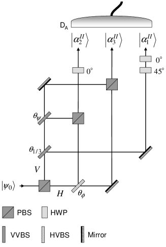
Figure 7: Linear optical network implementing $\mathcal{E}_{A}$ (for $0\leq p\leq 2/3$), for MEMS II generation. Each of the two Mach-Zehnder interferometers constituting the network are balanced.

Finally, the map $\mathcal{E}_{B}$ (for $0\leq p\leq 2/3$), is realized by the optical network shown in Fig. 8, where we have defined

$$|\beta_{2}^{II}\rangle=\sqrt{\lambda_{2}}B_{2}|\psi_{0}\rangle=b\,\psi_{+}\,|H\rangle+a\,\phi_{-}\,|V\rangle,$$ (163)

$$|\beta_{3}^{II}\rangle=\sqrt{\lambda_{3}}B_{3}|\psi_{0}\rangle=-b\,\psi_{-}\,|H\rangle+a\,\phi_{+}\,|V\rangle,$$ (164)

$$|\beta_{1}^{II}\rangle=\sqrt{\lambda_{1}}B_{1}|\psi_{0}\rangle=\frac{b}{\sqrt{3}}|V\rangle.$$ (165)

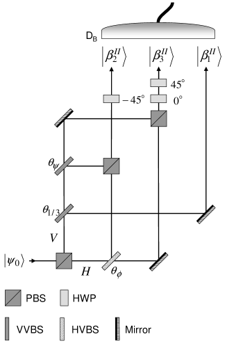
Figure 8: Linear optical network implementing $\mathcal{E}_{B}$ (for $0\leq p\leq 2/3$), for MEMS II generation. Each of the two Mach-Zehnder interferometers constituting the network are balanced.

As before, now we have $\rho_{\mathcal{E}_{B}}=|\beta_{2}^{II}\rangle\langle\beta_{2}^{II}|+|\beta_{3}^{II}\rangle\langle\beta_{3}^{II}|+|\beta_{1}^{II}\rangle\langle\beta_{1}^{II}|$.

VI Summary and conclusions

Classical polarization optics and quantum mechanics of two-level systems are two different branches of physics that share the same mathematical machinery. In this paper we have described the analogies and connections between these two subjects. In particular, after a review of the matrix formalism of classical polarization optics, we established the exact relation between one- and two-qubit quantum maps and classical description of linear optical processes. Finally, we successfully applied the formalism just developed, to two cases of practical utility.

We believe that the present paper will be useful to both the classical and the quantum optics community since it enlightens and puts on a rigorous basis, the so-widely used relations between classical polarization optics and quantum mechanics of qubits. A particularly interesting aspect of our work is that we describe in detail how dichroic devices (i.e., devices with polarization-dependent losses), fit into this general scheme.