Quantum dynamics of bound entangled states

Abstract

By using the partial transpose and realignment method,we study the time evolution of the bound entanglement under the bilinear-biquadratic Hamiltonian. For the initial Horodecki’s bound entangled state, it keeps bound entangled for some time, while for the initial bound entangled states constructed from the unextendable product basis, they become free once the time evolution begins. The time evolution provides a new way to construct bound entangled states, and also gives a method to free bound entanglement.

Quantum information theory has drawn much attention in the last decade, and in the quantum information theory, quantum entanglement plays an important role as it can be utilized to realize some quantum processes nielsen . In realistic world, due to the interaction between the system and the environment, most states in nature are mixed and the set of mixed states is dense in Hilbert space. The mixed entangled states can be divided into two classes horodecki , one is free, which means that the state can be distilled, the other is bound, which means that the state cannot be distilled. The bound entangled state is thought to be useless in quantum communication. However, the bound entangled state (BES) can produce a nonclassical effect, which is called activation of bound entanglement. The underlying concept originates from a formal entanglement-energy analogy en-en ; acta ; rohrlich . It implies that the bound entanglement is like the energy of a system confined in a shallow potential well. If we add a small amount of extra energy to the system, its energy can be deliberated. One of the main consequence of the existence of BESs is that it reveals a transparent form of irreversibility in entanglement processing review . The irreversibility can be viewed as an analog to irreversible thermodynamics processes thermal .

The bound entanglement can possibly get free if we add some energy to it. In this paper, we see what happens if we let the BES undergoes some quantum dynamical evolution under physical Hamiltonians. We will see that BESs can be free via time evolution. The time-evolved BES can be also considered as the original BES with an extra time parameter $t$, and this provides a way to construct more general BESs.

There are some measures to detect entangled state in high-dimensional Hilbert space. For example, Peres-Horodecki criterion based on partial transpose (PT) PPT1 ; PPT2 ; negativity and the realignment criterion realign1 ; realign2 . Consider a density matrix $\rho$ in a $n\otimes n$ system , the PT with respect to the second system, and the realignment of the density matrix is given by $(\rho^{T_{2}})_{ij,kl}=\rho_{il,kj}$ $(\rho^{R})_{ij,kl}=\rho_{ik,jl}$ , respectively. Two quantities are defined as

$$N_{1}=\frac{\parallel\rho^{T_{2}}\parallel-1}{2},\;N_{2}=\frac{\parallel\rho^{R}\parallel-1}{2},$$ (1)

where the first is the negativity negativity . The trace norm $\parallel A\parallel$ is given by $\parallel A\parallel=$tr$\sqrt{AA^{\dagger}}$. Either $N_{1}>0$ or $N_{2}>0$ indicates that the state is entangled, $N_{1}=0$ and $N_{2}>0$ indicates that the state is bound entangled, and $N_{1}>0$ means that the state is free entangled Simon .

To study time evolution,  we should have a suitable Hamiltonian. We will concentrate on $3\otimes 3$ system in this study, and without loss of generality, regard this system as a two spin-one system. The most representative interacting model in spin-one system is the bilinear-biquadratic model affleck . The corresponding Hamiltonian is given by affleck .

$$H=\mathbf{s}_{1}\cdot\mathbf{s}_{2}-\beta(\mathbf{s}_{1}\cdot\mathbf{s}_{2})^{2}.$$ (2)

Here, $\mathbf{s}_{i}\$denotes the spin-1 operator. As we know, for spin-1 system, the swapping operator $\mathbf{S}_{12}$ can be written as xgwang

$$\mathbf{S}_{12}=(\mathbf{s}_{1}\cdot\mathbf{s}_{2})^{2}+\mathbf{s}_{1}\cdot\mathbf{s}_{2}-1,$$ (3)

which is invariant under the $SU(3)$ unitary transformation. The singlet projection operator is written as

$$\mathbf{P}_{12}=\frac{1}{3}\left[(\mathbf{s}_{1}\cdot\mathbf{s}_{2})^{2}-1\right].$$ (4)

Then, the Hamiltonian can be rewritten in terms of swapping operator and projective operator,

$$H=\mathbf{S}_{12}-3(1+\beta)\mathbf{P}_{12}-\beta.$$ (5)

It is obvious that swapping operator and projective operator are commutative, so that the unitary matrix $U(t)$ can be obtained as

$$U(t)=e^{-iHt}=e^{-it\mathbf{S}_{12}}e^{i3(1+\beta)t\mathbf{P}_{12}}e^{it\beta}.$$ (6)

We have $\mathbf{S}_{12}^{2}=1$ and $\mathbf{P}_{12}^{2}=\mathbf{P}_{12}$, then

$$e^{-it\mathbf{S}_{12}} = \cos t-i\sin t\mathbf{S}_{12},$$

$$e^{i3(1+\beta)t\mathbf{P}_{12}} = 1+(e^{i3(1+\beta)t}-1)\mathbf{P}_{12}.$$ (7)

In this way, we can get the evolution operator exactly.

For clarity, we consider the case of $\beta=-1$. The Hamiltonian can be reduced to the swap

$$H=\mathbf{S}=\mathbf{S}_{12}$$ (8)

up to a additive constant. In the following, we will study the time-evolution of bound entangled state govenered by the Hamiltonian. The initial state will evolve under the unitary density matrix

$$U(t)=e^{-itH}=\cos t-i\sin t\mathbf{S}.$$ (9)

At time $t$, the density matrix $\rho(t)=e^{-itH}\rho(0)e^{itH}$.

The two-spin BES we are considering, described by Horodecki in Ref. horodecki , is given by

$$\rho_{\alpha}(0)=\frac{2}{7}\mathbf{P}_{+}+\frac{\alpha}{7}\varrho_{+}+\frac{5-\alpha}{7}\varrho_{-},\ 2\leq\alpha\leq 5,$$ (10)

where

$$\mathbf{P}_{+} = |\Psi_{+}\rangle\langle\Psi_{+}|,|\Psi_{+}\rangle=\frac{1}{\sqrt{3}}(|00\rangle+|11\rangle+|22\rangle),$$

$$\varrho_{+} = \frac{1}{3}(|01\rangle\langle 01|+|12\rangle\langle 12|+|20\rangle\langle 20|),$$

$$\varrho_{-} = \frac{1}{3}(|10\rangle\langle 10|+|21\rangle\langle 21|+|02\rangle\langle 02|)=\mathbf{S}\varrho_{+}\mathbf{S}.$$

In Ref. horodecki , Horodecki have demonstrated that

$$\rho_{\alpha}\text{ is }\left\{\begin{array}[]{l}\text{separable for }2\leq\alpha\leq 3\\ \text{bound entangled for }3<\alpha\leq 4,\\ \text{free entangled for }\alpha<4\leq 5.\end{array}\right.$$

An interesting feature of this state is that it is invariant under the joint transformation of exchange $\alpha\leftrightarrow 5-\alpha$ and swap of two particles. It is clear that the density matrix $\rho_{\alpha}$ has four distinct eigenvalues, which are $2/7$, $0$, $(5-\alpha)/21$, $\alpha/21$. They are non-degenerate, 2-fold degenerate, 3-fold degenerate, and 3-fold degenerate, respectively.

From the expression of the state, after PT, the trace norm of the partially transposed state is given by

$$\left\|\rho_{\alpha}^{T_{2}}\right\| = \frac{1}{7}\Big{[}2+\frac{1}{2}(5+\sqrt{41-4\alpha(5-\alpha)}$$

$$+\left|5-\sqrt{41-4\alpha(5-\alpha)}\right|)\Big{]}\text{ }$$

$$= \text{ }\left\{\begin{array}[]{l}1\text{ for }2\leq\alpha\leq 4,\\ \frac{1}{7}\left(2+\sqrt{41-4\alpha(5-\alpha)}\right)\text{ for }\alpha<4\leq 5.\end{array}\right.$$

Note that the realignment in the realignment criteria is equivalent to a one-side swap followed by a PT Fan , namely, $\left\|\rho_{\alpha}^{R}\right\|=\left\|\left(S\rho_{\alpha}\right)^{T_{2}}\right\|.$ It is direct to show that

$$S\rho_{\alpha}=\frac{2}{7}\mathbf{P}_{+}+\frac{\alpha}{7}\mathbf{S}\varrho_{+}+\frac{5-\alpha}{7}\varrho_{+}\mathbf{S}.\$$

Then, after PT, we have

$$\left\|\rho_{\alpha}^{R}\right\|=\frac{1}{21}\left(19+2\sqrt{19-3\alpha(5-\alpha)}\right).$$

From the expression of the two trace norms, an observation is that the exchange $\alpha\longleftrightarrow(5-\alpha)$ does not change the values of the two trace norms.

Now we consider the time evolution of state $\rho_{\alpha}.$ From the evolution operator (9) and the initial state (10), the state at time $t$ is obtained as

$$\rho_{\alpha}(t) = \frac{1}{7}\{2\mathbf{P}_{+}+a(t)\varrho_{+}+b(t)\varrho_{-}+ic(t)[\mathbf{S},\varrho_{-}]\},$$ (12)

$$a(t) = \alpha\cos^{2}t+(5-\alpha)\sin^{2}t$$

$$b(t) = \alpha\sin^{2}t+(5-\alpha)\cos^{2}t\$$

$$c(t) = \sin t\cos t(2\alpha-5)=1/2\sin(2t)(2\alpha-5)$$ (13)

In the derivation of the above equation, we have used the identity $[\mathbf{S},\varrho_{-}]=[\varrho_{+},\mathbf{S}].$ It is obvious that

$$a+b=5,a-b=(2\alpha-5)\cos(2t),$$ (14)

which will be used later.

Let’s study the case in which $t=\pi/2$. At this moment,

$$U(t=\pi/2)=-i\mathbf{S}.$$ (15)

So the density matrix becomes

$$\rho_{\alpha}(\pi/2) = U(\pi/2)\rho_{\alpha}U^{\dagger}(\pi/2)$$ (16)

$$= \frac{2}{7}\mathbf{P}_{+}+\frac{\alpha}{7}\varrho_{-}+\frac{5-\alpha}{7}\varrho_{+}.\$$

The above state can be obtained from $\rho_{\alpha}(0)$ by just exchange $\alpha\longleftrightarrow(5-\alpha).$ But the exchange does not affect the values of trace norms. Thus, the trace norms at time $t=\pi/2$ are the same as those at time $t=0$.

The negativity can be calculated by first making the PT, and diagonalizing the partially transposed density matrix. Making use of the following properties,

$$\mathbf{P}_{+}^{T_{2}} = \frac{\mathbf{S}}{3},\varrho_{\pm}^{T_{2}}=\varrho_{\pm},$$

$$(\mathbf{S}\rho_{-})^{T_{2}} = \frac{1}{3}\left(|00\rangle\langle 11|+|11\rangle\langle 22|+|22\rangle\langle 00|\right)$$

$$(\rho_{-}S)^{T_{2}} = \frac{1}{3}\left(|11\rangle\langle 00|+|22\rangle\langle 11|+|00\rangle\langle 22|\right),$$ (17)

we have

$$\rho_{\alpha}^{T_{2}}(t) = \frac{1}{21}\{2\mathbf{S}+3a(t)\varrho_{+}+3b(t)\varrho_{-}$$ (19)

$$+ic(t)\left(|00\rangle\langle 11|+|11\rangle\langle 22|+|22\rangle\langle 00|\right)$$

$$-ic(t)\left(|11\rangle\langle 00|+|22\rangle\langle 11|+|00\rangle\langle 22|\right)\}.\ \$$

In the basis spanned by $\{|00\rangle,|11\rangle,|22\rangle,|01\rangle,|10\rangle,|12\rangle,|21\rangle,|20\rangle,|02\rangle\},$ matrix $\rho_{\alpha}^{T_{2}}(t)$ can be written in a block-diagonal form

$$\rho_{\alpha}^{T_{2}}(t)=\frac{1}{21}\left(A_{{}_{3\times 3}}\oplus B_{2\times 2}\oplus B_{2\times 2}\oplus B_{2\times 2}\right),$$

$$A_{{}_{3\times 3}}=\left(\begin{array}[]{ccc}2&ic(t)&-ic(t)\\ -ic(t)&2&ic(t)\\ ic(t)&-ic(t)&2\end{array}\right),B_{2\times 2}=\left(\begin{array}[]{cc}a(t)&2\\ 2&b(t)\end{array}\right),$$

where we have used the fact that in this basis, the swap can be written as

$$\mathbf{S}=I_{3\times 3}\oplus\sigma_{x}\oplus\sigma_{x}\oplus\sigma_{x}.$$

and $I_{{}_{3\times 3}}$ is a 3$\times 3$ identity matrix, and $\sigma_{x}$ is the $x$ component of the Pauli matrix vector.

Having the block-diagonal form of $\rho^{T_{2}}(t),$one can obtain the eigenvalues of the partial transposed density matrix, and only the two following eigenvalues are possibly negative

$$\lambda_{1} = \frac{1}{21}\left(2-\sqrt{3}c\right)$$

$$= \frac{1}{42}\left(4-\sqrt{3}|\sin(2t)(2\alpha-5)|\right).$$

$$\lambda_{2} = \frac{1}{42}(a(t)+b(t)-\sqrt{[a(t)-b(t)]^{2}+16})$$ (21)

$$= \frac{1}{42}\left(5-\sqrt{16+(2\alpha-5)^{2}\cos^{2}2t}\right),$$

So, the negativity of $\rho_{\alpha}(t)$ is given by

$$N_{1}=\max(0,-\lambda_{1})+3\max(0,-\lambda_{2}).$$ (22)

Having known analytical expression of $N_{1},$ we next consider the quantity $N_{2}.$ First, we need to obtain matrix $(S\rho_{\alpha}(t))^{T_{2}}.$ From the definition of the BES, we have

$$\mathbf{S}\rho_{\alpha}(t)=\frac{1}{7}\{2\mathbf{P}_{+}+a(t)\mathbf{S}\varrho_{+}+b(t)\mathbf{S}\varrho_{-}+ic(t)\left(\varrho_{-}-\varrho_{+}\right)\}.\$$

After PT, we obtain

$$(S\rho_{\alpha}(t))^{T_{2}} = \frac{1}{21}\{2\mathbf{S}+i3c(t)\left(\varrho_{-}-\varrho_{+}\right)$$

$$+a(t)\left(|11\rangle\langle 00|+|22\rangle\langle 11|+|00\rangle\langle 22|\right)$$

$$+b(t)\left(|00\rangle\langle 11|+|11\rangle\langle 22|+|22\rangle\langle 00|\right)\},\$$

where Eq. (17) is used. In the basis given above, the matrix $(S\rho_{\alpha}(t))^{T_{2}}$ can be written as

$$(S\rho_{\alpha}(t))^{T_{2}}=\frac{1}{21}\left(C_{{}_{3\times 3}}\oplus D_{2\times 2}\oplus D_{2\times 2}\oplus D_{2\times 2}\right),$$

$$C_{{}_{3\times 3}}=\left(\begin{array}[]{ccc}2&b(t)&a(t)\\ a(t)&2&b(t)\\ b(t)&a(t)&2\end{array}\right),D_{2\times 2}=\left(\begin{array}[]{cc}-ic(t)&2\\ 2&ic(t)\end{array}\right)$$

Again, it is of block-diagonal form. The square roots of eigenvalues of $CC^{\dagger}$ are given by

$$\xi_{1} = 2+a+b=7,$$

$$\xi_{2} = \xi_{3}=\sqrt{\left(2-\frac{a+b}{2}\right)^{2}+\frac{3}{4}(a-b)^{2}}$$ (24)

$$= \frac{1}{2}\sqrt{1+3(2\alpha-5)^{2}\cos^{2}(2t)},$$

and the square roots of eigenvalues of $DD^{\dagger}$ are

$$\zeta_{1} = |2+c|=\frac{1}{2}|4+\sin(2t)(2\alpha-5)|,$$

$$\zeta_{2} = |2-c|=\frac{1}{2}|4-\sin(2t)(2\alpha-5)|.$$ (25)

Thus, one has the trace norm

$$\left\|\rho^{R}\right\| = \frac{1}{3}+\frac{1}{21}\sqrt{1+3(2\alpha-5)^{2}\cos^{2}(2t)}$$ (26)

$$+\frac{1}{14}(|4+\sin(2t)(2\alpha-5)|$$

$$+|4-\sin(2t)(2\alpha-5)|).$$

From the expression of the trace norm, when $2\leq\alpha\leq 4.5,$ the above expression can be simplified as

$$\left\|\rho^{R}\right\|=\frac{1}{21}\left(19+\sqrt{1+3(2\alpha-5)^{2}\cos^{2}(2t)}\right)$$ (27)

for any time. Quantity $N_{2}$ is obtained by substituting Eq. (26) to (1).

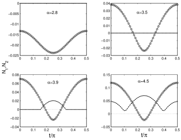
Figure 1: Time evolution of the negativity $N_{1}$ and the quantity $N_{2}$ versus $t$ with initial state being Horodecki’s state.

Now, we analyze the analytical results of negativity $N_{1}$ and quantity $N_{2}.$ One can see that when $t=\pi/2$, $N_{1}$ and $N_{2}$ are both back to the value when $t=0$, because the swap operator has no effect on the entanglement of a bipartite system. When $t=\pi$, the state has undergone a cycle. One can find when $\alpha=5/2$, all the $\lambda_{i}$ keep constant with the time. This is due to the fact that the BES with $\alpha=5/2$ is invariant under swapping operation.

From Eqs. (21) and (22), it is not difficult to find that, for arbitrary time, $N_{1}=0$ when $2\leq\alpha\leq\frac{5}{2}+\frac{2}{\sqrt{3}}\approx 3.655.$ Then, we know that in this range if $N_{2}>0$, the state is bound entangled. In Fig. 1, we plot the negativity $N_{1}$ and the quantity $N_{2}$ versus $t$ for different $\alpha$. When the initial state is a separable state ($\alpha=2.8$), one cannot generate entanglement. For $\alpha=3.5$, the initial state is bound entangled, and as time increases, the strength of bound entanglement decreases until it vanishes. After some time, the state becomes bound entangled again. Here, there is no free entanglement.

When we increase $\alpha$ to $\alpha=3.9>3.655$, the state can be made free entangled over a certain range of time within one period. After time evolution begins, The entanglement keep bounded until it becomes free. From the figure, we also see that when the initial state is free entangled ($\alpha=4.5$), the entanglement keeps free all the time. We see that the bound entanglement can be free by the time evolution.

Now, let us see the evolution of concurrence. We cannot get concurrence, but can know a lower bound. In Ref. kchen , Chen et al. derived a theorem that for any $n\otimes n$ mixed quantum state $\rho$, the concurrence $C(\rho)$satisfies

$$C(\rho)\geq\sqrt{\frac{2}{n(n-1)}}[\max(\parallel\rho^{T_{2}}\parallel,\parallel R(\rho)\parallel)-1],$$ (28)

The theorem gives the lower bound of concurrence of an arbitrary mixed state. In the case of $n=3$. From Fig. 1, we can read the time behaviors of the lower bound. For $\alpha=3.9,4.5$, the bound is always larger than zero, and it displays some singularities due to the competition between the two trace norms.

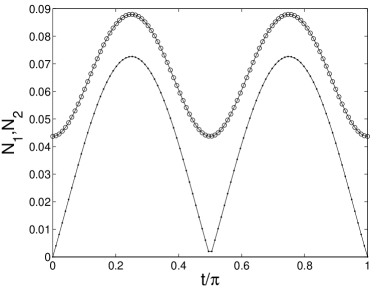
Figure 2: Time evolution of the negativity $N_{1}$ and the quantity $N_{2}$ versus $t$ with initial state being first BES constructed from UPB.

Next, we consider BES constructed from the unextendable product basis (UPB). The first BES from UPB is given by bennet ,

$$|\phi_{0}\rangle = \frac{1}{\sqrt{2}}|0\rangle(|0\rangle-|1\rangle),\ \ |\phi_{1}\rangle=\frac{1}{\sqrt{2}}(|0\rangle-|1\rangle)|2\rangle,$$

$$|\phi_{2}\rangle = \frac{1}{\sqrt{2}}|2\rangle(|1\rangle-|2\rangle),\ \ |\phi_{3}\rangle=\frac{1}{\sqrt{2}}(|1\rangle)-|2\rangle)|0\rangle,$$

$$|\phi_{4}\rangle = \frac{1}{3}(|0\rangle+|1\rangle+|2\rangle)(|0\rangle+|1\rangle+|2\rangle),$$ (29)

from which the density matrix could be expressed as

$$\rho_{{}_{UPB}}=\frac{1}{4}(I_{9\times 9}-\sum_{j=0}^{4}|\phi_{j}\rangle\langle\phi_{j}|),$$ (30)

here $I_{9\times 9}$ is the $9\times 9$ identity matrix. The second BES from UPB is given by Eq. (30) with bennet

$$|\phi_{j}\rangle = |\vec{v}_{j}\rangle\otimes|\vec{v}_{2j\text{mod}5}\rangle,j=0,...4,$$

$$|\vec{v}_{j}\rangle = \frac{2}{\sqrt{5+\sqrt{5}}}\left[\cos(2\pi j/5),\sin(2\pi j/5),\sqrt{1+\sqrt{5}}/2\right].$$

The negativity of both these two states are zero, but the trace norm is given by 1.087 and 1.098, respectively, indicating that these two states are bound entangled.

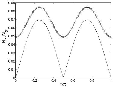
Figure 3: Time evolution of the negativity $N_{1}$ and the quantity $N_{2}$ versus $t$ with initial state being second BES constructed from UPB.

The time evolution of the two BESs are plotted in Fig. 2 and 3, respectively. There is no qualitative difference between the two plots. The bound entanglement becomes free once triggering the time evolution, namely, the bound entanglement is very fragile comparing with that in the Horodecki’s state. Also, we see that the lower bound of concurrence is determined by quantity $N_{2}$ for all time. We can free bound entanglement by the time evolution.

In conclusion, we have studied the time-evolution of BESs by two different operational approaches, namely, the partial transpose and realignment approach. The entanglement properties of time-evolution of different kind of initial BESs under the bilinear-biquadratic Hamiltonian. The analytical results of trace norms are obtained for the initial state being Horodecki’s BES at any time.

For the initial Horodecki’s BES, the state keeps bound entangled in the beginning of time evolution, while for the initial BESs constructed from UPB, the BES becomes free once the time evolution begins. The time behaviors are very different for different ‘class’ of BESs. Some BESs are relatively stable against time evolution, and some are fragile. Even a small perturbation can free the bound entanglement from UPB. The time evolution provide a new way to construct BES, and also gives a method to free bound entanglement.

This work was supported by NSFC No. 10674117 and 10405019, specialized Research Fund for the Doctoral Program of Higher Education (SRFDP) under grant No.20050335087, and the project-sponsored by SRF for ROCS and SEM. This work is partially supported by the Direct Grant of CUHK (A/C 2060286).

References

• (1) M.A. Nielsen and I.L. Chuang, Quantum Computation and Quantum Information, Cambridge University Press, Cambridge, 2000.
• (2) M. Horodecki, P. Horodecki, and R. Horodecki, Phys. Rev. Lett. 80, 5239 (1998)
• (3) V. Vedral, M. Plenio, Phys. Rev. A 57, 1619 (1998).
• (4) P. Horodecki, M. Horodecki, and R. Horodecki, Acta Phys. Slovaca 48, 141 (1998).
• (5) D. Rohrlich and S. Popescu, Phys. Rev. A 56, 3319 (1997).
• (6) M. Horodecki, P.Horodecki, and R. Horodecki, in Quantum information: An Introduction to Basic Theoretical Concepts and Experiments, edited by G. Alber et al., Springer Tracts in Modern Physics Vol. 173(Springer Verlag, Berlin, 2001), pp. 151-195.
• (7) P. Horodecki, M. Horodecki and P. Horodecki, Phys. Rev. A 63, 022310 (2001).
• (8) A. Peres, Phys. Rev. Lett. 77, 1413 (1996).
• (9) M. Horodecki, P. Horodecki, and R. Horodecki, Phys. Lett. A 223, 1 (1996).
• (10) G. Vidal and R.F. Werner, Phys. Rev. A 65 032314 (2002).
• (11) O. Rudolph, Quantum Information Processing, 4, 3 (2005).
• (12) K. Chen and L.A. Wu, Quantum. Inf. Comput. 3, 93 (2003).
• (13) It was shown by Simon (R. Simon, quant-ph/0608250) that the negative partially transposed entangled state can be also bound.
• (14) I. Affleck, T. Kennedy, E.H. Lieb and H. Tasaki, Phys, Rev. Lett.59, 799 (1987).
• (15) For instance, G. M. Zhang and X. Wang, J.Phys. A 39 (2006) 8515.
• (16) H. Fan, quant-ph/0210168.
• (17) K. Chen, S. Albeverio, and S.-M. Fei, Phys. Rev. Lett. 95, 040504 (2005).
• (18) C.H. Bennet et al, Phys. Rev. Lett. 82, 5385 (1999).