Selective entanglement breaking

Abstract

We discuss the cases where local decoherence selectively degrades one type of entanglement more than other types. A typical case is called state ordering change, in which two input states with different amounts of entanglement undergoes a local decoherence and the state with the larger entanglement results in an output state with less entanglement than the other output state. We are also interested in a special case where the state with the larger entanglement evolves to a separable state while the other output state is still entangled, which we call selective entanglement breaking. For three-level or larger systems, it is easy to find examples of the state ordering change and the selective entanglement breaking, but for two-level systems it is not trivial whether such situations exist. We present a new strategy to construct examples of two-qubit states exhibiting the selective entanglement breaking regardless of entanglement measure. We also give a more striking example of the selective entanglement breaking in which the less entangled input state has only an infinitesimal amount of entanglement.

I Introduction

Quantum entangled states on a composite system are vital resources for many quantum information protocols 1 , and it is important to understand how various entangled states are affected by decoherence when one of the local subsystems is interacted with the environment or is transferred over a noisy quantum channel. Here we focus on the cases in which the effects of such a local quantum operation/channel are different on two different kinds of entanglement. In a typical situation, one input state has a large amount of entanglement and the other one has very small entanglement, but after applying a local quantum channel on one of the systems, the entanglement in the former state is completely destroyed while the latter state is still entangled. In other words, the less entangled state is robust against the noises of the quantum channel that severely degrades the other type of entanglement.

When the dimension of Hilbert space for the local system is more than two, namely, for a three-level or larger system, such an example is easy to find 15 . Since two levels (a two-dimensional subspace) are enough to form entanglement to another system, and there are different pairs of levels to choose, it is easy to imagine a quantum channel which completely destroys the coherence between a specific pair of levels, while leaving the coherence between another pair intact. If, however, the system in question is a qubit (a two-level system), the problem becomes nontrivial because any entanglement must use the whole two-dimensional space. Hence the phenomenon of “state ordering change” by local evolution has been sought after 15 , in which the amount of entanglement $E$ satisfies

$$\displaystyle E(\hat{\omega}_{1})\geq E(\hat{\omega}_{2}),\;\;E({{\hat{\omega}}^{\prime}}_{1})\leq E({{\hat{\omega}}^{\prime}}_{2})$$ (1)

for input states $\hat{\omega}_{1},\hat{\omega}_{2}$ and the output states ${\hat{\omega}^{\prime}}_{j}=\mathcal{E}_{L}[\hat{\omega}_{j}]\ (j=1,2)$, where $\mathcal{E}_{L}=\mathcal{E}\otimes\mathcal{I}$ is a local quantum channel. Ziman and Bu$\check{\rm z}$ek have found examples of such state ordering change for a particular measure $E$ of entanglement 15 .

At this point, one must recall that the ordering between two entangled states may depend on the choice of the entanglement measure. Eisert and Plenio showed that the condition, $E^{\prime}(\hat{\omega}_{1})<E^{\prime}(\hat{\omega}_{2})\Leftrightarrow E^{\prime\prime}(\hat{\omega}_{1})<E^{\prime\prime}(\hat{\omega}_{2})$, is not always satisfied from Monte Carlo simulation ($E^{\prime},E^{\prime\prime}$ are two different entanglement measures) 11 . That is to say, there exists a pair of states with $E^{\prime}(\hat{\omega}_{1})<E^{\prime}(\hat{\omega}_{2})$ and $E^{\prime\prime}(\hat{\omega}_{1})>E^{\prime\prime}(\hat{\omega}_{2})$. Miranowicz and Grudka studied such an ambiguity in the ordering in two-qubit states for entanglement measures including negativity, concurrence, and relative entropy of entanglement 12 ; 13 . Hence a measure-dependent example is not enough to ascertain the existence of the state ordering change in a local qubit channel. For a definite answer, we need to show that Eq. (1) holds for any measure of entanglement $E$.

In this paper, we propose a general strategy to produce many examples of two-qubit states and a qubit channel showing the state ordering change for any measure of entanglement. In these examples, the output state $\hat{\omega}^{\prime}_{1}=\mathcal{E}_{L}[\hat{\omega}_{1}]$ is separable, namely, the qubit channel destroys the entanglement in state $\hat{\omega}_{1}$ completely but leaves behind part of the entanglement in state $\hat{\omega}_{2}$, which we call “selective entanglement breaking”. We further show that a particular example constructed from the above strategy exhibits a more striking feature that the channel breaks entanglement in $\hat{\omega}_{1}$ selectively even when the input state $\hat{\omega}_{2}$ has an infinitesimal amount of entanglement.

The construction of the paper is as follows. In Sec. II, we give a trivial example of two-qutrit states and a qutrit channel showing the selective entanglement breaking. We also give precise definitions of the three relevant phenomena: state ordering change, selective entanglement breaking, and strong selective entanglement breaking. In the main part of the paper, Sec. III, we present a strategy for finding examples of two-qubit states and a qubit channel showing the selective entanglement breaking. We also construct a specific example and show that it exhibits the strong selective entanglement breaking. In Sec. IV, we show there is no selective entanglement breaking for two-qubit pure states. In Sec. V, we consider a family of entanglement measures for which the state ordering change can be discussed with a strict inequality. Finally Sec. VI concludes the paper.

II Two-qutrit state ordering change

Let us consider the case where the local system is a qutrit, namely, the dimension of the Hilbert space is three. We can easily find an example of two-qutrit states and a qutrit channel showing the state ordering change. Consider two pure states $|{\psi_{1}}\rangle=\sqrt{1/2}(|{11}\rangle+|{22}\rangle)$ and $|{\psi_{2}}\rangle=\sqrt{q}|{00}\rangle+\sqrt{1-q}|{11}\rangle$ ($0<q<1$). Suppose that the local channel $\mathcal{E}$ applied to the first system is represented by Kraus operators (the operator-sum representation): $\mathcal{E}(\hat{\rho})=\sum_{j}\hat{M}_{j}\hat{\rho}\hat{M}_{j}^{\dagger}$, where $\hat{M}_{0}=|{0}\rangle\langle{0}|+|{1}\rangle\langle{1}|$ and $\hat{M}_{1}=|{2}\rangle\langle{2}|$. After applying $\mathcal{E}_{L}=\mathcal{E}\otimes\mathcal{I}$ to the two input states, we obtain a separable state $\hat{\rho}^{\rm{out}}_{1}=(|{11}\rangle\langle{11}|+|{22}\rangle\langle{22}|)/2$ for the first input state, but the second input state remains unaltered, $\hat{\rho}^{\rm{out}}_{2}=|{\psi_{2}}\rangle\langle{\psi_{2}}|$.

In this example, the input state $|{\psi_{1}}\rangle$ can be transformed to $|{\psi_{2}}\rangle$ by local operations and classical communication (LOCC). One of the parties applies a local filter described by Kraus operators $\hat{A}_{0}=|{0}\rangle\langle{0}|+\sqrt{1-q}|{1}\rangle\langle{1}|+\sqrt{q}|{2}\rangle\langle{2}|$ and $\hat{A}_{1}=\sqrt{q}|{1}\rangle\langle{1}|+\sqrt{1-q}|{2}\rangle\langle{2}|$, and classically communicate the outcome (0 or 1) to the other party. Then, local unitary operations can transform the filtered states as $\sqrt{1-q}|{11}\rangle+\sqrt{q}|{22}\rangle{\longrightarrow}\sqrt{q}|{00}\rangle+\sqrt{1-q}|{11}\rangle$ and $\sqrt{q}|{11}\rangle+\sqrt{1-q}|{22}\rangle{\longrightarrow}\sqrt{q}|{00}\rangle+\sqrt{1-q}|{11}\rangle$. We can also transform $\hat{\rho}^{\rm{out}}_{2}$ to $\hat{\rho}^{\rm{out}}_{1}$ by LOCC, since the latter is separable. These observations assure that we have $E(\psi_{1})\geq E(\psi_{2})$ and $E(\hat{\rho}^{\rm{out}}_{1})\leq E(\hat{\rho}^{\rm{out}}_{2})$ for any entanglement measure $E$ as long as it satisfies

(i)Monotonicity under LOCC, LOCC cannot increase the entanglement, namely, if the state $\hat{\rho}^{AB}$ is transformed into $\hat{\sigma}^{AB}$ by LOCC, $E(\hat{\rho}^{AB})\geq E(\hat{\sigma}^{AB})$.

We see that this trivial example shows the state ordering change regardless of the choice of entanglement measure, which we define formally as

State ordering change — A local quantum channel $\mathcal{E}_{L}=\mathcal{E}\otimes\mathcal{I}$ and two input states $\hat{\omega}_{1}$ and $\hat{\omega}_{2}$ satisfy

$$E(\hat{\omega}_{1})\geq E(\hat{\omega}_{2}),\;\;E(\mathcal{E}_{L}[\hat{\omega}_{1}])\leq E(\mathcal{E}_{L}[\hat{\omega}_{2}])$$ (2)

for any entanglement measure $E$ satisfying the monotonicity under LOCC, and among such measures, there exists a measure $E^{\prime}$ satisfying

$$E^{\prime}(\hat{\omega}_{1})>E^{\prime}(\hat{\omega}_{2}),\;\;E^{\prime}(\mathcal{E}_{L}[\hat{\omega}_{1}])<E^{\prime}(\mathcal{E}_{L}[\hat{\omega}_{2}]).$$ (3)

Here we cannot demand the strict inequality to hold for any measure, since the property (i) cannot exclude a trivial measure which is constant for any state whether it is entangled or not. If we are to require the strict inequality, we need to restrict the allowed entanglement measures, which will be discussed in Sec. V.

In the above example of two-qutrit state ordering change, the entanglement in the state $\omega_{1}$ is completely destroyed by the channel. In this paper, we define such cases as follows:

Selective entanglement breaking — The state ordering change occurs with one of the output states being separable.

Moreover, in the trivial example considered here, the entanglement in state $|\psi_{2}\rangle$ is preserved no matter how small its entanglement is. This implies that the quantum channel selectively destroys the type of entanglement held in a state $\hat{\omega}_{1}$, while it does not completely destroy entanglement held in another state $\hat{\omega}_{2}$ even when its entanglement of formation 20 , $E_{f}(\hat{\omega}_{2})$, is infinitesimal. Here we will define such a phenomenon in the following way.

Strong selective entanglement breaking — A local quantum channel $\mathcal{E}_{L}=\mathcal{E}\otimes\mathcal{I}$, an input state $\hat{\omega}_{1}$, and a sequence of input states $\{\hat{\omega}_{j}\}_{j=2,3\ldots\infty}$ satisfy (a) $E(\hat{\omega}_{1})\geq E(\hat{\omega}_{2})\geq E(\hat{\omega}_{3})\geq\cdots$ for any measure $E$ satisfying (i), (b) There is a measure $E^{\prime}$ such that $E^{\prime}(\hat{\omega}_{1})>E^{\prime}(\hat{\omega}_{2})$ and $E^{\prime}(\mathcal{E}_{L}[\hat{\omega}_{1}])<E^{\prime}(\mathcal{E}_{L}[\hat{\omega}_{j}])$ for any $j\geq 2$, (c) $\lim_{j\to\infty}{E_{f}}(\hat{\omega}_{j})=0$, and (d) $\mathcal{E}_{L}[\hat{\omega}_{1}]$ is separable.

In the three-level system considered here or in larger systems, the existence of the state ordering change is trivial, and even the existence of the strong selective entanglement breaking is also trivial as shown above. The next section will deal with the nontrivial question for the case of a two-level system.

III Two-qubit state ordering change

In this section, we show an example of the selective entanglement breaking where the local system is a qubit. For two-qutrit system, it was not difficult to find the example of the strong selective entanglement breaking. This is because for three-level or larger systems we can preserve entanglement even if we apply a projector onto a two-dimensional subspace. But for a two-level input system, we cannot preserve entanglement by nontrivial projections. It is thus difficult to find an example of two-qubit selective entanglement breaking along the line used in the previous section.

Our strategy to find such an example is as follows. First we consider an entangled mixed state $\hat{\rho}^{AB}$ and a qubit channel $\mathcal{E}_{\lambda}$ with a parameter $\lambda$ representing the amount of the noise introduced by the channel. After applying the local channel to the input state $\hat{\rho}^{AB}$, we calculate the negativity 4 ; 5 of state $\mathcal{E}_{\lambda}\otimes\mathcal{I}(\hat{\rho}^{AB})$ as a function of $\lambda$ to find the value of $\lambda=\lambda_{\rm sep}$ at which the state becomes separable. Next, going back to the original state $\hat{\rho}^{AB}$, we apply a local unitary $\hat{U}$ to the first system to produce $\hat{\rho}^{AB}_{U}\equiv(\hat{U}\otimes\hat{I})\hat{\rho}^{AB}(\hat{U}^{\dagger}\otimes\hat{I}^{\dagger})$. We again calculate the critical value $\lambda_{\rm sep}$ for this state. The success of our strategy rests on whether the critical value $\lambda_{\rm sep}$ changes depending on the choice of the unitary $\hat{U}$. Once we find such a dependency, we can construct an example of the selective entanglement breaking as follows. Without loss of generality, we can assume that there is a value of $\lambda$ for which $\mathcal{E}_{\lambda}\otimes\mathcal{I}(\hat{\rho}^{AB}_{U})$ is separable, while the negativity of state $\mathcal{E}_{\lambda}\otimes\mathcal{I}(\hat{\rho}^{AB})$ is strictly positive. Then, we consider an LOCC operation $\mathcal{E}^{\prime}_{\epsilon}$ with parameter $\epsilon$ representing the strength of the noise ($\mathcal{E}^{\prime}_{0}=\mathcal{I}\otimes\mathcal{I}$), and apply it to state $\hat{\rho}^{AB}$ to obtain $\hat{\rho}^{AB}_{\epsilon}\equiv\mathcal{E}^{\prime}_{\epsilon}(\hat{\rho}^{AB})$. If $\epsilon$ is small enough but nonzero, we have $N(\hat{\rho}^{AB}_{\epsilon})<N(\hat{\rho}^{AB})=N(\hat{\rho}^{AB}_{U})$ while the negativity of the new state $\mathcal{E}_{\lambda}\otimes\mathcal{I}(\hat{\rho}^{AB}_{\epsilon})$ should still be strictly positive, namely, $N(\mathcal{E}_{\lambda}\otimes\mathcal{I}(\hat{\rho}^{AB}_{\epsilon}))>0=N(\mathcal{E}_{\lambda}\otimes\mathcal{I}(\hat{\rho}^{AB}_{U}))$. Hence, for the negativity, the strict inequality (3) is satisfied (see Fig.1). On the other hand, we can convert $\hat{\rho}^{AB}_{U}$ to $\hat{\rho}^{AB}_{\epsilon}$ by LOCC ($\hat{U}^{-1}\otimes\hat{I}$ followed by $\mathcal{E}^{\prime}_{\epsilon}$), and we can also convert $\mathcal{E}_{\lambda}\otimes\mathcal{I}(\hat{\rho}^{AB}_{\epsilon})$ to $\mathcal{E}_{\lambda}\otimes\mathcal{I}(\hat{\rho}^{AB}_{U})$ by LOCC since the latter is separable. Hence, from the monotonicity (i), the inequality (2) holds for any measure $E$.

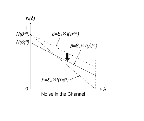
Figure 1: Strategy to find examples of the selective entanglement breaking. We use negativity $N(\hat{\rho})$ as an entanglement measure, since it is easy to calculate. Slight decrease in the degree of entanglement (the arrow) is done by LOCC, and hence the order of the two input states is measure-independent. The order of the two output states is also measure-independent, since one of them is separable.

Let us show a specific example using the above strategy. First we consider a mixed entangled state,

$$\displaystyle\hat{\rho}_{1}^{\rm in}=\frac{2}{3}|{\Phi_{+}}\rangle\langle{\Phi_{+}}|+\frac{1}{3}|{00}\rangle\langle{00}|,$$ (4)

where $|{\Phi_{+}}\rangle=\sqrt{1/2}(|{00}\rangle+|{11}\rangle)$. Consider a local unitary on the first system $A$,

$$\displaystyle\hat{U}_{A}=\frac{1}{\sqrt{2}}\left(\begin{array}[]{cc}1&-1\\ 1&1\\ \end{array}\right),$$ (7)

which is the rotation around $Y$ axis by $\theta=\pi/2$ on the Bloch sphere. Let $\hat{\rho}_{2}^{\rm{in}}=(\hat{U}_{A}\otimes\hat{I}_{B})\hat{\rho}^{\rm{in}}_{1}(\hat{U}_{A}^{\dagger}\otimes\hat{I}_{B}^{\dagger})$, which is written on the basis $\{|00\rangle,|01\rangle,|10\rangle,|11\rangle\}$ in the matrix form

$$\displaystyle\hat{\rho}_{2}^{\rm{in}}=\frac{1}{6}\left(\begin{array}[]{cccc}2&-1&2&1\\ -1&1&-1&-1\\ 2&-1&2&1\\ 1&-1&1&1\\ \end{array}\right).$$ (12)

As the local quantum channel applied to system $A$, we take a phase damping channel represented by two Kraus operators

$$\displaystyle\hat{E}_{0}=\left(\begin{array}[]{cccc}1&0\\ 0&\sqrt{1-\lambda}\\ \end{array}\right),\ \ \hat{E}_{1}=\left(\begin{array}[]{cccc}0&0\\ 0&\sqrt{\lambda}\\ \end{array}\right),$$ (17)

where $0\leq\lambda\leq 1$. For an input two-qubit state $\hat{\rho}^{\rm{in}}$, the output of the phase damping channel is given by $\hat{\rho}^{\rm{out}}=(\hat{E}_{0}\otimes\hat{I})\hat{\rho}^{\rm{in}}(\hat{E}_{0}^{\dagger}\otimes\hat{I}^{\dagger})+(\hat{E}_{1}\otimes\hat{I})\hat{\rho}^{\rm{in}}(\hat{E}_{1}^{\dagger}\otimes\hat{I}^{\dagger})$. For the two input states $\hat{\rho}^{\rm{in}}_{1}$ and $\hat{\rho}^{\rm{in}}_{2}$, the output states are calculated as

$$\displaystyle\hat{\rho}_{1}^{\rm{out}} = \frac{1}{3}\left(\begin{array}[]{cccc}2&0&0&\sqrt{1-\lambda}\\ 0&0&0&0\\ 0&0&0&0\\ \sqrt{1-\lambda}&0&0&1\\ \end{array}\right),$$ (22)

$$\hat{\rho}_{2}^{\rm{out}} = \frac{1}{6}\left(\begin{array}[]{cccc}2&-1&2\sqrt{1-\lambda}&\sqrt{1-\lambda}\\ -1&1&-\sqrt{1-\lambda}&-\sqrt{1-\lambda}\\ 2\sqrt{1-\lambda}&-\sqrt{1-\lambda}&2&1\\ \sqrt{1-\lambda}&-\sqrt{1-\lambda}&1&1\\ \end{array}\right).$$ (27)

The negativity for a bipartite state $\hat{\rho}$ is defined by

$$\displaystyle N(\hat{\rho})=\max{\left\{0,-2\mu_{\rm{min}}\right\}},$$ (29)

where $\mu_{\rm{min}}$ is the minimum of the eigenvalues of the partial transpose of state $\hat{\rho}$ 4 ; 5 . For two-qubit states, it has the range from 0 (separable) to 1 (maximally entangled). The negativity of the two output states $\hat{\rho}_{1}^{\rm{out}}$ and $\hat{\rho}_{2}^{\rm{out}}$ are

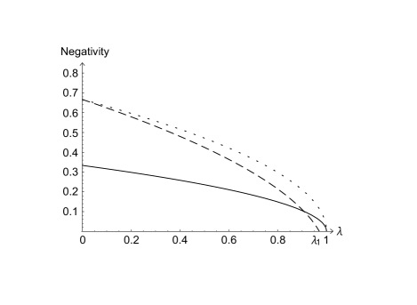
Figure 2: Example of the selective entanglement breaking. The negativities of $\hat{\rho}_{1}^{\rm{out}}$, $\hat{\rho}_{2}^{\rm{out}}$, $\hat{\rho}_{3}^{\rm{out}}$ ($t=1/3$) are indicated by the dotted curve, the dashed curve, and the solid curve, respectively.

$$\displaystyle N(\hat{\rho}_{1}^{\rm{out}}) = \frac{2}{3}\sqrt{1-\lambda},$$ (30)

$$N(\hat{\rho}_{2}^{\rm{out}}) = \frac{1}{6}\Bigl{(}-3+3\sqrt{1-\lambda}+\sqrt{10+6\sqrt{1-\lambda}-5\lambda}\Bigr{)},$$

which are shown in Fig. 2.

When the noise parameter of the quantum channel is $\lambda=\lambda_{1}\equiv-16+12\sqrt{2}\approx 0.97$, $N(\hat{\rho}_{2}^{\rm{out}})=0$, and $N(\hat{\rho}_{1}^{\rm{out}})_{|\lambda=\lambda_{1}}=2(3-2\sqrt{2})/3\approx 0.11>0$. Then we decrease $N(\hat{\rho}_{1}^{\rm{in}})$ using LOCC. Specifically, we consider an operation in which the state is replaced by $|{00}\rangle$ with probability $\epsilon$. Applying this operation to $\hat{\rho}_{1}^{\rm{in}}$, we have

$$\displaystyle\hat{\rho}_{3}^{\rm{in}}=t|{\Phi_{+}}\rangle\langle{\Phi_{+}}|+(1-t)|{00}\rangle\langle{00}|,$$ (32)

where $t=2(1-\epsilon)/3<2/3$. Calculating in a similar way, we obtain the negativity of the output state as

$$N(\hat{\rho}_{3}^{\rm{out}})=t\sqrt{1-\lambda}.$$ (33)

The case with $t=1/3$ is shown in Fig. 2.

As explained for the general strategy, $E(\hat{\rho}_{3}^{\rm{in}})\leq E(\hat{\rho}_{2}^{\rm{in}})$ and $E(\hat{\rho}_{3}^{\rm{out}})\geq E(\hat{\rho}_{2}^{\rm{out}})$ hold for any entanglement measure satisfying the monotonicity (i). On the other hand, $N(\hat{\rho}_{3}^{\rm{in}})<N(\hat{\rho}_{2}^{\rm{in}})$ holds for $t<2/3$ and $N(\hat{\rho}_{3}^{\rm{out}})>N(\hat{\rho}_{2}^{\rm{out}})$ holds for $t>0$. Hence the phase damping channel with $\lambda=\lambda_{1}$ and the states $\hat{\rho}_{2}^{\rm{in}}$ and $\hat{\rho}_{3}^{\rm{in}}$ with $0<t<2/3$ exhibit the selective entanglement breaking.

In the limit of $t\rightarrow 0$, the state $\hat{\rho}_{3}^{\rm{in}}$ becomes separable. But as long as $t>0$, the output state is still entangled, and the state ordering change occurs. Hence the particular example here exhibits not only the selective entanglement breaking, but also the strong selective entanglement breaking.

IV No selective entanglement breaking exists for two-qubit pure states

In the previous section, we present a specific example of selective entanglement breaking in which the two input states are mixed states. In fact, we cannot find pure-state examples by our strategy. The reason is closely related to the following general property of qubit channels: if a two-qubit pure entangled state becomes separable after one of the qubit passes through a qubit channel, then the channel is an entanglement breaking channel 16 ; 17 , namely, the channel destroys the entanglement of any input state. We can prove it as follows.

Consider a two-qubit pure state $|{\psi_{\rm{in}}}\rangle=\alpha|{00}\rangle+\beta|{11}\rangle$, where ${\alpha}^{2}+{\beta}^{2}=1$, and suppose that $|{\psi_{\rm{in}}}\rangle$ becomes separable state $\hat{\rho}_{\rm sep}$ after the application of a qubit channel. Imagine we further apply a local filter, which is described by the Kraus operator $\hat{M}_{0}=\beta|{0}\rangle\langle{0}|+\alpha|{1}\rangle\langle{1}|$, to the second qubit. The state after the successful filtering, $\hat{\sigma}_{\rm sep}\equiv(\hat{I}\otimes\hat{M}_{0})\hat{\rho}_{\rm sep}(\hat{I}\otimes\hat{M}_{0})^{\dagger}$, is separable since $\hat{\rho}_{\rm sep}$ is separable. Now notice that even if we apply the local filter first and then apply the one-qubit channel, the final state should be the same because they are operations on different systems. In this case, the state after the successful filtering is a maximally entangled state $\sqrt{1/2}(|{00}\rangle+|{11}\rangle)$, which evolves into the separable state $\hat{\sigma}_{\rm sep}$ after the application of the qubit channel. Hence the channel must be an entanglement breaking channel.

This property of qubit channels immediately tells us that there is no selective entanglement breaking with the input two-qubit state $\hat{\omega}_{1}$, which is to be broken, being a pure state. Our strategy in Sec. III does not work for pure $\hat{\rho}^{AB}$ because $\lambda_{\rm sep}$ is the same for any unitary operation $\hat{U}$. Although there is no selective entanglement breaking for pure two-qubit states, the present argument does not exclude the possibility of the state ordering change for two pure two-qubit input states.

For a system with dimension $d$ larger than two, a straightforward extension of the above proof shows that a local channel is entanglement breaking if a pure entangled state with full local rank (the marginal density operator having rank $d$) is broken by the channel. This leaves the possibility of having the selective entanglement breaking of pure states with a small local rank, as in the trivial example shown in Sec. II.

V State ordering change with strict inequality

As discussed in Sec. II, not all of the entanglement measures satisfying the monotonicity (i) fulfill the strict inequality (3). Here we show that, in the example in Sec. III, the strict inequality (3) holds for a wide range of measures specified by a set of additional conditions which are often considered to be desirable as a measure of entanglement. We consider the measures satisfying the following properties:

(i^′)Monotonicity under LOCC on average, if LOCC transforms $\hat{\rho}^{AB}$ into a state $\hat{\rho}^{AB}_{i}$ with probability $p_{i}$, the entanglement does not increase on average, i.e. $E(\hat{\rho}^{AB})\geq\sum_{i}p_{i}E(\hat{\rho}^{AB}_{i})$;
(ii)Vanishing on separable states, $E(\hat{\rho}^{AB})=0$ if $\hat{\rho}^{AB}$ is separable;
(iii)Normalization, $E(|\Phi\rangle\langle\Phi|)=1$, where $|\Phi\rangle=\sqrt{1/2}(|{00}\rangle+|{11}\rangle)$;
(iv)Convexity, $E(\sum_{i}p_{i}\hat{\rho}^{AB}_{i})\leq\sum_{i}p_{i}E(\hat{\rho}^{AB}_{i})$;
(v)Partial additivity, $E(\hat{\rho}^{\otimes n})=nE(\hat{\rho})$;
(vi)Partial continuity, if state $\hat{\rho}_{n}$ approaches ${\hat{\psi}}^{\otimes n}$ for large $n$: $\langle{{\psi}^{\otimes n}}|\hat{\rho}_{n}|{{\psi}^{\otimes n}}\rangle\to 1$ for $n\to\infty$, then $|E({\hat{\psi}}^{\otimes n})-E(\hat{\rho}_{n})|/n\to 0$.

It is shown that for any measure $E$ satisfying the above set of conditions, the following inequality holds for any state $\hat{\rho}$ 18 :

$${E_{D}}(\hat{\rho})\leq E(\hat{\rho})\leq{E_{C}}(\hat{\rho}),$$ (34)

where ${E_{D}}(\hat{\rho})$ is the distillable entanglement 21 and ${E_{C}}(\hat{\rho})$ is the entanglement cost 19 . Using this relation, we can easily see that $E(\hat{\rho}_{3}^{\rm{out}})>E(\hat{\rho}_{2}^{\rm{out}})=0$ since $\hat{\rho}_{3}^{\rm{out}}$ is entangled and any two-qubit entangled state is distillable 14 , namely, $0<{E_{D}}(\hat{\rho}_{3}^{\rm{out}})\leq E(\hat{\rho}_{3}^{\rm{out}})$. We can also prove $E(\hat{\rho}_{3}^{\rm{in}})<E(\hat{\rho}_{2}^{\rm{in}})$ for $0<t<0.495\cdots$ as follows. From Eq. (34), we have

$$E(\hat{\rho}_{3}^{\rm{in}})\leq{E_{C}}(\hat{\rho}_{3}^{\rm{in}}),\ \ {E_{D}}(\hat{\rho}_{2}^{\rm{in}})\leq E(\hat{\rho}_{2}^{\rm{in}}),$$ (35)

and hence what we need is an upper bound on ${E_{C}}(\hat{\rho}_{3}^{\rm{in}})$ and a lower bound on ${E_{D}}(\hat{\rho}_{2}^{\rm{in}})$.

The entanglement cost ${E_{C}}(\hat{\rho})$ is upper-bounded 19 by the entanglement of formation ${E_{f}}(\hat{\rho})$ 20 , which can be computed through the concurrence $C(\hat{\rho})$ 3 as

$${E_{f}}(\hat{\rho})=H[\frac{1}{2}(1+\sqrt{1-{C^{2}}(\hat{\rho})})],$$ (36)

$$H(p)=-p\log p-(1-p)\log(1-p).$$ (37)

Using this relation, we have

$${E_{C}}(\hat{\rho}_{3}^{\rm{in}}) \leq {E_{f}}(\hat{\rho}_{3}^{\rm{in}})$$ (38)

$$= H[\frac{1}{2}(1+\sqrt{1-t^{2}})].$$ (39)

A lower bound of $E_{D}$ is given 20 ; 21 as

$$g(\hat{\rho})=1+\sum_{x}\lambda_{x}\log\lambda_{x}\leq{E_{D}}(\hat{\rho}),$$ (40)

where $\lambda_{x}$ are the diagonal entries of the matrix form of $\hat{\rho}$ on a Bell basis. Since $\hat{\rho}_{2}^{\rm{in}}$ is rewritten on a Bell basis as

$$\displaystyle\frac{1}{6}\left(\begin{array}[]{cccc}5&0&0&1\\ 0&0&0&0\\ 0&0&0&0\\ 1&0&0&1\\ \end{array}\right),$$ (45)

$g(\hat{\rho}_{2}^{\rm{in}})=1-H(1/6)$ $(\approx 0.35)$. Solving $1-H(1/6)>H[(1+\sqrt{1-t^{2}})/2]$ numerically, we find that

$${E_{f}}(\hat{\rho}_{3}^{\rm{in}})<g(\hat{\rho}_{2}^{\rm{in}}),$$ (46)

holds for $0<t<0.495\cdots$. From Eqs. (35), (38), (40), and (46), we obtain

$$E(\hat{\rho}_{3}^{\rm{in}})<E(\hat{\rho}_{2}^{\rm{in}}).$$ (47)

Hence for $0<t<0.495\cdots$, the strict inequality (3) holds for the family of entanglement measures satisfying the properties (i^′), (ii)-(vi).

VI Conclusion

We have shown examples of a local qubit channel exhibiting the selective entanglement breaking and an example with the strong selective entanglement breaking. These results imply that even for the system as small as a qubit, a quantum channel/operation can have a preference over which kind of entanglement to break. In our examples, the ordering with respect to entanglement is determined by the transformability through LOCC operations, and hence is defined solely by the property of monotonicity. This makes our results independent of the choice of the entanglement measure. We have also shown that the ordering change with a strict inequality holds for a family of measures satisfying a set of plausible conditions.

- (1) M. A. Nielsen and I. L. Chuang, Quantum Computation and Quantum Information, (Cambridge University Press, Cambridge, England, 2000).
- (2) M. Ziman and V. Buek, Phys. Rev. A 73, 012312 (2006).
- (3) J. Eisert and M. B. Plenio, J. Mod. Opt. 46,145 (1999).
- (4) A. Miranowicz and A. Grudka, Phys. Rev. A 70, 032326 (2004).
- (5) A. Miranowicz and A. Grudka, J. Opt. B: Quantum Semiclass. Optics 6 (2004) 542-548.
- (6) C. H. Bennett, D. P. Di Vincenzo, J. Smolin, and W. K. Wootters, Phys. Rev. A 54, 3824 (1996).
- (7) A. Peres, Phys. Rev. Lett. 77, 1413 (1996).
- (8) M. Horodecki, P. Horodecki, and R. Horodecki, Phys. Lett. A 223, 1 (1996).
- (9) M. Horodecki, P. W. Shor, and M. B. Ruskai, quant-ph/0301031, Rev. Math. Phys. 15, 629-641 (2003).
- (10) M. B. Ruskai, quant-ph/0302032, Rev. Math. Phys. 15, 643-662 (2003).
- (11) M. Horodecki, P. Horodecki, and R. Horodecki, Phys. Rev. Lett. 84, 2014 (2000).
- (12) C. H. Bennett, G. Brassard, S. Popescu, B. Schumacher, J. Smolin, and W. K. Wootters, Phys. Rev. Lett. 76, 722 (1996).
- (13) P. M. Hayden, M. Horodecki, and B. M. Terhal, J. Phys. A 34, 6891 (2001).
- (14) M. Horodecki, P. Horodecki, and R. Horodecki, Phys. Rev. Lett. 78, 574 (1997).
- (15) W. K. Wootters, Phys. Rev. Lett. 80, 2245 (1998).