Entanglement generation in atoms immersed in a thermal bath of external quantum scalar fields with a boundary

Abstract

We examine the entanglement creation between two mutually independent two-level atoms immersed in a thermal bath of quantum scalar fields in the presence of a perfectly reflecting plane boundary. With the help of the master equation that describes the evolution in time of the atom subsystem obtained, in the weak-coupling limit, by tracing over environment (scalar fields) degrees of freedom, we find that the presence of the boundary may play a significant role in the entanglement creation in some circumstances and the new parameter, the distance of the atoms from the boundary, besides the bath temperature and the separation between the atoms, gives us more freedom in manipulating entanglement generation. Remarkably, the final remaining entanglement in the equilibrium state is independent of the presence of the boundary.

I Introduction

Quantum entanglement has now been recognized as a key resource in quantum information science information , since it plays a primary role in quantum communication Bennett , quantum teleportation telportation , quantum cryptography cryptography and so on. An interesting issue in the discussions for the essence of entanglement, which has attracted a lot of attention, is the relationship between entanglement and environment. It is known that an environment usually leads to decoherence and noise, which may cause entanglement that might have been created before to disappear. However, in certain circumstances, the environment may enhance entanglement rather than destroying it pr1 ; pr2 ; pr3 ; pr4 ; pr5 ; pr6 . The reason is that an external environment can also provide an indirect interaction between otherwise totally uncoupled subsystems through correlations that exist. For example, correlations in vacuum fluctuations or fluctuations at finite temperature can provide such an interaction, when entanglement generation is considered in systems in external quantum fields.

Recently Benatti et al have discussed, in the framework of open systems, entanglement generation for two, independent uniformly accelerating two-level atoms interacting with a set of scalar fields in vacuum. In the weak coupling limit, the completely positive dynamics for the atoms as a subsystem has been derived by tracing over the field degrees of freedom Benatti1 , and there it has been shown that the asymptotic equilibrium state of the atoms turns out to be entangled even if the initial state is separable. Similar results have been obtained by considering two atoms immersed in a thermal bath of scalar particles at a finite temperature Benatti2 , where, in contrast to Ref. Benatti1 , two atoms are assumed to be at a finite separation. It is found that for any fixed, finite separation, there always exists a temperature below which entanglement generation occurs as soon as time starts to become nonzero and for the vanishing separation the entanglement thus generated persists even in the late-time asymptotic equilibrium state. Therefore, one can manipulate the entanglement production by controlling two controllable parameters: the bath temperature and the separation of the atoms.

In the above studies, the field correlation functions that characterize the fluctuations of fields play a very important role in determining whether entanglement is generated. On the other hand, it is well-known that the presence of boundaries in a flat spacetime modifies the fluctuations of quantum fields, and it has been demonstrated that this modification can lead to a lot of novel effects, such as the Casimir effect cas , the light-cone fluctuations when gravity is quantized YU , the Brownian (random) motion of test particles in an electromagnetic vacuum yu2 , and the modification for the radiative properties of uniformly accelerated atoms yu3 .

A question then arises naturally as to what happens to the entanglement generation if the field correlations are modified by the presence of a reflecting boundary. Now we have one more controllable parameter other than the separation and the bath temperature, i.e., the distance of the atoms from the boundary and another interesting question is what is the role that the new parameter plays in the entanglement generation. These are questions we are going to address in the present paper. We shall examine the entanglement generation of two non-interacting two-level atoms immersed in a thermal bath of scalar particles subjected to a perfectly reflecting plane boundary. With the help of the master equation that describes the evolution of the open system (atoms plus external thermal fields) in time, we find that the presence of the boundary may play an significant role in controlling the entanglement creation in some circumstances and the new parameter, the distance of the atoms from the boundary, gives one more freedom in controlling the entanglement generation. It is, however, interesting that the probable remaining entanglement for the asymptotic equilibrium state at late times is not dependent on the presence of the boundary.

II Two Atom Master Equation

The system we shall examined is composed of two independent two-level atoms in weak interaction with a set of massless quantum scalar fields at a finite temperature $T$. We assume that a perfectly reflecting plane boundary for the scalar fields is located at $z=0$ in space and one atom is placed at point ${\bf x}_{1}$ and the other at ${\bf x}_{2}$. Without loss of generality, we take the total Hamiltonian to have the form

$$H=H_{s}+H_{\phi}+\lambda\;H^{\prime}\;.$$ (1)

Here $H_{s}$ is the Hamiltonian of the two atoms,

$$H_{s}=H_{S}^{(1)}+H_{s}^{(2)},\ \ H_{s}^{(\alpha)}={\omega\over 2}\,n_{i}\,\sigma_{i}^{(\alpha)},\quad(\alpha=1,2),\ \$$ (2)

where $\sigma_{i}^{(1)}=\sigma_{i}\otimes{\sigma_{0}},\ \ \sigma_{i}^{(2)}={\sigma_{0}}\otimes\sigma_{i}$, $\sigma_{i},(i=1,2,3)$ are the Pauli matrices, $\sigma_{0}$ the $2\times 2$ unit matrix, $\mathbf{n}=(n_{1},n_{2},n_{3})$ a unit vector, $\omega$ the energy level spacing, and summation over repeated index is implied. $H_{\phi}$ is the standard Hamiltonian of massless, free scalar fields, details of which is not relevant here and $H^{\prime}$ is the Hamiltonian that describes the interaction between the two atoms with the external scalar fields which is assumed to be weak. The general form for $H^{\prime}$ can be written as

$$H^{\prime}=\sum_{\mu=0}^{3}\,[(\sigma_{\mu}\otimes\sigma_{0})\Phi_{\mu}(t,{\bf x}_{1})+(\sigma_{0}\otimes\sigma_{\mu})\Phi_{\mu}(t,{\bf x}_{2})\,]\;.$$ (3)

Now we assume that the scalar fields can be expanded as

$$\Phi_{\mu}(x)=\sum^{N}_{a=1}\,[\chi_{\mu}^{a}\phi^{(-)}(x)+(\chi_{\mu}^{a})^{*}\phi^{(+)}(x)]\;,$$ (4)

where $\phi^{(\pm)}(x)$ are positive and negative energy field operators of the massless scalar field, and $\chi_{\mu}^{a}$ are complex coefficients that ”embed” the field modes into the two-dimensional detector Hilbert space and play the role of generalized coupling constants Benatti1 . It should be pointed out that the coupling constant $\lambda$ in (1) is small, and this is consistent with the assumption that the interaction of the atom with the scalar fields is weak.

It is well-known that the evolution of the total system density (i.e., the two atoms plus the environment) in time obeys the Liouville equation $\partial_{t}\rho_{tot}(t)=-i[H,\rho_{tot}(t)]$ with the initial total density having a generic form $\rho_{tot}(0)=\rho(0)\otimes\rho_{B}$, where the environment fields are taken to be in a thermal state characterized by $\rho_{B}$ and the atom in an initial state $\rho(0)$. Since our interest is in the dynamics for the two atoms only, we must trace over the environment degrees of freedom and concentrate on the analysis of the reduced time evolution, $\rho(t)=Tr_{\phi}[\rho_{tot}]$. Provided that the field correlations decay sufficiently fast at large time separations, or much faster than the characteristic evolution time of the subsystem alone, the reduced density of the two-atom subsystem can be proven, in the limit of weak-coupling, to obey an equation in the Kossakowski-Lindblad form Lindblad ; Benatti1 ; Benatti2 ; pr5

$${\partial\rho(t)\over\partial t}=-i\big{[}H_{\rm eff},\,\rho(t)\big{]}+{\cal L}[\rho(t)]\ ,$$ (5)

with

$$H_{\rm eff}=H_{S}-\frac{i}{2}\sum_{\alpha,\beta=1}^{2}H_{ij}^{(\alpha\beta)}\ \sigma_{i}^{(\alpha)}\,\sigma_{j}^{(\beta)}\ ,$$ (6)

and

$${\cal L}[\rho]={1\over 2}\sum_{\alpha,\beta=1}^{2}C_{ij}^{(\alpha\beta)}\big{[}2\,\sigma_{j}^{(\beta)}\rho\,\sigma_{i}^{(\alpha)}-\sigma_{i}^{(\alpha)}\sigma_{j}^{(\beta)}\,\rho-\rho\,\sigma_{i}^{(\alpha)}\sigma_{j}^{(\beta)}\big{]}\ .$$ (7)

The coefficients of the matrix $C_{ij}^{(\alpha\beta)}$ and $H_{ij}^{(\alpha\beta)}$ are determined by the field correlation functions in the thermal state $\rho_{\beta}$:

$$\mathrm{}G_{ij}^{\alpha\beta}(t-t^{\prime})={}_{\beta}\langle\Phi_{i}(t,\mathbf{x}_{\alpha})\Phi_{j}(t^{\prime},\mathbf{x}_{\beta})\rangle_{\beta}\;.$$ (8)

The corresponding Fourier and Hilbert transforms read respectively

$${\cal G}_{ij}^{(\alpha\beta)}(\lambda)=\int_{-\infty}^{\infty}dt\,e^{i{\lambda}t}\,G_{ij}^{(\alpha\beta)}(t)\;,$$ (9)

$${\cal K}_{ij}^{(\alpha\beta)}(\lambda)=\int_{-\infty}^{\infty}dt\,{\rm sign}(t)\,e^{i{\lambda}t}\,G_{ij}^{(\alpha\beta)}(t)=\frac{P}{\pi i}\int_{-\infty}^{\infty}d\omega\ \frac{{\cal G}_{ij}^{(\alpha\beta)}(\omega)}{\omega-\lambda}\;,$$ (10)

where $P$ denotes principal value. One can show that the Kossakowski matrix $C_{ij}^{(\alpha\beta)}$ can be written explicitly as

$$C_{ij}^{(\alpha\beta)}=\sum_{\xi=+,-,0}{\cal G}_{kl}^{(\alpha\beta)}(\xi\omega)\,\psi_{ki}^{(\xi)}\,\psi_{lj}^{(-\xi)}\;,$$ (11)

where

$$\psi_{ij}^{(0)}=n_{i}\,n_{j}\ ,\qquad\psi_{ij}^{(\pm)}={1\over 2}\big{(}\delta_{ij}-n_{i}\,n_{j}\pm i\epsilon_{ijk}n_{k}\big{)}\ .$$ (12)

Similarly, the coefficients of $H_{ij}^{\alpha\beta}$ can be obtained by replacing ${\cal G}_{kl}^{(\alpha\beta)}(\xi\omega)$ with ${\cal K}_{kl}^{(\alpha\beta)}(\xi\omega)$ in the above expressions. For the sake of simplicity of our treatment, we now assume that the field correlation functions are diagonal such that

$$\mathrm{}G_{ij}^{\alpha\beta}(t-t^{\prime})=\delta_{ij}G(t-t^{\prime},{\bf x}_{\alpha}-{\bf x}_{\beta})\;.$$ (13)

This requirement can be fulfilled by demanding that the coupling coefficients $\chi^{a}_{\mu}$ satisfy the following condition

$$\sum^{N}_{a=1}\,\chi^{a}_{\mu}(\chi^{a}_{\nu})^{*}=\delta_{\mu\nu}$$ (14)

or by assuming that the field components $\Phi_{i}(x)$ are independent.

III The condition for entanglement creation

With the basic formalism established, now we shall start to examine whether entanglement can be generated between two independent atoms in external thermal fields at a finite temperature $T$ subjected to a reflecting boundary (i.e. fields are constrained to vanish on the boundary), in particular, what is the influence the presence of a boundary that modifies the quantum correlations of the fields will have on entanglement generation.

For the sake of simplicity, let us further assume that two atoms are separated from each other by a distance $L$ and are at an equal distance $z$ from the boundary(Fig. (1)), i.e., $z_{1}=z_{2}=z$. Due to the assumption that the fields reflect from the boundary completely, we can use the method of images  greenf to find the field correlation functions ( Eq. (8) ),

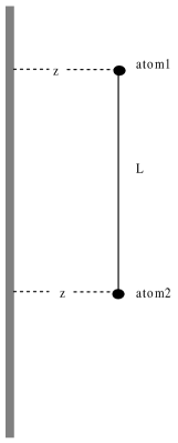
Figure 1: The infinite conducting plate is taken to lie along the plane $z=0$, the distance between each atom and the plate is $z$, the atom separation is $L$

$$G_{ij}^{(11)}(t-t^{\prime})=G_{ij}^{(22)}(t-t^{\prime})= -{1\over 4\pi^{2}}\sum_{m=-\infty}^{\infty}\bigg{[}{\delta_{ij}\over(t-t^{\prime}-im\beta-i\epsilon)^{2}}$$ (15)

$$-{\delta_{ij}\over(t-t^{\prime}-im\beta-i\epsilon)^{2}-(2z)^{2}}\bigg{]}\;,$$

$$G_{ij}^{(21)}(t-t^{\prime})=G_{ij}^{(12)}(t-t^{\prime})= -{1\over 4\pi^{2}}\sum_{m=-\infty}^{\infty}\bigg{[}{\delta_{ij}\over(t-t^{\prime}-im\beta-i\epsilon)^{2}-L^{2}}$$ (16)

$$-{\delta_{ij}\over(t-t^{\prime}-im\beta-i\epsilon)^{2}-(2z)^{2}-L^{2}}\bigg{]}\;,$$

where $\beta=1/(kT)$. Plugging Eq. (15) and Eq. (16) into the Eq. (9), we can easily obtain

$${\cal G}^{(11)}_{ij}(\lambda)={\cal G}^{(22)}_{ij}(\lambda)=\frac{\delta_{ij}}{2\pi}\frac{\lambda}{1-e^{-\beta\lambda}}-\frac{\delta_{ij}}{2\pi}\frac{\lambda}{1-e^{-\beta\lambda}}\frac{\sin(2z\lambda)}{2z\lambda},$$

$${\cal G}^{(12)}_{ij}(\lambda)={\cal G}^{(21)}_{ij}(\lambda)=\frac{\delta_{ij}}{2\pi}\frac{\lambda}{1-e^{-\beta\lambda}}\ \frac{\sin(L\lambda)}{L\lambda}-\frac{\delta_{ij}}{2\pi}\frac{\lambda}{1-e^{-\beta\lambda}}\frac{\sin(\sqrt{L^{2}+4z^{2}}\lambda)}{\sqrt{L^{2}+4z^{2}}\lambda}\;.$$ (17)

According to Eq. (11), we can write

$$C_{ij}^{(11)}=C_{ij}^{(22)}=A_{1}\delta_{ij}-iB_{1}\epsilon_{ijk}n_{k}+C_{1}n_{i}n_{j}$$

$$C_{ij}^{(12)}=C_{ij}^{(21)}=A_{2}\delta_{ij}-iB_{2}\epsilon_{ijk}n_{k}+C_{2}n_{i}n_{j}\;,$$ (18)

and the corresponding coefficients are

$$A_{1}={\omega\over 4\pi}{1+e^{-\beta{\omega}}\over 1-e^{-\beta{\omega}}}\bigg{[}1-{\sin(2z\omega)\over 2z\omega}\bigg{]}\;,\hskip 10.0ptA_{2}={\omega\over 4\pi}{1+e^{-\beta{\omega}}\over 1-e^{-\beta{\omega}}}\bigg{[}{\sin(L\omega)\over{L\omega}}-{\sin(\sqrt{L^{2}+4z^{2}}\omega)\over\sqrt{L^{2}+4z^{2}}\omega}\bigg{]}\;,$$

$$B_{1}={\omega\over 4\pi}\bigg{[}1-{\sin(2z\omega)\over 2z\omega}\bigg{]}\;,\hskip 50.0ptB_{2}={\omega\over 4\pi}\bigg{[}{\sin(L\omega)\over{L\omega}}-{\sin(\sqrt{L^{2}+4z^{2}}\omega)\over\sqrt{L^{2}+4z^{2}}\omega}\bigg{]}\;,$$

$$C_{1}={\omega\over 4\pi}{1+e^{-\beta{\omega}}\over 1-e^{-\beta{\omega}}}\bigg{[}-1+{\sin(2z\omega)\over 2z\omega}\bigg{]}\;,$$

$$C_{2}={\omega\over 4\pi}{1+e^{-\beta{\omega}}\over 1-e^{-\beta{\omega}}}\bigg{[}-{\sin(L\omega)\over{L\omega}}+{\sin(\sqrt{L^{2}+4z^{2}}\omega)\over\sqrt{L^{2}+4z^{2}}\omega}\bigg{]}\;.$$ (19)

Similarly, the ${\cal K}_{ij}^{\alpha\beta}$ for the Hamiltonian $H_{\rm eff}$ can be obtained easily, but here we do not give the formulae in detail. As has already been discussed in detail elsewhere Benatti1 ; Benatti2 , the effective Hamiltonian $H_{\rm eff}$ can be expressed as a sum of three pieces. The first two correspond to the corrections of the Lamb shift at a finite temperature which should be regularized according to the standard procedures in quantum field theory and nevertheless they can be accounted for by replacing $\omega$ in the atom’s Hamiltonian $H_{S}$ with a renormalized energy level spacing

$$\tilde{\omega}=\omega+i[{\cal K}^{11}(-\omega)-{\cal K}^{11}(\omega)]\;.$$ (20)

Meanwhile the third is an environment generated direct coupling between the atoms and it is temperature independent. So the term associated with $H_{\rm eff}$ in (5) can be ignored, since we are interested in the temperature-induced effects. Henceforth, we will only study the effects produced by the dissipative part ${\cal L}[\rho(t)]$.

Using the explicit form of the master equation (5), we can investigate the time evolution of the reduced density matrix and figure out whether the state of the two-level atom system is an entangled one or not with the help of partial transposition criterion ppt : a two-atom state $\rho(t)$ is entangled at $t$ if and only if the operation of partial transposition of $\rho(t)$ does not preserve its positivity. In general, the two-atom system in the thermal bath will be subjected to decoherence and dissipation, which may counteract the entanglement production, so that the final equilibrium state is very likely to be separable (however this may not always be true as we will demonstrate later). But if we consider the system evolving in a finite time, during which the decoherence and dissipation are not dominant, the initial separable state may evolve to an entangled one. Here, we adopt a simple strategy for ascertaining the entanglement creation at a neighborhood of the initial time $t=0$, which has been introduced in Ref. pr5 . For simplicity, we let the initial pure, separable two-atom state be $\rho(0)=|+\rangle\langle+|\otimes|-\rangle\langle-|$ and consider the quantity

$${\cal Q}(t)=\langle\chi|\,\tilde{\rho}(t)\,|\chi\rangle\ ,$$ (21)

where the tilde signifies partial transposition and $|\chi\rangle$ is a properly chosen $4$-dimensional vector. According to the results of Ref. Benatti2 ; pr5 ), entanglement is created at the neighborhood of time $t=0$ (i.e., $\partial_{t}{\cal Q}(0)<0$), if and only if

$$\langle{u}|C^{(11)}|u\rangle\langle{v}|(C^{(22)})^{T})|v\rangle<|\langle{u}|Re(C^{(12)})|v\rangle|^{2}\;,$$ (22)

where the subscript $T$ means matrix transposition and the three-dimensional vectors $|u\rangle$ and $|v\rangle$ can be chosen in a simple form as $u_{i}=v_{i}=\{1,-i,0\}$. Using Eq. (19), we can calculate Eq. (22) for the vector $\mathbf{n}$ along the third axis directly and deduce that the condition (22) becomes

$$\bigg{(}{A_{2}\over{A_{1}}}\bigg{)}^{2}+\bigg{(}{B_{1}\over{A_{1}}}\bigg{)}^{2}>1\;,$$ (23)

where

$$\bigg{(}{B_{1}\over{A_{1}}}\bigg{)}^{2}=\bigg{(}{1-e^{-\beta{\omega}}\over 1+e^{-\beta{\omega}}}\bigg{)}^{2}\;,$$ (24)

$$\bigg{(}{A_{2}\over{A_{1}}}\bigg{)}^{2} = \bigg{(}{\sin(L\omega)\over{L\omega}}-{\sin(\omega\sqrt{L^{2}+4z^{2}})\over{\omega\sqrt{L^{2}+4z^{2}}}}\bigg{)}^{2}/\bigg{(}1-{\sin(2\omega{z})\over 2z{\omega}}\bigg{)}^{2}\;.$$ (25)

For a given energy gap for the atoms, ${B_{1}}^{2}/{A_{1}}^{2}$ takes the values in the interval [ 0, 1 ] and is only temperature-dependent, while the value of ${A_{2}}^{2}/{A_{1}}^{2}$ is determined by two parameters, $z$ and $L$ and is temperature independent. One can see that when the temperature is zero i.e. $\beta\rightarrow\infty$ and $L$ is not infinite, the inequality (23) is always satisfied, therefore entanglement is generated. At the same time, if the separation is vanishing ($L=0$), then ${A_{2}}^{2}/{A_{1}}^{2}$ becomes unity and the inequality (23) is always obeyed and thus entanglement created too, no matter where the atoms are placed, as long as the bath temperature is not infinite.

Let us now discuss what happens when $z\rightarrow 0$ or $z\ll L$, and $z\rightarrow\infty$ or $z\gg L$, i.e., when the atoms are placed very close to and very far from the boundary. Expansion of Eq. (25) in power series of $z/L$ yields

$$\bigg{(}{A_{2}\over{A_{1}}}\bigg{)}^{2} \approx \frac{9}{\omega^{6}L^{6}}\bigg{[}-\omega{L}\cos(\omega{L})+\sin(\omega{L})\bigg{]}^{2}+\frac{18}{5\omega^{6}L^{6}}\bigg{[}\omega{L}\cos(\omega{L})-\sin(\omega{L})\bigg{]}\times$$ (26)

$$\quad\bigg{[}\omega{L}(-15+\omega^{2}L^{2})\cos(\omega{L})+3(5-2\omega^{2}L^{2})\sin(\omega{L})\bigg{]}\bigg{(}{z\over L}\bigg{)}^{2}\;.$$

The corresponding form for $z/L\rightarrow\infty$ reads

$$\bigg{(}{A_{2}\over{A_{1}}}\bigg{)}^{2}\approx\frac{\sin^{2}(\omega{L})}{\omega^{2}L^{2}}+\frac{L}{z}\frac{\sin(\omega{L})}{\omega^{3}L^{3}}\bigg{[}\sin(\omega{L})\sin(2{\omega}z)-\omega{L}\sin(\omega{L}\sqrt{1+4z^{2}/L^{2}})\bigg{]}\;,$$ (27)

where ${\sin^{2}(\omega{L})}/{\omega^{2}L^{2}}$ is just the value of ${A_{2}}^{2}/{A_{1}}^{2}$ without the presence of the boundary Benatti2 (i.e., the corresponding value of ${A_{2}}^{2}/{A_{1}}^{2}$ in the limit of $z\rightarrow\infty$). It is interesting to note that in the limit of $z/L\rightarrow 0$, the leading term of ${A_{2}}^{2}/{A_{1}}^{2}$ is independent on $z$ and is only a function of $\omega L$ (refer to Eq. (26)). This leading term differs from the value of ${A_{2}}^{2}/{A_{1}}^{2}$ in the case without the boundary. As a result, when the atoms are placed very close to the boundary, the presence of the boundary will have a significant effect in determining whether the inequality (23) is satisfied or whether entanglement is created. In Fig. (2), the leading term of ${A_{2}}^{2}/{A_{1}}^{2}$ when $z/L\rightarrow 0$ is plotted as a function of $\omega{L}$ vs ${A_{2}}^{2}/{A_{1}}^{2}$ in the case without the boundary. This Figure reveals that when $\omega{L}$ is small, approximately smaller than 3, that is when the separation, $L$, is approximately less than three times the characteristic wavelength of the atom’s radiation (but L is still large enough to maintain $z\ll L$), the value of ${A_{2}}^{2}/{A_{1}}^{2}$ in the case with the presence of a boundary will be appreciably larger than that without as long as $L$ is not vanishingly small. This means that at a certain temperature the presence of a boundary would make the atoms be entangled which otherwise still be separable. Therefore the presence of the boundary provides us more freedom in controlling entanglement creation in this case. However, when $\omega{L}$ is large, i.e., the separation is much larger than the characteristic wavelength of the atom’s radiation, the value of ${A_{2}}^{2}/{A_{1}}^{2}$ with the presence of the boundary generally becomes smaller than that without, since it decreases faster (as power of $(\omega{L})^{-6}$ as opposed to $(\omega{L})^{-2}$) as $\omega{L}$ grows. Therefore, in this case the presence of the boundary will make the atoms less likely to be entangled than otherwise. Meanwhile when $z/L$ is very large, i.e., when the atoms are very far from the boundary, the influence of the presence of the boundary on the entanglement generation is negligible as expected and this can be easily seen from Eq. (27) since now the leading term is the same as the value of ${A_{2}}^{2}/{A_{1}}^{2}$ in the unbounded case.

Figure 2: The dashed line represents $A_{2}^{2}/A_{1}^{2}$ in the limit of $z/L\rightarrow 0$, and the solid line denotes the function, $\sin^{2}(\omega{L})/(\omega{L})^{2}$, i.e, $A_{2}^{2}/A_{1}^{2}$ without presence of a boundary. Approximately in the interval [0,3] of $\omega{L}$, the value of ${A_{2}}^{2}/{A_{1}}^{2}$ with the presence of the boundary is always larger than that without.

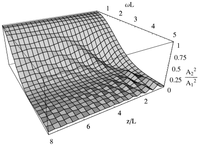
Figure 3: ${A_{2}}^{2}/{A_{1}}^{2}$ as a function of two dimensionless variables, $z/L$ and $\omega{L}$.

To have a better understanding, we also plot, in Fig. (3), ${A_{2}}^{2}/{A_{1}}^{2}$ as a function of two dimensionless variables, $z/L$ and $\omega{L}$, according to Eq. (25). One can see from this figure that, as $z/L$ varies, appreciable oscillations occur when $\omega{L}$ is of order one and when $\omega{L}$ is very small, the value of ${A_{2}}^{2}/{A_{1}}^{2}$ is very close to unity and does not oscillate significantly as $z/L$ varies. At same time, ${A_{2}}^{2}/{A_{1}}^{2}$ also decays very fast with the increase of $\omega{L}$ and the oscillations (as $z/L$ varies) is damped dramatically. So we conclude that both when $\omega{L}$ is very small or very large, the variation of location of the atoms has no significant influence on the entanglement generation. Note, however, that this by no means suggests that the presence of the boundary does not affect the entanglement generation (refer to the discussions in the preceding paragraph).

The next question we want to ask is what is the maximum difference between the value of ${A_{2}}^{2}/{A_{1}}^{2}$ with the presence of a boundary and that without. We will try to answer the question numerically and approximately.

Figure 4: The ratio ${A_{2}}^{2}/{A_{1}}^{2}$ is described as a function of the $z/L$ in the real line, with the parameter are selected $\omega{L}=(0.5,1,1.5,2.027,2.8)$. The dashing line expresses the value of $\sin^{2}(\omega{L})/(\omega{L})^{2}$ which is the value of ${A_{2}}^{2}/{A_{1}}^{2}$ without the boundary conditions. As we can easily see that all the values of ${A_{2}}^{2}/{A_{1}}^{2}$ vibrate around the $\sin^{2}(\omega{L})/(\omega{L})^{2}$.

For this purpose, let us plot, in Fig. (4), ${A_{2}}^{2}/{A_{1}}^{2}$ as a function of $z/L$ with a set of fixed values of the dimensionless parameter $\omega{L}$ in both the cases with and without a boundary. Our numerical calculations as shown illustratively in Fig. (4) indicate that the maximum fluctuation of ${A_{2}}^{2}/{A_{1}}^{2}$ in the case with the presence of the boundary around that without as a function of $z/L$ is at the neighborhood of $\omega{L}\approx 2.027$. Setting $\omega{L}\approx 2.027$, we find that the function of ${A_{2}}^{2}/{A_{1}}^{2}$ vibrates around $\sin^{2}(\omega{L})/(\omega{L})^{2}\approx 0.196$. Due to the fact that the swing of vibrating function ${A_{2}}^{2}/{A_{1}}^{2}$ is slowly decreasing with the increasing $z/L$, we can find out the maximum value of ${A_{2}}^{2}/{A_{1}}^{2}$, by adjusting the parameter $z/L$, to be approximately $0.416$ achieved at $z/L\ll 1$. This gives the maximum effects of the presence of the boundary on ${A_{2}}^{2}/{A_{1}}^{2}$ or equivalently on entanglement creation.

To get a more concrete picture, let us take a typical transition frequency of a hydrogen atom, $\omega\sim 10^{14}Hz$, for an example. Then $\omega{L}\approx 2.027$ means $L\approx 6.08\times 10^{-6}m$ which is much larger than the usual size of an atom. It is easy to find that in the unbounded space the inequality (23) is satisfied or entanglement is created between two atoms if the temperature is below $262.663$K. However, with the presence of a boundary, we find that the upper bound in temperature for entanglement generation can be increased to $T<379.731$K. This is a hundred Kelvins improvement. Note for $L\approx 6.08\times 10^{-6}m$, we still have a plenty of room to satisfy $z/L\ll 1$, so the maximum value of $0.416$ is used for ${A_{2}}^{2}/{A_{1}}^{2}$ here.

Finally, let us briefly discuss what happens if the two-atom system is not aligned strictly parallel to the plane boundary. Take the distance from the plane of the atom which is closer as $z$, then the distance of the other atom from the plane will be be larger or smaller than $z$ depending on whether the system is inclined away from or towards the boundary. Therefore the effect of inclination of the system is that the field correlation function with respect to the atom which is displaced and cross correlation function $G_{ij}^{(21)}(t-t^{\prime})=G_{ij}^{(12)}(t-t^{\prime})$ effectively get a smaller effective $z$ if the system is inclined towards the plane and a larger effective one if otherwise (refer to Eqs. (15,16)). Consequently, taking into account the fact that ${A_{2}}^{2}/{A_{1}}^{2}$ is an oscillating function of $z$ when the system is parallelly placed, one would expect that if the two atom system is originally located parallel to the plane at where this function is at its peak value the inclination in either direction will make the entanglement creation less likely to occur. In contrast, if the system is located at where this function is at its local minimum the inclination in either direction will make the entanglement generation more likely to happen. However, when the system is placed at any point in the interval where function ${A_{2}}^{2}/{A_{1}}^{2}$ is monotonically increasing, the atoms will be less likely to entangle if the inclination is towards the plane and more likely if otherwise. Similarly, when the system is located at any point in the interval where function ${A_{2}}^{2}/{A_{1}}^{2}$ is monotonically decreasing, the entanglement generation will be more likely to come about if the inclination is towards the plane and less likely if otherwise.

IV The entanglement of the equilibrium state with the boundary

In the preceding Section, we find that, in certain circumstances, the presence of a boundary plays a significant role in generating entanglement between atoms initially prepared in a separable state in a thermal bath of external quantum scalar fields and in fact entanglement is created as soon as time starts if the inequality (23) is satisfied. However, the condition (23) does not tell us whether the entanglement thus generated can persist in late times, or whether the final equilibrium state is still entangled or not.

At late times, the two-atom subsystem will be in the asymptotic equilibrium state. Though the effects of decoherence and dissipation will generically make the state be separable so that no entanglement is left in the end, there are also cases in which the entanglement still exists at late times. To examine whether the final equilibrium state is entangled or not, let us assume, without loss of generality, the reduced density matrix to have the form

$$\rho(t)={1\over 4}\bigg{[}\sigma_{0}\otimes\sigma_{0}+\rho_{0i}(t)\;\sigma_{0}\otimes\sigma_{i}+\rho_{i0}(t)\sigma_{i}\otimes\sigma_{0}+\rho_{ij}(t)\sigma_{i}\otimes\sigma_{j}\bigg{]}\;,$$ (28)

where the components $\rho_{0i}(t),\rho_{i0}(t),\rho_{ij}(t)$ are real. Substituting Eq. (28) into Eq. (5), we can obtain, with setting $H_{\rm eff}=0$,

$${\partial{\rho_{0i}(t)}\over\partial{t}}=-4A_{1}\rho_{0i}(t)-4B_{1}n_{i}-2B_{2}n_{i}\tau+2B_{2}n_{k}\rho_{ik}(t)-2C_{1}\rho_{0i}(t)+2C_{1}n_{i}n_{k}\rho_{0k}(t)\;,$$ (29)

$${\partial{\rho_{i0}(t)}\over\partial{t}}=-4A_{1}\rho_{i0}(t)-4B_{1}n_{i}-2B_{2}n_{i}\tau+2B_{2}n_{k}\rho_{ki}(t)-2C_{1}\rho_{i0}(t)+2C_{1}n_{i}n_{k}\rho_{k0}(t)\;,$$ (30)

$${\partial{\rho_{ij}(t)}\over\partial{t}} = -8A_{1}\rho_{ij}(t)-4A_{2}\rho_{ji}(t)+4A_{2}\tau\delta_{ij}-4B_{1}[n_{i}\rho_{0j}(t)+n_{j}\rho_{i0}(t)]$$ (31)

$$-2B_{2}[n_{i}\rho_{j0}(t)+n_{j}\rho_{0i}(t)]+2B_{2}[n_{k}(\rho_{k0}(t)+\rho_{0k}(t))]\delta_{ij}$$

$$-4C_{1}\rho_{ij}(t)-4C_{2}\rho_{ji}(t)+4C_{2}[n_{i}n_{k}\rho_{jk}(t)+n_{j}n_{k}\rho_{ki}(t)-n_{i}n_{j}\tau]$$

$$+2C_{1}[n_{i}n_{k}\rho_{kj}(t)+n_{j}n_{k}\rho_{ik}(t)]+4C_{2}[\tau-n_{k}n_{l}\rho_{kl}(t)]\delta_{ij}\;.$$

Here, $\tau$ is the trace of the density matrix $\tau=\Sigma_{i=1}^{3}\rho_{ii}(t)$. Recall that $n_{i}$ are the components of the unit vector appearing, for example, in Eq. (2) and Eq. (12). If we symmetrize and anti-symmetrize the density matrix components $\rho_{oi}(t),\;\rho_{ij}(t)$, we can split the above system of differential equations into two independent sets. One can then show that the anti-symmetrized components decay exponentially as time grows while the symmetrized ones approach a non-zero asymptotic value. Therefore, there exists a final equilibrium state $\hat{\rho}$, the explicit form of which, for a non-zero atom separation, can be found by setting the right hand side of Eq. (29), Eq. (30), and Eq. (31) to be zero, since any equilibrium state satisfies $\partial_{t}\hat{\rho}=0$, and the solution is

$$\tau={(2A_{1}+A_{2})B_{1}(B_{1}-B_{2})\over 2{A_{1}}^{3}-{A_{1}}^{2}A_{2}-A_{2}B_{1}B_{2}+A_{1}({B_{2}}^{2}-{A_{2}}^{2})}$$

$$\hat{\rho}_{0i}=\hat{\rho}_{i0}=-{({A_{1}-A_{2}})B_{1}(2A_{1}+A_{2})n_{i}\over 2{A_{1}}^{3}-{A_{1}}^{2}A_{2}-A_{2}B_{1}B_{2}+A_{1}({B_{2}}^{2}-{A_{2}}^{2})}\;,$$

$$\hat{\rho}_{ij}={({A_{1}-A_{2}})B_{1}(2B_{1}+B_{2})n_{i}n_{j}\over 2{A_{1}}^{3}-{A_{1}}^{2}A_{2}-A_{2}B_{1}B_{2}+A_{1}({B_{2}}^{2}-{A_{2}}^{2})}\;.$$ (32)

To see if the equilibrium state is entangled or not, we will calculate its concurrence which is defined to be ${\cal C}[\rho]=\max\{\lambda_{1}-\lambda_{2}-\lambda_{3}-\lambda_{4}\}\;$, where $\lambda_{\mu}\;,\mu=1,2,3,4\;$, are the square roots of the non-negative eigenvalues of the matrix $\rho\widetilde{\rho}$ in decreasing order. Here, the auxiliary matrix $\widetilde{\rho}=(\sigma_{2}\otimes\sigma_{2})\rho^{T}(\sigma_{2}\otimes\sigma_{2})\;$. Substituting Eq. (IV) into Eq. (28), we can easily calculate the concurrence for the unit vector $\mathbf{{n}}$ along the third axis via the above the equations. It is found that the concurrence is zero, which means that the equilibrium state is separable and entanglement generated initially does not persist at late times. Same results can be obtained for ${\bf{n}}$ along other directions.

However, it should be pointed out that all the expressions of Eq. (IV) become indefinite (of the form $0/0$) when the separation of the atom approaches zero which results in $A_{1}=A_{2},B_{1}=B_{2},C_{1}=C_{2}$. Therefore, the case for the vanishing atom separation should be dealt with separately. Taking the trace of both sides of Eq. (31) for the vanishing atom separation, we find that $\tau=\Sigma_{i=1}^{3}\rho_{ii}(t)$ is actually a constant of motion, which is determined by the initial reduced density, while the expression for $\tau$ in Eq. (IV) is no longer valid. In fact, the positivity of the initial density matrix requires that $-3\leq\tau\leq 1$. Consequently, we should take $\tau$ as a new independent parameter, and components of the density matrix for the equilibrium state, $\hat{\rho}$, in the present case, read

$$\hat{\rho}_{0i}=\hat{\rho}_{i0}=-{R\over 3+R^{2}}(\tau+3)n_{i}\;,$$

$$\hat{\rho}_{ij}={1\over 3+R^{2}}[(\tau-R^{2})\delta_{ij}+R^{2}(\tau+3)n_{i}n_{j}]\,,$$ (33)

where $R=B_{1}/A_{1}$. The corresponding concurrence can be calculated directly

$${\cal C}(\hat{\rho})=\max\Bigg{\{}{(3-R^{2})\over 2(3+R^{2})}\bigg{[}{5R^{2}-3\over 3-R^{2}}-\tau\bigg{]},0\Bigg{\}}\;,$$ (34)

which is non-zero provided $\tau$ for the initial state $\rho(0)$ obeys

$$\tau<{5R^{2}-3\over 3-R^{2}}\;.$$ (35)

This reveals that when the atom separation is zero ($L=0$), the entanglement generated initially persists at late time despite of the decoherence and dissipation of the external environment and the late-time equilibrium state is still entangled, as long as (35) holds. This is in sharp contrast with the case of a non-zero separation. However, the presence of the boundary has on effect on deciding whether the initially created entanglement can be maintained at late times in the equilibrium state, since the concurrence is only dependent on $\tau$ and $R$, and factors containing the boundary parameter $z$ are all canceled out in the expression of $R$ if one recalls Eq. (19), thus the concurrence for the final equilibrium state is independent of the presence boundary.

V Discussion

In summary, we have examined the entanglement generation between two mutually independent two-level atoms immersed in a thermal bath of scalar particles subjected to a perfectly reflecting plane boundary. With the help of the master equation that describes the evolution in time of the atom subsystem obtained by tracing over environment (external scalar fields) degrees of freedom, we find that the presence of the boundary may play a significant role in controlling the entanglement creation in some circumstances and the new parameter, the distance of the atoms from the boundary, gives one more freedom in controlling the entanglement generation.

In particular, when two atoms are placed very close to the boundary, i.e., $z/L\ll 1$ and $\omega L$ is approximately less than three, that is, when the separation, $L$, is approximately less than three times the characteristic wavelength of the atom’s radiation, then for a certain temperature the presence of the boundary will make the atoms be entangled which would otherwise still be separable. Therefore the presence of the boundary gives us more power in creating entanglement. However, when $\omega{L}$ is large, i.e., the separation is much larger than the characteristic wavelength of the atom’s radiation, the presence of the boundary will make the atoms less likely to be entangled than otherwise. Meanwhile when $z/L$ is very large, i.e., when the atoms are very far from the boundary, the influence of the presence of the boundary on the entanglement generation is negligible as expected.

At the same time, we find that the variation of location of the atoms has significant influence on entanglement generation between two initially independent atom only when $\omega{L}$ is of order one, or in different words, both when $\omega{L}$ is very small or very large, the variation of location of the atoms has no appreciable effect on the entanglement generation. Note, however, that this by no means suggests that the presence of the boundary does not affect the entanglement generation.

Our analysis also reveals that the entanglement generated because of the correlations induced by the environment will persist in the late time asymptotic equilibrium state if the separation between the atoms is vanishing. However, when the separation is non-zero, the entanglement will disappear at late times and the asymptotic equilibrium state becomes unentangled again. Finally, the presence of a boundary generally has no effect on maintaining the entanglement initially generated in the asymptotic equilibrium state.

- (1) M. B. Plenio and V. Vedral, Contemp. Phys. 39, 431 (1998); B. Schumacher and M. D. Westmoreland, quant-ph/0004045; M. Horodecki, Quant. Inf. Comp. 1, 3 (2001); P. Horodecki and R. Horodecki, Quant. Inf. Comp.1, 45 (2001); J. Eisert and M. B. Plenio, Int. J. Quant. Inf. 1, 479 (2003).
- (2) C. H. Bennett and S.J. Wiesner, Phys. Rev. Lett. 69, 2881 (1992); C. H. Bennett, P. W. Shor, J. A. Smolin and A.V. Thapliyal, Phys. Rev. Lett. 83, 3081-3084 (1999).
- (3) C. H. Bennett, G. Brassard, C. Cr epeau, R. Jozsa, A. Peres, W. K. Wootters, Phys. Rev. Lett. 70, 1895 (1993).
- (4) A. K. Ekert, Phys. Rev. Lett. 67, 661-663 (1991).
- (5) D. Braun, Phys. Rev. Lett. 89 277901 (2002).
- (6) M. S. Kim, J. Lee, D. Ahn and P. L. Knight, Phys. Rev. A 65 040101(R) (2002).
- (7) L. Jakobczyk, J. Phys. A 35 6383 (2002).
- (8) S. Schneider and G.J. Milburn, Phys. Rev. A 65 042107 (2002).
- (9) F. Benatti, R. Floreanini and M. Piani, Phys. Rev. Lett. 91 070402 (2003).
- (10) A. M. Basharov, J. Exp. Theor. Phys. 94, 1070 (2002).
- (11) F. Benatti and R. Floreanini , Phys. Rev. A. 70 012112 (2004).
- (12) F. Benatti and R. Floreanini, J. Opt. B. 7, S429 (2005).
- (13) H. B. G. Casimir, Proc.K.Ned.Akad.Wet. 51, 793 (1948).
- (14) H. Yu and L. H. Ford, Phys. Rev. D 60, 084023 (1999); H. Yu and L. H. Ford, Phys. Lett. B 496, 107 (2000); H. Yu and P. X. Wu, Phys. Rev. D 68, 084019 (2003).
- (15) H. Yu and L. H. Ford, Phys. Rev. D 70, 065009 (2004); H. Yu and J. Chen, Phys. Rev. D 70 125006 (2004).
- (16) H. Yu and S. Lu Phys. Rev. D 72 064022 (2005); H. Yu and Z. Zhu, Phys. Rev. D 74, 044032 (2006).
- (17) V. Gorini, A. Kossakowski, and E. C. G. Surdarshan, J. Math. Phys. 17, 821 (1976); G. Lindblad, Commun. Math. Phys. 48, 119 (1976).
- (18) N. D. Birrell and P. C. W. Davies 1987 Quantum Fields in Curved Space (Cambridge: Cambridge University Press) Chap 4.
- (19) A. Peres, Phys. Rev. Lett. 77 1413 (1996); M. Horodecki, P. Horodecki and R. Horodecki, Phys. Lett. A 233, 1(1996).