Entanglement and optimal strings of qubits for memory channels
V. Karimipour          L. Memarzadeh,

Department of Physics,

Sharif University of Technology,

P.O. Box 11365-9161,

Tehran, Iran

We investigate the problem of enhancement of mutual information by encoding classical data into entangled input states of arbitrary length and show that while there is a threshold memory or correlation parameter beyond which entangled states outperform the separable states, resulting in a higher mutual information, this memory threshold increases toward unity as the length of the string increases. These observations imply that encoding classical data into entangled states may not enhance the classical capacity of quantum channels.

PACS Numbers: 03.67.-a, 03.67.Hk

1 Introduction

Consider a quantum channel defined by a completely positive trace preserving map $\rho\longrightarrow\mathcal{E}^{(1)}(\rho)$. We use ${\mathcal{E}}^{(1)}$ for describing the action of the channel on one qubit and ${\mathcal{E}}^{(n)}$ for its action on a string of qubits of length $n$. By encoding classical data into quantum states and performing optimal measurements at the output, such a channel can be used for communicating classical information. One is then faced with the natural question of which states are the optimal ones for encoding the input data, that is, which ensemble of input states maximize the mutual information between the sender and the receiver.

If the input strings are disentangled and if consecutive uses of the channel are not correlated to each other, that is for memoryless channels, then the action of the channel on a string $\rho_{1}\otimes\rho_{2}\cdots\otimes\rho_{n}$ is simple, namely it is given by ${\mathcal{E}}^{n}(\rho_{1}\otimes\rho_{2}\cdots\otimes\rho_{n})=\bigotimes_{i=1}^{n}{\mathcal{E}}^{1}(\rho_{i})$. However in general one may want to encode classical data into entangled strings or, consecutive uses of the channel may be correlated to each other, in which case ${\mathcal{E}}^{n}\neq{{\mathcal{E}}^{1}}^{\otimes n}$. In these cases the output strings are no longer simple functions of the input strings.

In these cases we are dealing with a strongly correlated quantum system the correlations of which either result from the entanglements of the input states, or from the memory of the channel itself. And for this reason we should anticipate grave difficulties in analytical tackling of the problem. Nevertheless we try to gain an insight by studying examples.

Given an ensemble of input states $\varepsilon:=\{\rho_{i},p_{i}\}$ where $p_{i}$ are the probabilities of states $\rho_{i}$, and $\rho_{i}$ are states of $n-$ input qubits, the mutual information is defined as

$$I_{n}(\varepsilon):=S({\mathcal{E}}^{(n)}(\sum_{i}p_{i}\rho_{i}))-\sum_{i}p_{i}S({\mathcal{E}}^{n}(\rho_{i})),$$ (1)

where $S(\rho)\equiv-tr(\rho\log\rho)$ is the von Neumann entropy of a state $\rho$.

A basic question of information theory is whether there is any advantage in using entangled states as input states, that is, whether or not encoding the classical data into entangled rather than separable states increases the mutual information. For the case when multiple uses of the channel are not correlated, there are partial evidence based on studying concrete examples [1], [2], [3]that the optimal states are separable and hence there is no advantage in using entangled states.

However if multiple uses of the channel are correlated, then there are pieces of evidence that entangled states become advantageous, once the correlation exceeds a critical value.

In [4, 5] a Pauli channel with partial memory, was studied. The action of the channel on two consecutive qubits is given by the following map:

$${\mathcal{E}}(\rho)=\sum_{i,j}P_{ij}(\sigma_{i}\otimes\sigma_{j})\rho(\sigma_{i}\otimes\sigma_{j})^{{\dagger}},$$ (2)

where $P_{ij}$ denotes the probability of two consecutive errors $\sigma_{i},\sigma_{j}$ and is defined as:

$$P_{ij}=(1-\mu)p_{i}p_{j}+\mu\delta_{i,j}p_{i}=[(1-\mu)p_{i}+\mu\delta_{i,j}]p_{j}.$$ (3)

Here $p_{i}$ is the probability of the error operator $\sigma_{i}$, $i=0,1,2,3$ on one single qubit. Thus with probability $\mu$ the channel acts on the second qubit with the same error operator as on the first qubit, and with probability $(1-\mu)$ it acts on the second qubit independently, hence the name partial memory.

Physically the parameter $\mu$ is determined by the relaxation time of the channel when a qubit passes through it. In order to remove correlations, one can wait until the channel has relaxed to its original state before sending the next qubit, however this lowers the rate of information transfer. Thus it is necessary to consider the performance of the channel for arbitrary values of $\mu$ to reach a compromise between various factors which determine the final rate of information transfer.

In [4] it was shown by analytical arguments and numerical searches in the space of two-qubit input states, that for the depolarizing channel [6] there is a sharp transition in the type of optimal states from separable to maximally entangled states when the memory parameter $\mu$ passes beyond a critical value $\mu_{c}$. A similar result was established analytically by the same authors in [5] who considered a particularly symmetric channel with ($p_{0}=p_{3}$ and $p_{1}=p_{2}$). Inspired by these works, similar results have been shown for generalized Pauli channels acting on states of arbitrary dimensions or qudits in [7, 8] and for bosonic Gaussian channels in [9].

However all the above studies have been restricted to strings of states of length $n=2$. As is well known from theorems on data compression in classical [10] and quantum [11] information theory, one should encode classical data into arbitrarily long sequences of bits or qubits. This is quite necessary if one wants to encode with arbitrarily high probability only typical sequences and achieve maximum compression of data and minimum decoding errors.
This requirement is also reflected in the definition of classical capacity of quantum channels which is given by

$$C:=\lim_{n\rightarrow\infty}C_{n}$$ (4)

where

$$C_{n}:=\frac{1}{n}Sup_{\varepsilon}I_{n}(\varepsilon),$$ (5)

in which $n$ is the length of input string of states.

Thus the question of whether entanglement enhances the mutual information or not should be addressed for strings of arbitrary length and not just strings of length $2$. More concretely one may ask if it is advantageous to encode $2^{n}$ bits of information into completely separable states of $n$ qubits or else, into maximally entangled states. Only then one can make precise statements as to the enhancement effect of entanglement on the mutual information and capacity of quantum channels.

We should stress that the answer to this question, whatever it may be, does not invalidate the previous results, that entangled states give a higher mutual information than separable states, as long as we use a correlated channel ”twice”. However if consecutive uses of a channel are correlated, and we have to encode our data into arbitrary long strings, that is we are streaming the data into the channel, then we should consider the effect of this correlation on all the qubits of the strings. Thus we are asking the question of ”which states maximize the mutual information in the space of all states of $n-$ qubits?”

Unfortunately answering this question in its full generality is almost intractable, for at least two reasons. First it is an extremely difficult task to optimize the mutual information over all ensembles of $n$ qubit states, due to the exponentially large number of parameters involved. Second we do not have good measures to characterize various types of entanglement in multi-partite states. For example in contrast to the two-party case in which we have only one class of entangled states, for $n$-parties there are numerous inequivalent classes of entangled states the number of which grows very rapidly with the number of $n$ [12].

Nevertheless we can gain an insight into this problem by comparing only two types of ensembles, namely an ensemble of pure product states and an ensemble of pure maximally entangled states like the Greenberger-Horne-Zeilinger (GHZ) states. We should stress that even in this case we are still faced with a strongly correlated quantum many body system which poses many computational difficulties for its solution.
There are several reasons in favor of this restricted choice. First following the work of [5] we will show in the sequel that the problem of optimizing the mutual information over input ensembles reduces for Pauli channels to finding a single pure state that minimizes the output entropy. Second, previous examples [4, 5, 8, 7] mentioned above show that as we vary the correlation parameter of the channel $\mu$, the optimal input state (which minimizes the output entropy) changes sharply from a separable state to a maximally entangled state and for no value of this parameter a state with an intermediate value of entanglement is optimal (We will elaborate on this point later in the introduction). Finally an analytic calculation of the output entropy which requires diagnolization of a $2^{n}\times 2^{n}$ matrix is impossible for an arbitrary $n-$ qubit pure state containing many parameters.

Now for the elaboration mentioned above: there is not a single class of maximally entangled states for arbitrary $n$. For example for $n=3$ there are two inequivalent classes which can not be transformed to each other by invertible local operations. Lack of knowledge of all these classes for arbitrary $n$ and the particular simplicity of the $GHZ$ states compels us to consider only this class analytically. In order to substantiate our arguments we also consider other types of encoding of input states, like strings of Bell states by numerical means. However due to the exponential growth of the required time, we have been able only to consider strings of a few number of Bell states which again lead to the same result as stated above.

We have presented in figures (5) and (6) the entropy of output states for several other types of encoding for strings of length 3 and 4.
These figures clearly show that for $n=3$ the optimum input state is a separable state and for $n=4$
the minimum output entropy state is separable for small value of correlation and one or the other type of entangled states for high value of correlation. However in all types of encodings the threshold parameter increases with the length of the strings.

Does these results prove conclusively that encoding classical data into entangled states can not enhance the capacity of quantum channels? Certainly no, because we have not made an exhaustive search over the space of all $n-$ party states. Nevertheless our result casts doubt on the previous hope that this type of entanglement, namely encoding classical data into entangled input states, may increase the capacity of quantum channels for transmitting classical data.

The structure of this paper is as follows: In section (2) we consider the Pauli channel with partial memory and calculate its output states when we pass through it a string of $n$-qubit in either separable or GHZ form. In section (3) we diagonalize the output states and find the eigenvalues of the output states in these two cases to calculate the output entropies and find the critical value of memory above which $GHZ$ states take over the separable states in maximizing the mutual information.
In section (4) we consider other types of entangled states for encoding where we restrict ourselves to strings of length $n=3$ and $n=4$.
Finally section (5) concludes the paper with a discussion and summary of the results. Appendix A contains some details of calculations.

2 The passage of a string of qubits through a Pauli channel with partial memory

2.1 Action of the channel

The action of a Pauli channel with partial memory on a string of $n$ qubits is a natural generalization of equation (2). Before considering the general case, it would be helpful to study the simpler case of $n=3$. In this case we have

$${\mathcal{E}}^{(3)}(\rho)=\sum_{ijk}P_{ijk}(\sigma_{i}\otimes\sigma_{j}\otimes\sigma_{k})\rho(\sigma_{i}\otimes\sigma_{j}\otimes\sigma_{k})^{{\dagger}}.$$ (6)

The memory parameter $\mu$ is contained in the probabilities $P_{ijk}$ which determine the probability of the errors $\sigma_{i}\otimes\sigma_{j}\otimes\sigma_{k}$. Recalling that $(1-\mu)$ is the probability of independent errors on two consecutive qubits , and $\mu$ is the probability of identical errors, $P_{ijk}$ can be written as follows:

$$P_{ijk}=[(1-\mu)p_{i}+\mu\delta_{i,j}][(1-\mu)p_{j}+\mu\delta_{j,k}]p_{k}.$$ (7)

A good way to visualize the pattern of errors is via diagrams depicted in figure (1). A dot with a Latin index say $i$ on it represents an error $\sigma_{i}$ which happens with probability $p_{i}$, and a line represent correlation between two consecutive errors which happens with probability $\mu$. Thus the pattern of errors for a string of three qubits is the one shown in figure (1) and is concisely represented in equation (7).

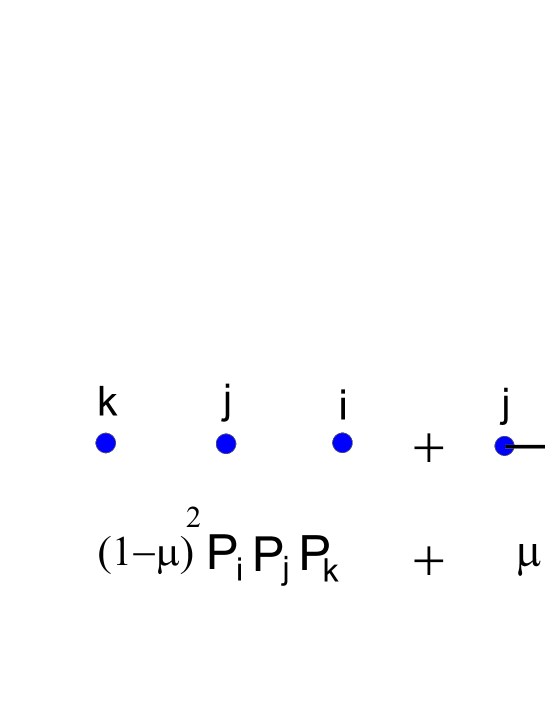
Figure 1: Various types of errors on a string of three qubits and their corresponding graphs. The rightmost graph represents an error which repeats for the second and third bits with probability $\mu^{2}$ and the leftmost graph represents three independent errors.

Note from figure (1) that the sum of probabilities of all types of errors on three qubits adds to unity as we expect:

$$\sum_{i,j,k}\left[(1-\mu)^{2}p_{i}p_{j}p_{k}+2\mu(1-\mu)p_{i}p_{j}+\mu^{2}p_{i}\right]=1.$$ (8)

The action of the channel on a string of $n-$ qubits is given by

$${\mathcal{E}}^{(n)}(\rho)=\sum_{i_{1}\cdots i_{n}=1}^{3}P_{i_{1}\cdots i_{n}}(\sigma_{i_{1}}\otimes\cdots\otimes\sigma_{i_{n}})\rho(\sigma_{i_{1}}\otimes\cdots\otimes\sigma_{i_{n}})^{{\dagger}},$$ (9)

where

$$P_{i_{1}\cdots i_{n}}=p_{i_{n}}\prod_{m=1}^{n-1}\left[(1-\mu)p_{i_{m}}+\mu\delta_{i_{m},i_{m+1}}\right].$$ (10)

Thus in passing through the channel any two consecutive qubits undergo random independent errors with probability $1-\mu$ and identical (correlated) errors with probability $\mu$. This should be the case if the channel has a memory depending on its relaxation time and if we stream the qubits through it.

2.2 Properties of the channel

Since any two Pauli operators either commute or anti-commute with each other, the channel has the following very important property

$${\mathcal{E}}^{(n)}(U\rho U^{{\dagger}})=U{\mathcal{E}}^{(n)}(\rho)U^{{\dagger}},$$ (11)

where $U$ is the $n-$ fold tensor product of any combination of Pauli operators.
Therefore for any state $\rho$ and any operator $U$ of the above form we have

$$S({\mathcal{E}}^{(n)}(U\rho U^{{\dagger}}))=S({\mathcal{E}}^{(n)}(\rho)),$$ (12)

where $S$ is the von-Neumann entropy.

Following the arguments of [5], we now see that the mutual information is saturated by an equiprobable ensemble of the form

$$\varepsilon=\{\rho_{i_{1},i_{2},\cdots i_{n}}:=(\sigma_{i_{1}}\otimes\cdots\sigma_{i_{n}})\rho^{*}(\sigma_{i_{1}}\otimes\cdots\sigma_{i_{n}})^{{\dagger}}\},$$ (13)

where $\rho^{*}$ is the state which minimizes the output entropy. The reason is that the state $\sum_{i_{1},i_{2},\cdots i_{N}}\rho_{i_{1},i_{2},\cdots i_{N}}$ commutes with all the irreducible representation of the Pauli group on $n$ qubits and hence is proportional to the identity. Thus for an equiprobable ensemble of the above type, the first term of (1) is maximized while the second term is minimized due to the minimum output entropy of $\rho^{*}$.
In this way an upper bound for the mutual information is obtained, namely

$$I_{n}({\mathcal{E}}^{(n)})\leq n-S({\mathcal{E}}^{(n)}(\rho^{*})).$$ (14)

Thus the problem of finding the optimal ensemble for maximizing the mutual information reduces to finding the single state $\rho^{*}$ which minimizes the output entropy. Moreover this state can be taken to be a pure state. To see this we again repeat the argument of [5] for completeness: any state $\rho^{*}$ has a decomposition into pure states given by $\rho^{*}=\sum_{i}p_{i}|\Psi_{i}\rangle\langle\Psi_{i}|$. Concavity of $S$ entails that

$$S(\rho^{*})\geq\sum_{i}p_{i}S(|\Psi_{i}\rangle)>S(|\Psi^{*}\rangle),$$

where $|\Psi^{*}\rangle$ is the state with minimal entropy in the decomposition. However by definition of $\rho^{*}$ as the state with minimum entropy we should have $\rho^{*}=|\Psi^{*}\rangle\langle\Psi^{*}|$. This completes the proof that we should only search for a single state to find the optimal ensemble.

2.3 The output states of the channel

2.3.1 Strings of length $n=3$

For simplicity let us first consider strings of length $n=3$. We consider a specific type of symmetric Pauli channel, one for which $p_{0}=p_{3}=p$ and $p_{1}=p_{2}=q$, with $p+q=\frac{1}{2}$. This type of channel was first considered in [5] (for two-qubit strings) for which analytical calculations were shown to be possible due to the extra symmetry ${\mathcal{E}}^{(2)}(\rho)={\mathcal{E}}^{(2)}(\sigma_{3}\otimes\sigma_{3}\rho\sigma_{3}\otimes\sigma_{3})$.
Using the definition of the channel in equation (6), a straightforward but lengthy calculation gives the output states relating to separable $|000\rangle$ and GHZ $\frac{1}{\sqrt{2}}(|000\rangle+|111\rangle)$ input states (see the Appendix for the general case of arbitrary $n$). We find

$${\mathcal{E}}^{(3)}(|000\rangle)=\sum_{\alpha\beta\gamma=0}^{1}\tilde{P}_{\alpha\beta\gamma}|\alpha\beta\gamma\rangle\langle\alpha\beta\gamma|,$$ (15)

and

$${\mathcal{E}}^{(3)}(|GHZ\rangle)=\sum_{\alpha\beta\gamma=0}^{1}\tilde{P}_{\alpha\beta\gamma}(|\alpha\beta\gamma\rangle\langle\alpha\beta\gamma|+|\overline{\alpha},\overline{\beta},\overline{\gamma}\rangle\langle\overline{\alpha},\overline{\beta},\overline{\gamma}|),$$ (16)

where $\overline{\alpha}=\alpha+1$ mod $2$, and

$$\tilde{P}_{\alpha\beta\gamma}=[(1-\mu)\eta_{\alpha}+\mu\delta_{\alpha,\beta}][(1-\mu)\eta_{\beta}+\mu\delta_{\beta,\gamma}]\eta_{\gamma},$$ (17)

with $\eta_{0}=2p$ and $\eta_{1}=2q$. Note that $\tilde{P}_{\alpha\beta\gamma}$ is structurally similar to $P_{ijk}$ (although their indices have different ranges), which help us in writing the output states for strings of arbitrary length.

2.3.2 Strings of arbitrary length

The output state of the channel depends on whether the length of the string is even or odd. In the appendix we show that for general length $n$, we have

$${\mathcal{E}}^{(n)}(|0\rangle^{\otimes n}) = \sum_{\alpha=0}^{2^{n}-1}\tilde{P}_{\alpha}|\alpha\rangle\langle\alpha|,$$ (18)

$${\mathcal{E}}^{(n)}(|GHZ_{n}\rangle) = \frac{1}{2}\sum_{\alpha=0}^{2^{n}-1}\left[\tilde{P}_{\alpha}(|\alpha\rangle\langle\alpha|+|\overline{\alpha}\rangle\langle\overline{\alpha}|)+\tilde{Q}_{\alpha}(|\alpha\rangle\langle\overline{\alpha}|+|\overline{\alpha}\rangle\langle\alpha|\right],$$ (19)

where $|\alpha\rangle=|\alpha_{1},\alpha_{2}\cdots\alpha_{n}\rangle$,

$$\tilde{P}_{\alpha}=\eta_{{\alpha}_{n}}\prod_{i=1}^{n-1}[(1-\mu)\eta_{{\alpha}_{i}}+\mu\delta_{\alpha_{i},\alpha_{i+1}}],$$ (20)

and

$$\tilde{Q}_{\alpha}=\left\{\begin{array}[]{l}\mu^{\frac{n}{2}}\eta_{{\alpha}_{n}}\delta_{\alpha_{n-1},\alpha_{n}}\prod_{i=1}^{\frac{n}{2}-1}\delta_{\alpha_{2i-1},\alpha_{2i}}\left[(1-\mu)\eta_{{\alpha}_{2i}}+\mu\delta_{\alpha_{2i},\alpha_{2i+1}}\right],\hskip 28.45274ptn=even\\ \\ 0,\hskip 293.06346ptn=odd.\\ \end{array}\right.$$ (21)

3 The entropies of the output states

In this section we find the analytic expressions for the eigenvalues of the output density matrices, when the input states are respectively the separable $|\mathbf{0}\rangle$ and the GHZ state $|GHZ\rangle$.
Since the output state of the separable state is diagonal, its eigenvalues are simply given by $\lambda_{\alpha}=\tilde{P}_{\alpha}$.

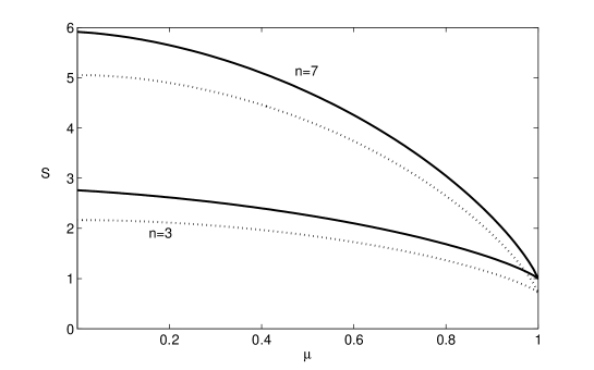
Figure 2: The output entropy of separable(…) and GHZ(—) input states with size $n=3$ and $n=7$, as a function of memory parameter $\mu$ in p=0.4. It seems that entangled states do not have any advantage over separable states for strings of odd length.

To find the eigenvalues of ${\mathcal{E}}(|GHZ\rangle)$ we note that this state is as embedding of blocks of the form:

$$\frac{1}{2}\left(\begin{array}[]{cc}\tilde{P}_{\alpha}+\tilde{P}_{\overline{\alpha}}&\tilde{Q}_{\alpha}+\tilde{Q}_{\overline{\alpha}}\\ \tilde{Q}_{\alpha}+\tilde{Q}_{\overline{\alpha}}&\tilde{P}_{\alpha}+\tilde{P}_{\overline{\alpha}}\end{array}\right),$$ (22)

in different non-overlapping positions of a matrix. Thus the eigenvalues of the output state $\mathcal{E}(|GHZ\rangle)$, are a collection of the eigenvalues of these block. Thus we find the final form of eigenvalues for both input states:

$$\lambda_{\alpha} = \tilde{P}_{\alpha}\hskip 56.9055pt\hskip 56.9055pt\hskip 56.9055ptfor\ \ \ \ |\mathbf{0}\rangle,$$ (23)

$$\lambda_{\alpha} = \frac{1}{2}(\tilde{P}_{\alpha}+\tilde{P}_{\overline{\alpha}}\pm(\tilde{Q}_{\alpha}+\tilde{Q}_{\overline{\alpha}}))\hskip 56.9055pt\ \ for\ \ \ \ |GHZ\rangle.$$ (24)

The subscript, $\alpha=\alpha_{1}\alpha_{2}\cdots\alpha_{N}$, range over the the numbers $\{0,\ 2^{n}-1\}$ for separable states. For the GHZ states the same range of subscripts produces the eigenvalues twice, since $\alpha$ and $\overline{\alpha}$ lead to the same eigenvalues. So the calculated entropy for the whole range of $\alpha\in\{0,2^{n}-1\}$ should be halved to obtain the correct final value.
From these eigenvalues we can calculate the output entropies

$$S_{out}=-\sum_{\alpha}\lambda_{\alpha}\log\lambda_{\alpha}$$

as functions of $p$ and $\mu$. For small values of $n$ the entropy can be evaluated in closed form. However as we increase $n$ the number of eigenvalues increases exponentially and a closed expression is not possible. Figures (2) and (3) show the output entropy for the separable and GHZ states for strings of different length as a function of the memory parameter $\mu$. It is seen that for odd length of the string, the separable states are better than the GHZ states for all values of the memory parameters. However for strings of even-length the GHZ states are better once the memory parameter passes a critical value. Figure (4) shows the value of this critical memory as a function of the length of the string for a typical value of the error parameter. It is seen that as the length of the string increases this critical value increases toward unity. Thus for very large strings we conclude that entangled states loose their advantage over separable states altogether.

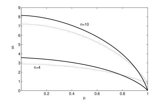
Figure 3: The output entropy of separable (…) and GHZ(—) input states with size $n=4$ and $n=10$, as a function of memory parameter $\mu$ for $p=0.4$. Entangled states seems to have an advantage for strings of even length.

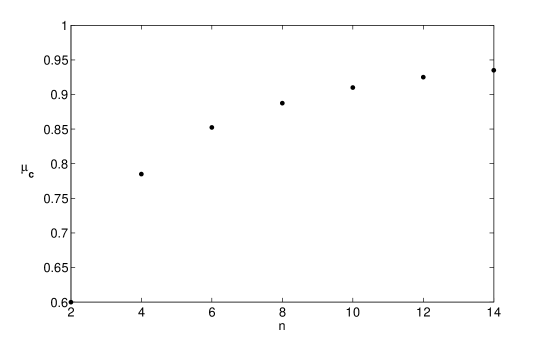
Figure 4: Critical memory as a function of the size of the input string for $p=0.4$.

4 Other types of encoding

In order to substantiate our arguments, we depict in figures (5 ) and (6) the output entropy for several types of other states for strings of length $n=3$ and $n=4$. Each of these states gives rise to an equi-probable ensemble as defined in (13).
The calculations for these types of states have been done as outlined in previous sections. For $n=3$ we have considered the additional states

$$|\psi^{+}\rangle\otimes|0\rangle,\hskip 28.45274pt{\rm and}\hskip 28.45274pt|0\rangle\otimes|\psi^{+}\rangle$$

where $|\psi^{+}\rangle=\frac{1}{\sqrt{2}}(|00\rangle+|11\rangle)$ is a Bell state and a state of the form

$$|W\rangle=\frac{1}{2}(|100\rangle+|010\rangle+|001\rangle+|111\rangle).$$

For $n=4$ we have considered the additional states

$$|\psi^{+}\rangle\otimes|\psi^{+}\rangle,\ \ \ \ \ |\psi^{+}\rangle\otimes|00\rangle,\ \ \ \ |0\rangle\otimes|\psi^{+}\rangle\otimes|0\rangle\ \ \ {\rm and}\ \ \ |00\rangle\otimes|\psi^{+}\rangle.$$

Figure (5) shows that for $n=3$ separable states are optimal for all values of $\mu$ while figures (6) and (7) show that the optimal state changes from a separable state to an entangled state as we increase $\mu$. It is seen that a only a string of two Bell states, or a GHZ state have a lower entropy then the separable state and other forms of partially entangled states are not better than separable states. Moreover it is seen that when the memory parameter increases a string of two Bell states is slightly better than the GHZ state.

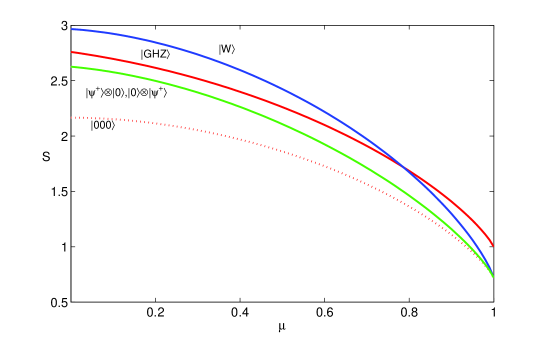
Figure 5: The output entropy for different entangled input strings of length n=3, and $p=0.4$. Separable states are better than other states for strings of odd length.

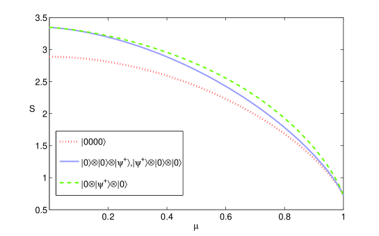
Figure 6: The output entropy for different entangled input strings of length n=4, and $p=0.4$. Again completely separable states have lower entropy than partially entangled strings.

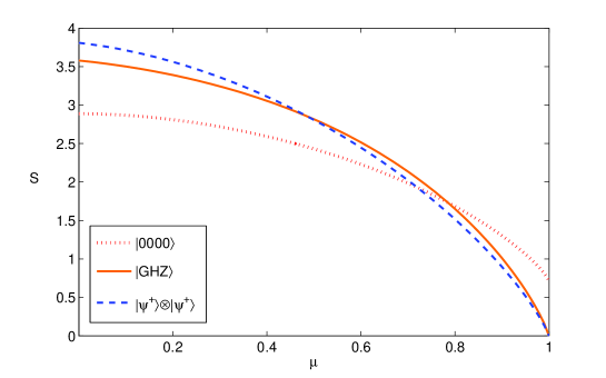
Figure 7: The output entropy for different entangled input strings of length n=4, and $p=0.4$. For high value of memory GHZ and pairs of Bell states take over the separable strings.

5 Summary

We have compared the mutual information for a memory Pauli channel for two ensemble of input states of arbitrary length, a separable ensemble and an ensemble constructed from the entangled GHZ states. Our results show that for odd lengths of the strings, separable states lead to a higher mutual information. However for strings of even length GHZ states outperform the separable states when the memory of the channel exceeds a critical value. The value of this critical memory increases toward unity as the length of the string increases implying that for arbitrarily long sequences still the separable and GHZ states perform equally well.
Although previous works [4, 5, 7, 8, 9] have shown that entangled states are advantageous for encoding classical data into two qubits, our results imply that this advantage may not lead to a higher rate of information transfer, since general theorems of information theory require that only typical sequences be encoded and these should be encoded into arbitrary large sequences for which we have shown that this advantage no longer exists.

6 Appendix A

Here we briefly explain how to calculate the output states of the channel. The derivation is simplified if we relabel the Pauli error operators and the corresponding probabilities by two indices instead of one. Thus the Pauli operators, including the identity operator $I$ are denoted by $\sigma_{{}_{\alpha,\beta}}$ where $\alpha,\beta=0,1$. Such an error operator acts with probability $p_{{}_{\alpha,\beta}}$. We have $\sigma_{0,0}=I,\ \ \sigma_{0,1}=\sigma_{z},\ \ \sigma_{1,0}=\sigma_{x},$ and $\sigma_{1,1}=i\sigma_{y}$ whose actions are compactly written as

$$\sigma_{{}_{\alpha,\beta}}=\sum_{k=0}^{1}(-1)^{\beta k}|k+\alpha\rangle\langle k|.\hskip 28.45274pt\alpha,\beta=0,1.$$ (25)

The channel acts on a single qubit as:

$${\mathcal{E}}^{(1)}(\rho)=\sum_{\alpha,\beta=0}^{1}p_{{}_{\alpha,\beta}}\sigma_{{}_{\alpha\beta}}\rho\sigma_{{}_{\alpha\beta}}^{\dagger}.$$ (26)

From (9) and (10), it’s action on a string of $n$ qubits, is given by :

$${\mathcal{E}}^{(n)}(\rho)=\sum_{\mathbf{\alpha},\mathbf{\beta}=0}^{1}P_{{}_{\mathbf{\alpha},\mathbf{\beta}}}\chi_{{}_{\mathbf{\alpha},\mathbf{\beta}}}(\rho),$$ (27)

in which $\mathbf{\alpha}=\alpha_{1}\alpha_{2}\cdots\alpha_{n}$, $\mathbf{\beta}=\beta_{1}\beta_{2}\cdots\beta_{n}$, and

$$\chi_{{}_{\mathbf{\alpha},\mathbf{\beta}}}(\rho)=(\sigma_{{}_{\alpha_{1}\beta_{1}}}\otimes\sigma_{{}_{\alpha_{2}\beta_{2}}}\cdots\otimes\sigma_{{}_{\alpha_{n}\beta_{n}}})\rho(\sigma_{{}_{\alpha_{1}\beta_{1}}}\otimes\sigma_{{}_{\alpha_{2}\beta_{2}}}\cdots\otimes\sigma_{{}_{\alpha_{n}\beta_{n}}})^{{\dagger}}.$$ (28)

and

$$P_{{}_{\mathbf{\alpha},\mathbf{\beta}}}=\prod_{i=1}^{n-1}\left[(1-\mu)p_{{}_{\alpha_{i}\beta_{i}}}+\mu\delta_{{}_{\alpha_{i}\alpha_{i+1}}}\delta_{{}_{\beta_{i}\beta_{i+1}}}\right]p_{{}_{\alpha_{n}\beta_{n}}}.$$ (29)

It is now easy to calculate the output states of separable and GHZ input states:

$${\mathcal{E}}^{(n)}(|\mathbf{0}\rangle\langle\mathbf{0}|)=\sum_{\mathbf{\alpha},\mathbf{\beta}=0}^{1}P_{{}_{\mathbf{\alpha},\mathbf{\beta}}}\chi_{{}_{\mathbf{\alpha},\mathbf{\beta}}}(|\mathbf{0}\rangle\langle\mathbf{0}|)$$ (30)

and

$${\mathcal{E}}^{(n)}(|GHZ\rangle)=\frac{1}{2}\sum_{\mathbf{\alpha},\mathbf{\beta}=0}^{1}P_{{}_{\mathbf{\alpha},\mathbf{\beta}}}\left[\chi_{{}_{\mathbf{\alpha},\mathbf{\beta}}}(|\mathbf{0}\rangle\langle\mathbf{0}|)+\chi_{{}_{\mathbf{\alpha},\mathbf{\beta}}}(|\mathbf{0}\rangle\langle\mathbf{1}|)+\chi_{{}_{\mathbf{\alpha},\mathbf{\beta}}}(|\mathbf{1}\rangle\langle\mathbf{0}|)+\chi_{{}_{\mathbf{\alpha},\mathbf{\beta}}}(|\mathbf{1}\rangle\langle\mathbf{1}|)\right].$$ (31)

From (28) and (25) we have:

$$\chi_{\mathbf{\alpha},\mathbf{\beta}}(|\mathbf{0}\rangle\langle\mathbf{0}|) = |\mathbf{\alpha}\rangle\langle\mathbf{\alpha}|$$ (32)

$$\chi_{\mathbf{\alpha},\mathbf{\beta}}(|\mathbf{1}\rangle\langle\mathbf{1}|) = |\overline{\mathbf{\alpha}}\rangle\langle\overline{\mathbf{\alpha}}|$$ (33)

$$\chi_{\mathbf{\alpha},\mathbf{\beta}}(|\mathbf{0}\rangle\langle\mathbf{1}|) = |\mathbf{\alpha}\rangle\langle\overline{\mathbf{\alpha}}|(-1)^{\sum_{i=1}^{n}\beta_{i}}$$ (34)

$$\chi_{\mathbf{\alpha},\mathbf{\beta}}(|\mathbf{1}\rangle\langle\mathbf{0}|) = |\overline{\mathbf{\alpha}}\rangle\langle\mathbf{\alpha}|(-1)^{\sum_{i=1}^{n}\beta_{i}},$$ (35)

in which $\overline{\alpha}=\alpha+1$ mod 2. Combining these with (30) the output states are found to be:

$${\mathcal{E}}^{(n)}(|\mathbf{0}\rangle\langle\mathbf{0}|) = \sum_{\mathbf{\alpha},\mathbf{\beta}=0}^{1}P_{\mathbf{\alpha},\mathbf{\beta}}|\mathbf{\alpha}\rangle\langle\mathbf{\alpha}|,$$ (36)

$${\mathcal{E}}^{(n)}(|GHZ\rangle) = \frac{1}{2}\sum_{\mathbf{\alpha},\mathbf{\beta}=0}^{1}P_{\mathbf{\alpha},\mathbf{\beta}}(|\mathbf{\alpha}\rangle\langle\mathbf{\alpha}|+|\overline{\mathbf{\alpha}}\rangle\langle\overline{\mathbf{\alpha}}|)$$ (37)

$$+ \sum_{\mathbf{\alpha},\mathbf{\beta}=0}^{1}P_{\mathbf{\alpha},\mathbf{\beta}}(-1)^{\sum_{n=1}^{N}\beta_{n}}(|\mathbf{\alpha}\rangle\langle\overline{\mathbf{\alpha}}|+|\overline{\mathbf{\alpha}}\rangle\langle\mathbf{\alpha}|).$$ (38)

If we define $\widetilde{P}_{\mathbf{\alpha}}$, and $\widetilde{Q}_{\mathbf{\alpha}}$ as follows:

$$\widetilde{P}_{\mathbf{\alpha}}=\sum_{\mathbf{\beta}=0}^{2^{n}-1}P_{\mathbf{\alpha},\mathbf{\beta}}\hskip 56.9055pt\widetilde{Q}_{\mathbf{\alpha}}=\sum_{\mathbf{\beta}=0}^{2^{n}-1}P_{\mathbf{\alpha},\mathbf{\beta}}(-1)^{\sum_{i=1}^{n}\beta_{i}},$$ (39)

the output states take the simple form:

$${\mathcal{E}}^{(n)}(|\mathbf{0}\rangle\langle\mathbf{0}|) = \sum_{\mathbf{\alpha}=0}^{2^{n}-1}\widetilde{P}_{\mathbf{\alpha}}|\mathbf{\alpha}\rangle\langle\mathbf{\alpha}|,$$ (40)

$${\mathcal{E}}^{(n)}(|GHZ\rangle) = \frac{1}{2}\sum_{\mathbf{\alpha}=0}^{2^{n}-1}\left[\widetilde{P}_{\mathbf{\alpha}}(|\mathbf{\alpha}\rangle\langle\mathbf{\alpha}|+|\overline{\mathbf{\alpha}}\rangle\langle\overline{\mathbf{\alpha}}|)+\widetilde{Q}_{\mathbf{\alpha}}(|\mathbf{\alpha}\rangle\langle\overline{\mathbf{\alpha}}|+|\overline{\mathbf{\alpha}}\rangle\langle\mathbf{\alpha}|)\right].$$ (41)

For a symmetric Pauli channel in which $p_{00}=p_{01}=p$, $p_{10}=p_{11}=q$ and $p+q=\frac{1}{2}$ the expressions of $\tilde{P}_{\alpha}$ and $\tilde{Q}_{\alpha}$ are simplified to

$$\tilde{P}_{\alpha}=\eta_{{\alpha}_{n}}\prod_{i=1}^{n-1}\left[(1-\mu)\eta_{{\alpha}_{i}}+\mu\delta_{\alpha_{i},\alpha_{i+1}}\right],$$ (42)

and

$$\tilde{Q}_{\alpha}=\left\{\begin{array}[]{l}\mu^{\frac{n}{2}}\eta_{{\alpha}_{n}}\delta_{\alpha_{n-1},\alpha_{n}}\prod_{i=1}^{\frac{n}{2}-1}\delta_{\alpha_{2i-1},\alpha_{2i}}\left[(1-\mu)\eta_{{\alpha}_{2i}}+\mu\delta_{\alpha_{2i},\alpha_{2i+1}}\right],\ \ \ n=even\\ \\ 0\hskip 56.9055pt\hskip 56.9055pt\hskip 56.9055pt\hskip 56.9055pt\hskip 28.45274pt\ \ ,\ \ \ \ n=odd\\ \end{array}\right.$$ (43)

where $\eta_{0}=2p$ and $\eta_{1}=2q$.

References

- [1] C. King and M.B. Ruskai, IEEE Trans. Inf. Theory 47,192(2001).
- [2] C. King, quant-ph/0103156
- [3] D. Bruß, L. Faoro, C. Macchiavello, and G.M. Palma, J. Mod. Opt. 47, 325, 2000.
- [4] C. Macchiavello, and G.M. Palma, Phys. Rev. A 65, 050301(R)(2002).
- [5] C. Macchiavello, G.M. Palma, S. Virmani, Phys. Rev. A 69, 010303, (2004).
- [6] M. A. Nielsen, and I. L. Chuang;Quantum computation and quantum information,Cambridge University Press, Cambridge, 2000.
- [7] ,V. Karimipour, L. Memarzadeh, Transition behavior in the capacity of correlated-noisy channels in arbitrary dimensions, quant-ph/0603223, Phys. Rev. A, in press.
- [8] E. Karpov, D. Daems, N. J. Cerf, quant-ph/0603286
- [9] N.J. Cerf, J. Clavareau, C. Macchiavello. and J. Roland, Phys. Rev. A 72, 042330 (2005).
- [10] C. E. Shannon; A mathematical theory of communication, Bell System Tech.J. 27, 379-423, 623-656(1948); C. E. Shannon, W. Weavwe, The mathematical theory of communication, University of Illinois, Urbana(1949)
- [11] B. Schumacher and M. D. Westmoreland, Phys.Rev. A 56, 131-138 (1997).
- [12] W. Dür, G. Vidal, J. I. Cirac, Phys. Rev. A 62, 062314 (2000)