Continuous-Time Quantum Random Walks Require Discrete Space

Abstract

Quantum random walks are shown to have non-intuitive dynamics which makes them an attractive area of study for devising quantum algorithms for long-standing open problems as well as those arising in the field of quantum computing. In the case of continuous-time quantum random walks, such peculiar dynamics can arise from simple evolution operators closely resembling the quantum free-wave propagator. We investigate the divergence of quantum walk dynamics from the free-wave evolution and show that in order for continuous-time quantum walks to display their characteristic propagation, the state space must be discrete. This behavior rules out many continuous quantum systems as possible candidates for implementing continuous-time quantum random walks.

I Introduction

Quantum random walks represent a generalized version of the well known classical random walk, which can be elegantly described using quantum information processing terminology Aharonov et al. (1993). Despite their apparent connection however, dynamics of quantum random walks are often non-intuitive and deviate significantly from those of their classical counterparts Farhi and Gutmann (1998). Among the differences, the faster mixing and hitting times of quantum random walks are particularly noteworthy, making them an attractive area of study for devising efficient quantum algorithms, including those pertaining to connectivity and graph theory Kempe (2003); Farhi and Gutmann (1998); Childs et al. (2003), as well as quantum search algorithms Shenvi et al. (2003); Childs and Goldstone (2004).

There are two broad classes of quantum random walks, namely the discrete- and continuous-time quantum random walks, which have independently emerged out of the study of unrelated physical problems. Despite their fundamentally different quantum dynamics however, both families of walks share similar and characteristic propagation behavior Kempe (2003); Konno (2005); Patel et al. (2005). Strauch’s recent work Strauch (2006) is the latest in a line of theoretical efforts to establishing a formal connection between the discrete and continuous-time quantum random walks, in a manner similar to their classical counterparts.

In this paper we investigate the discretization of space in continuous-time quantum walks. To the best of our knowledge is the first study examining the relationship between discrete- and continuous- space quantum random walks. In what follows we present, in Sec. II, an introductory overview of continuous-time quantum random walks. Then in Sec. III we provide a concise definition of discrete and continuous state space, and in Sec IV describe the way in which we model the transition of the state space from discrete to continuous. We present our results in Sec. V and show how such a transition can reduce the quantum walk evolution to the typical quantum wave propagation in free space. In conclusion we discuss the implications of our findings for the physical implementation of continuous-time quantum random walks. In particular we argue that existing experimental implementations Du et al. (2003); Côté et al. (2006); Solenov and Fedichkin (2006) implicitly verify our assertion that continuous-time quantum random walks require discrete space.

II Continuous-time Quantum Random Walk Overview

Continuous-time quantum random walks were initially proposed by Farhi and Gutmann Farhi and Gutmann (1998) in 1998, out of a study of computational problems formulated in terms of decision trees. Suppose we are given a decision tree that has $N$ nodes indexed by integers $i=1,\ldots,N$. We can then define an $N\times N$ transition rate matrix $\mathcal{H}$ with elements

$$\begin{array}[]{c}h_{ij}=\left\{\begin{array}[]{ll}-\gamma_{ij}&\text{for $i\neq j$ if node $i$ is connected to node $j$}\\ 0&\text{for $i\neq j$ if node $i$ is not connected to node $j$}\\ S_{i}&\text{for $i=j$}\end{array}\right.\end{array},$$ (1)

where $\gamma_{ij}$ is the probability per unit time for making a transition from node $i$ to node $j$ and for $\mathcal{H}$ to be conservative

$$S_{i}=\sum_{\begin{subarray}{c}j=1\\ j\neq i\end{subarray}}^{N}\gamma_{ij}.$$ (2)

Defining $\mathbf{P}$ as the probability distribution vector for the nodes, the transitions can be described by

$$\frac{d\mathbf{P}(t)}{dt}=-\mathcal{H}\mathbf{P}(t),$$ (3)

for which the solution is

$$\mathbf{P}(t)=\exp(-\mathcal{H}t)\mathbf{P}(0),$$ (4)

known as the master equation.

Farhi and Gutmann’s contribution was to propose using the classically constructed transition rate matrix $\mathcal{H}$ to evolve the continuous-time state transitions quantum mechanically. This involved replacing the real valued probability distribution vector $\mathbf{P}(t)$ with a complex valued wave vector $\psi(t)$ and adding the complex notation $\mathbbmtt{i}$ to the evolution exponent, i.e.

$$\psi(t)=\exp(-\mathbbmtt{i}\mathcal{H}t)\psi(0).$$ (5)

Hence the probability distribution vector $\mathbf{P}(t)=\left|\psi(t)\right|^{2}$ and the elements of $\psi(t)$ are the complex amplitudes $\psi(i,t)=\left<i|\psi(t)\right>$ where $|\psi(t)\rangle$ is the state of the entire decision tree system at time $t$. In this quantum evolution the transition matrix $\mathcal{H}$ is required to be Hermitian. This formulation is not limited to discission trees and can be readily applied to the continuous-time quantum random walk on any general undirected graph with $N$ vertices.

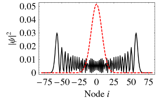
Figure 1: Continuous-time quantum random walk probability distribution (solid) using the transition rate matrix in Eq. 6, with initial condition $\psi(i=0,t=0)=1$ and evolution time $t=15$. Also plotted (dashed) is the time evolution of a continuous-time classical random walk using the same transition rate matrix, initial condition $\mathbf{P}(i=0,t=0)=1$ and evolution time $t=25$.

Figure 1 shows the characteristic probability distribution $\left|\psi(t=15)\right|^{2}$ of a continuous-time quantum random walks on a line with $N=160$ nodes, indexed by $i=-79\ldots 80$, and the initial state $\psi(i=0,t=0)=1$. For this quantum walk each node is assumed to be connected only to its neighboring nodes by a constant transition rate $\gamma=1$ resulting in a transition rate matrix given by

$$\mathcal{H}=\left(\begin{array}[]{ccccc}-2&1&0&0&\\ 1&-2&1&0&\\ 0&1&-2&1&\cdots\\ 0&0&1&-2&\\ &&\vdots&&\ddots\end{array}\right).$$ (6)

For comparison we have also plotted the continuous-time classical random walk probability distribution $\mathbf{P}(t=15)$ using the same transition rate matrix and initial condition $\mathbf{P}(i=0,t=0)=1$.

III Discrete vs Continuous State Space

In Farhi and Gutmann’s treatment of the quantum walk, an arbitrary graph with $N$ vertices can be represented as $N$ position states with coordinate vectors $|\vec{x}_{i}\rangle$, for $i=1,2\ldots N$. These state vectors form an orthonormal basis in the $N$-dimensional Hilbert space $\mathcal{S}$, that is $\left<\vec{x}_{i}|\vec{x}_{j}\right>=\delta_{ij}$ and the wavefunction remains normalized. The time evolution of the quantum walk can be considered as continuously displacing the walker (in time) by a distance $\ell_{ij}$ from node $i$ to all its neighboring nodes $j$ at the rate $\gamma_{ij}$, where $\ell_{ij}=\left\|\vec{x}_{i}-\vec{x}_{j}\right\|$ is defined as the transition length. Since the quantum walker can only be present at positions $\vec{x}_{1},\vec{x}_{2}\ldots\vec{x}_{N}$, we say that the state space is discrete and the walker has an infinitely narrow width. In other words there is no uncertainty or distribution associated with the amplitude

$$\psi(i,t)=\left<\vec{x}_{i}|\psi(t)\right>.$$ (7)

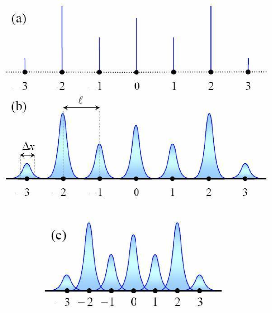
Figure 2: a) Continuous-time quantum random walk on a line of discrete nodes. Vertical lines represent the walker’s probability amplitude to be at each node. d) Continuous-time quantum random walk on a continuous line. The nodes of the walk are a distance $\ell$ apart and localized distributions represent the walker’s probability amplitude to be at each node with an associated uncertainty $\Delta x$. The condition $\ell\gg\Delta x$ means that the nodes are well separated and their respective distributions do not interfere. c) The nodes of the walk have been moved closer such that $\ell\sim\Delta x$. Consequently the localized distributions at neighboring nodes begin to overlap and interfere with one another.

A simple example of this is the quantum walk on a line, illustrated in Fig. 2a, where the position states are discrete nodes arranged in a line and the amplitudes $\psi(i,t)$ are diagrammatically represented as narrow lines over each node. Clearly in this discrete model the nodes can be made arbitrarily close by making $\ell\longrightarrow 0$ without affecting the outcome in any way.

The situation changes however when the state space is continuous, meaning that vector $\vec{x}$ is no longer restricted to coordinates $\vec{x}_{1},\vec{x}_{2}\ldots\vec{x}_{N}$ and the Hilbert space is an infinite dimensional continuum $\mathcal{S}^{\prime}$. A consequence of this is that the quantum walker’s position at $\vec{x}_{i}$ can now have a finite uncertainty associated with it. This is conveniently represented as a distribution with a finite width $\Delta x_{i}$ that is centered at $\vec{x}_{i}$. Taking our previous example of a quantum walk on a line, this continuous model is depicted in Fig. 2b where the amplitude $\psi(i,t)$ is given by the area under the Gaussian distribution centered at $\vec{x}_{i}$.

Despite the continuous nature of the state vectors in $\mathcal{S}^{\prime}$, we can nevertheless use this system to simulate the quantum walk in the discrete Hilbert space $\mathcal{S}$. To implement this virtually-discrete state space over a continuous one, we simply ensure that the states $|\vec{x}_{1}\rangle,|\vec{x}_{2}\rangle\ldots|\vec{x}_{N}\rangle$ remain orthogonal by requiring that the transition length $\ell$ between all the nodes or position states of the walk obeys $\ell\gg\Delta x$. In doing so the overlap between the distributions at the neighboring nodes becomes negligible, which is the case in Fig. 2b.

What we propose here is that the relationship $\ell\gg\Delta x$ is in fact a necessary condition for the quantum random walk to retain its characteristic features. In other words quantum random walks require a discrete or orthonormal state space. In particular we show that for a continuous-time continuous-space quantum walk on a line, where the walker has a finite width, the evolution of the walk is reduced to the conventional quantum wave propagation, in the limit where the transition length approaches a continuum, i.e. $\ell\longrightarrow 0$ (see Fig. 2c).

In what follows we use the finite difference approximation to construct an arbitrary transition rate matrix $\mathcal{H}\approx-\frac{1}{2}\nabla^{2}$ for the quantum walk on a line. We then show that for $\ell\gg\Delta x$ the time evolution results in the characteristic quantum random walk signature as expected. But as the transition length $\ell$ is reduced while keeping $\Delta x$ unchanged, the propagation behavior begins to alter until it converges to that of a quantum wave in free space.

IV Modeling the Discrete to Continuous Transition

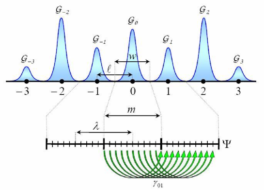
Figure 3: A virtually-discrete quantum walk on a continuous line. The line is divided into segments of length $w$ containing the localized distributions and the transition length between neighboring nodes is $\ell$. This continuous state space is then represented on a numerical vector $\Psi$ with integers $m$ and $\lambda$ corresponding to parameters $w$ and $\ell$ respectively. A transition from node $i$ to node $j$ involves making a transition from all the elements within the $i$th segment to the $j$th segment of the vector.

We start with the continuous state space in Fig. 3 where the continuous position state vector $\vec{x}$ is formally equivalent to a variable $x\in\mathbb{R}$ along a line. This continuous position space is used to construct a virtually-discrete state space quantum walk on a line by ensuring that the condition $\ell\gg\Delta x$ is satisfied. The line is then broken up to adjacent segments of width $w$, with the position of the equidistant nodes $x_{1},x_{2}\ldots x_{N}$ at the center of each segment. The natural uncertainty in the quantum walker’s position at $x_{i}$ is given by a Gaussian distribution

$$\mathcal{G}_{i}(x,t)=\mathcal{A}_{i}(t)\exp\left((x-x_{i})^{2}/(2\Delta x)^{2}\right),$$ (8)

where $\mathcal{A}_{i}(t)$ is a complex phase. The amplitude of the walker to be at position $x_{i}$ is then given by

$$\psi(i,t)=\int_{L_{\min}}^{L_{\max}}\mathcal{G}_{i}(x,t)~{}dx$$ (9)

where $L_{\max}=x_{i}+w/2$ and $L_{\min}=x_{i}-w/2$ are the upper and lower bounds of the block containing the distribution. The condition $w\gg\Delta x$, guarantees that the distribution only finds appreciable values inside this block and is approximately zero elsewhere.

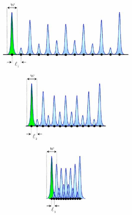
Figure 4: Moving the nodes closer (i.e. $\ell_{1}\rightarrow\ell_{2}\rightarrow\ell_{3}\ldots$) while leaving $w$ unchanged emulates a move from a virtually-discrete to continuous space. This results in the overlap and interferant of the Gaussian distributions at the neighboring nodes.

In the way we have defined the adjacent segments, the width $w$ is equivalent to the transition length $\ell$. What we want to model now is the effect of reducing $\ell$ without changing $w$, which causes the neighboring distributions to overlap as the nodes come closer (see Fig. 4). Keeping $w$ constant is justified as the distribution within the segments is associated with some fundamental uncertainty in the position state which is unaffected by the change in the transition length. The overlap region obviously grows as the nodes get closer while the state space itself (i.e. the line) shrinks as a result. As $\ell\longrightarrow 0$ and the virtually-discrete state space approaches a continuum, it is no longer orthogonal due to the overlapping segments, i.e. $\left|\left<x_{i}|x_{j}\right>\right|>0$ and consequently amplitudes $\psi(i,t)$ as given by Eq. 9 involve summations over some mutual areas.

In order to numerically evolve the quantum walk, we represent the continuous state space of the walk on a finite dimensional complex vector $\Psi$ of length $N\times\lambda$, where $\lambda$ is the integer equivalent of $\ell$, representing the number of elements between $\kappa_{i}$ and $\kappa_{i+1}$, and $\kappa_{1},\kappa_{2}\ldots\kappa_{N}$ are elements of the vector corresponding to the node positions $x_{1},x_{2}\ldots x_{N}$ along the continuous line. We also introduce $m$ as the integer equivalent of $w$, denoting the number of vector elements across each segment.

Given an arbitrary $N\times N$ transition rate matrix $\mathcal{H}$, in order to propagate the quantum walk in the quasi-continuous space represented by vector $\Psi(t)$, we introduce a modified matrix $\mathbf{H}$ of size $N\lambda\times N\lambda$. To construct this matrix, we note that a transition from the $i$th to the $j$th node in the discrete walk corresponds to the transition of all the elements within segment $i$ to segment $j$ as depicted in Fig. 3 and 5. This can be represented by a block matrix

$$\Gamma_{ij}=\left(\begin{array}[]{ccc}0&0&0\\ 0&\mathbf{B}_{ij}&0\\ 0&0&0\\ \end{array}\right)_{N\lambda\times N\lambda},$$ (10)

which is zero everywhere except in an $m\times m$ block

$$\mathbf{B}_{ij}=\gamma_{ij}~{}\mathcal{I}_{m\times m},$$ (11)

which is centered at $\kappa_{i}$ and $\kappa_{j}$, and $\mathcal{I}$ represents the identity matrix. The modified transition matrix is then given by

$$\mathbf{H}=\sum_{i=1}^{N}\sum_{j=1}^{N}\Gamma_{ij},$$ (12)

and the continuous-time quantum random walk proceeds according to

$$\Psi(t)=\exp(-\mathbbmtt{i}\hat{\mathbf{H}}t)\Psi(0).$$ (13)

V Results

In our simulations we considered two quantum walks, both with $N=160$ discrete nodes (enumerated as -79, … 0, … 80) arranged on a line, and transition matrices $\mathcal{H}_{1}$ and $\mathcal{H}_{2}$ which were constructed as the finite difference approximations to $-\frac{1}{2}\nabla^{2}$. For $\mathcal{H}_{1}$ we use the 1${}^{\text{st}}$ order approximation, where

$$\nabla^{2}\psi(i)\approx\frac{1}{2h^{2}}(\psi(i-1)-2\psi(i)+\psi(i+1)).$$ (14)

Here we set grid spacing $h=1$, and the time parameter in $\psi$ is implicit. Transition rates $\gamma_{ij}$ are the coefficients of $\psi(i-s)$ divided by -2, where $i-j=s$ and zero otherwise. $\mathcal{H}_{2}$ is constructed similarly but using the 10${}^{\text{th}}$ order approximation, where

$$\nabla^{2}\psi(i)\approx\frac{1}{25200h^{2}} (8\psi(i-5)-125\psi(i-4)+$$

$$~{}1000\psi(i-3)-6000\psi(i-2)+$$

$$~{}42000\psi(i-1)-73766\psi(i)+42000\psi(i+1)+$$

$$~{}1000\psi(i+3)-6000\psi(i+2)+$$

$$~{}8\psi(i+5)-125\psi(i+4)).$$

For each walk we then defined the vector $\Psi$ using $m=16$ which we initialized so that $\Psi(t=0)$ is zero everywhere except for a single distribution $\mathcal{G}_{i=0}(x,t=0)$ (Eq. 8), corresponding to $\psi(i=0,t=0)=1$. The state space transition from discrete to continuous was then simulated by computing the quantum walk evolution for 5 different values of $\lambda=16,4,3,2$ and 1.

In simulating the walk it is possible to construct the modified transition matrices $\mathbf{H}_{1}$ and $\mathbf{H}_{2}$ as described in the previous section and compute the time evolution from Eq. 13. The evaluation of matrix exponentials however is computationally expensive and even for modest choices of $N$ and $m$, large matrices have to be stored, and the evaluation time becomes prohibitively long, rendering this direct method impractical. Instead in the Appendix we have introduce an alternative computational scheme based on Fourier analysis, which provided us with a dramatic improvement in the computation time.

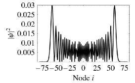
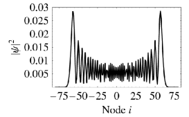
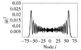
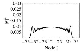
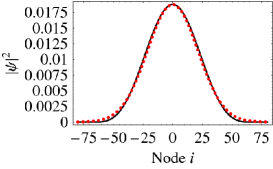
Figure 6: Convergence of the continuous-time quantum random walk probability distribution to a simple Gaussian for transition lengths $\lambda=16,4,3,2,$ and $1$. The evolution is carried out using the coefficients of Eq. 14 as the transition rates, with the initial condition $\psi(i=0,t=0)=1$ and evolution time $t=15$.

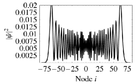
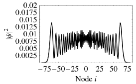
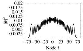
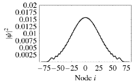
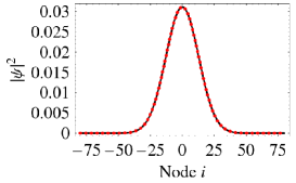
Figure 7: Convergence of the continuous-time quantum random walk probability distribution to a simple Gaussian for transition lengths $\lambda=16,4,3,2,$ and $1$. The evolution is carried out using the coefficients of Eq. V as the transition rates, with the initial condition $\psi(i=0,t=0)=1$ and evolution time $t=15$.

Figures 6 and 7 show the final probability distributions for $\psi(t=15)$ which is obtained using Eq. 9. For the case $\lambda=1$ we have also plotted the analytical solution for the free propagation of a Gaussian wave packet Townsend (1992)

$$\psi_{\mathrm{Gaussian}}(x,t)=\frac{1}{\sqrt{\sqrt{2\pi}(\Delta x+\mathbbmtt{i}t/\Delta x)}}\exp\left(\frac{-x^{2}}{4(\Delta x^{2}+\mathbbmtt{i}t)}\right).$$ (16)

Here we can see an almost perfect convergence of the quantum walk to the familiar propagation of the Gaussian wave packet in free space.

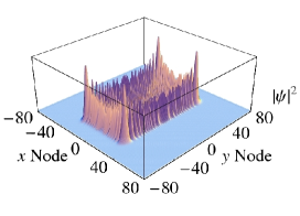
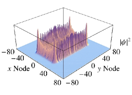
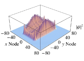
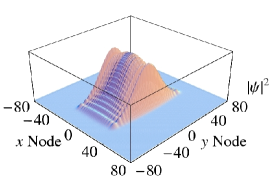
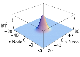
Figure 8: Convergence of a two-dimensional continuous-time quantum random walk probability distribution to a simple Gaussian for transition lengths $\lambda=16,4,3,2,$ and $1$. The evolution is carried out using the coefficients of Eq. 14 and V as transition rates in the $x$ and $y$ directions respectively, with the initial condition $\psi_{\text{2D}}(i=0,j=0,t=0)=1$ and evolution time $t=15$.

Utilizing the computational scheme outlined in the Appendix, extending the above analysis to higher dimensions becomes trivial and computationally viable. Below is an example where we have made the transition from discrete to continuous for a quantum walk on a two-dimensional mesh. The transitions follow $\mathcal{H}_{1}$ in the $x$-direction and $\mathcal{H}_{2}$ in the $y$-direction. The resulting probability distribution for $\psi_{\text{2D}}(t=15)$ is given in Figure 8 where the quantum walk converges from its characteristic evolution to a symmetric Gaussian distribution.

VI Conclusion

We have shown that the evolutionary behavior of continuous-time quantum random walks can be critically affected by the discretization of state space. When the quantum walker has a finite width, a virtually-discrete state space is constructed by keeping the position states of the walk well separated so that their corresponding distributions do not interfere. By allowing the position states to move closer, approaching a continuum, the walker’s distribution at neighboring position states begin to interfere which alters the evolutionary behavior. We have moreover shown that when $\mathcal{H}\approx-\frac{1}{2}\nabla^{2}$ this can even lead to the complete collapse of the quantum walk behavior to that of a typical quantum wave propagation in free space.

Beyond theoretical interest however, our analysis find important implications for the physical implementation of continuous-time quantum random walks. Indeed a number of the existing experimental schemes implicitly verify the notion that state space should be discrete. Du et. al Du et al. (2003) demonstrated the implementation of a quantum walk on a circle with four nodes, using a two-qubit NMR quantum computer. Here the four dimensional state space spanned by the spin states of the two qubits $|\uparrow\uparrow\rangle,|\uparrow\downarrow\rangle,|\downarrow\uparrow\rangle$ and $|\downarrow\downarrow\rangle$, is clearly discrete in nature and the walker has an infinitely narrow width.

Nevertheless the assumption that the walker has a finite width is in fact a realistic one for many other physical systems such as a single particle in real or momentum space, where a localized distribution invariably arises from the fundamental uncertainty in the particle’s position for any given coordinates. In one such proposal Côté et al Côté et al. (2006) described a scheme based on ultra cold Rydberg (highly excited) ⁸⁷Rb atoms in an optical lattice. In this scheme the walk is taking place in real space which is clearly continuous, but the confinement of atomic wavefunction to individual lattice sites amounts to a virtually-discrete state space. In fact Côté et al prescribe an even more conservative condition: to eliminate the atoms except in every fifth site (spacing 25$\mu$m) in order to achieve a better fractional definition of the atom separation. Similarly Solenov and Fedichkin Solenov and Fedichkin (2006) proposed using an a ring shaped array of identical tunnel-coupled quantum dots to implement the continuous-time quantum random walk on a circle. Given the confinement of the electron wavefunction inside the individual quantum dots, the authors have once again implicitly described a virtually-discrete state space over the continuous real space.

APPENDIX: Computational Scheme

Here we present a computationally efficient scheme, referred to as the Fourier-shift method, which not only dramatically speeds up the evaluation of matrix exponential in Eq. 13, but can also be readily extended to higher dimensions when the connections between the nodes naturally form a multidimensional mesh.

Our scheme is applicable to continuous-time quantum walks on $2d$ regular graphs. Specifically for a graph with $N$ vertices or nodes, if we arrange all the nodes in a line indexed as $1,2,\ldots,N$, we require that each node $i$ is connected to nodes $j=i-d,i-d+1,\ldots,i+d-1,i+d$ with transition rates $\gamma_{s}$, where $s=i-j$. Applying these transitions to the $i$th node we have

$$\mathcal{H}\psi(i)=\sum_{s=-d}^{d}\gamma_{s}~{}\psi(i+s),$$ (A-1)

where we have made the time parameter $t$ implicit. Using the notation

$$\overset{\xrightarrow{~{}s~{}}}{(\psi)}_{i}\equiv\psi(i+s),$$ (A-2)

where $\xrightarrow{~{}s~{}}$ represents shifting the entire vector $\psi$ ($s$ nodes in the positive direction if $s>0$, $s$ nodes in the negative direction if $s<0$, and no shift for $s=0$), we can rewrite Eq. A-1 as

$$\mathcal{H}\psi(i)=\sum_{s=-d}^{d}\gamma_{s}~{}\overset{\xrightarrow{~{}s~{}}}{(\psi)}_{i}=\left(\sum_{s=-d}^{d}\gamma_{s}~{}\overset{\xrightarrow{~{}s~{}}}{\psi}\right)_{i},$$ (A-3)

which yields

$$\mathcal{H}\psi=\sum_{s=-d}^{d}\gamma_{s}~{}\overset{\xrightarrow{~{}s~{}}}{\psi}.$$ (A-4)

This representation is desirable since vector shifts can be readily expressed via the Fourier shift theorem, which in turn greatly simplifies the evaluation of $\exp(-\mathbbmtt{i}\mathcal{H}t)$. The discrete Fourier shift theorem states that

$$\mathcal{F}_{k}\left\{\overset{\xrightarrow{~{}s~{}}}{\psi}\right\}=\mathcal{F}_{k}\left\{\psi\right\}p_{k}(s),$$ (A-5)

where $\mathcal{F}_{k}$ represents the $k^{\mathrm{th}}$ element of the discrete Fourier vector with $k=0,1,2\ldots N-1$, and

$$p_{k}(s)=\exp(2\pi\mathbbmtt{i}\widetilde{k}s/N),$$ (A-6)

where $\widetilde{k}=k$ for $k\in[0,N/2]$, and $\widetilde{k}=k-N$ for $k\in[N/2+1,N-1]$. Then applying the inverse transform we have

$$\overset{\xrightarrow{~{}s~{}}}{\psi}=\mathcal{F}^{-1}\left\{\mathcal{F}\left\{\psi\right\}\otimes\mathcal{P}(s)\right\},$$ (A-7)

where $\mathcal{P}(s)$ is a vector with elements $p_{k}(s)$ and $\otimes$ is the direct vector product such that $(a_{1},a_{2},\ldots,a_{n})\otimes(b_{1},b_{2},\ldots,b_{n})=(a_{1}b_{1},a_{2}b_{2},\ldots,a_{n}b_{n})$.

We can now use the above identity to rewrite Eq. A-4 as

$$\mathcal{H}\psi=\mathcal{F}^{-1}\left\{\mathcal{F}\left\{\psi\right\}\otimes\mathcal{Q}\right\},$$ (A-8)

where

$$\mathcal{Q}=\sum_{s=-d}^{d}\gamma_{s}~{}\mathcal{P}(s).$$ (A-9)

This results in the following simplification

$$\mathcal{H}^{n}~{}\psi =\mathcal{F}^{-1}\left\{\ldots\mathcal{F}\left\{\mathcal{F}^{-1}\left\{\mathcal{F}\left\{\psi\right\}\otimes\mathcal{Q}\right\}\right\}\otimes\mathcal{Q}\ldots\right\}$$ (A-10)

$$=\mathcal{F}^{-1}\left\{\mathcal{F}\left\{\psi\right\}\otimes\mathcal{Q}^{n}\right\},$$ (A-11)

where $\mathcal{Q}^{n}$ denotes the direct product of $n$ $\mathcal{Q}$-vectors. Hence a polynomial expansion of Eq. 5 gives

$$\psi(t) =\sum_{n=0}^{\infty}C_{n}(-\mathbbmtt{i}\mathcal{H}t)^{n}\psi(0)$$ (A-12)

$$=\mathcal{F}^{-1}\left\{\mathcal{F}\left\{\psi(0)\right\}\otimes\sum_{n=0}^{\infty}C_{n}(-\mathbbmtt{i}\mathcal{Q}t)^{n}\right\}$$ (A-13)

$$=\mathcal{F}^{-1}\left\{\mathcal{F}\left\{\psi(0)\right\}\otimes\mathcal{R}(t)\right\},$$ (A-14)

where $C_{n}$ are the expansion coefficients and elements $r_{i}(t)$ of vector $\mathcal{R}(t)$ are related to elements $q_{i}$ of vector $\mathcal{Q}$ via the relation $r_{i}(t)=\exp(-\mathbbmtt{i}q_{i}t)$.

Computationally this representation is much more efficient than a direct evaluation of the $N\times N$ matrix exponential in Eq. 5, since vector $\mathcal{Q}$ needs to be calculated once, and for different values of time $t$ we only require the evaluation of $N$ scaler exponentials $\exp(-\mathbbmtt{i}q_{i}t)$ followed by the action of $\mathcal{F}^{-1}\mathcal{F}$ which can be efficiently performed using FFT.

A numerical comparison between the direct and the Fourier-shift method shows an excellent agreement in the resulting probability distributions, while highlighting the Fourier method’s tremendous efficiency. Setting $N=200$ and using the transition rates given by Eq. 14, we were able to compute $\exp(-\mathbbmtt{i}\mathcal{H}_{1}t)$ for $t=5$ and evolve $\psi$ (initialized as a Gaussian distribution with $\Delta x=2$) with a relative accuracy better than $10^{-16}$. Repeating this for $N$ ranging between 50 and 250, we also obtained an efficiency factor $t_{d}/t_{F}$ as a function of $N$, where $t_{d}$ and $t_{F}$ are the CPU times required for the direct and Fourier-shift methods, respectively. This is plotted in Fig 9 along with a quadratic fit to the data. The relatively large deviation of the data from the mean is mainly due to the better optimization of FFT packages for arrays of certain sizes, which should be considered in the actual numerical implementation.

We can now extend Eq. A-14 for application to the quasi-continuous quantum walk on vector $\Psi$ where each node is represented by a segment of $m$ elements in the vector. In this case transition from node $i$ to node $j$ is equivalent to the vector elements within the $i$th segment making a transition of length $\lambda\left|i-j\right|$. It is then easy to defining $(N\times\lambda)$-element equivalents for vectors $\mathcal{P}(s)$, $\mathcal{Q}$ and $\mathcal{R}$, represented by $\mathcal{\overline{P}}(s)$, $\mathcal{\overline{Q}}$ and $\mathcal{\overline{R}}$, and adjust the vector shifts by a factor $\lambda$. More explicitly, the elements of $\mathcal{\overline{P}}(s)$ are given by

$$\overline{p}_{k}(s)=\exp(2\pi\mathbbmtt{i}\widetilde{k}s/\overline{N}),$$ (A-15)

where $\overline{N}=N\lambda$, and

$$\mathcal{\overline{Q}}=\sum_{s=-\lambda d}^{\lambda d}\gamma_{s}~{}\mathcal{\overline{P}}(s).$$ (A-16)

$\mathcal{\overline{R}}(t)$ is then constructed as before with elements $\overline{r}_{i}(t)=\exp(-\mathbbmtt{i}\overline{q}_{i}t)$ and the time evolution of the quantum walk over $\Psi$ is simply given by

$$\Psi(t)=\mathcal{F}^{-1}\left\{\mathcal{F}\left\{\Psi(0)\right\}\otimes\mathcal{\overline{R}}(t)\right\}.$$ (A-17)

VII Figures

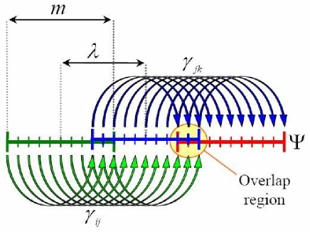
Figure 5: Approaching the nodes of the quantum walk represented on vector $\Psi$ involves reducing $\lambda$ while leaving $m$ unchanged which leads to an overlap region where vector elements are shared by neighboring distributions. A transition from node $i$ to node $j$ involves making a transition from all the elements within the $i$th segment to the $j$th segment of the vector. Vector elements in the overlap region are subject to the cumulative transition of the overlapping nodes.

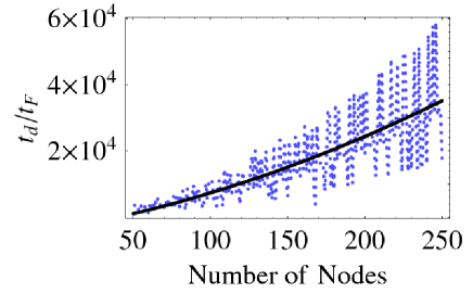
Figure 9: The computational efficiency of the Fourier-shift method over the direct method as a function of the number of nodes. The solid curve represents a quadratic fit to the efficiency data (dotted).

References

- Aharonov et al. (1993) Y. Aharonov, L. Davidovich, and N. Zagury, Phys. Rev. A 48, 1687 (1993).
- Farhi and Gutmann (1998) E. Farhi and S. Gutmann, Phys. Rev. A 58, 915 (1998).
- Kempe (2003) J. Kempe, Contemporary Physics 44, 307 (2003).
- Childs et al. (2003) A. M. Childs, R. Cleve, E. Deotto, E. Farhi, S. Gutmann, and D. A. Spielman, Proc. 35th ACM Symposium on Theory of Computing pp. 59–68 (2003).
- Shenvi et al. (2003) N. Shenvi, J. Kempe, and K. B. Whaley, Phys. Rev. A 67, 052307 (2003).
- Childs and Goldstone (2004) A. M. Childs and J. Goldstone, Phys. Rev. A 70, 022314 (2004).
- Konno (2005) N. Konno, Phys. Rev. E 72, 26113 (2005).
- Patel et al. (2005) A. Patel, K. S. Raghunathan, and P. Rungta, Phys. Rev. A 71, 32347 (2005).
- Strauch (2006) F. W. Strauch, Phys. Rev. A 74, 030301 (2006).
- Du et al. (2003) J. Du, H. Li, X. Xu, M. Shi, J. Wu, X. Zhou, and R. Han, Phys. Rev. A 67, 042316 (2003).
- Côté et al. (2006) R. Côté, A. Russell, E. E. Eyler, and P. L. Gould, New Jour. Phys. 8, 156 (2006).
- Solenov and Fedichkin (2006) D. Solenov and L. Fedichkin, Phys. Rev. A 73, 012313 (2006).
- Townsend (1992) J. S. Townsend, A Modern Approach to Quantum Mechanics (McGraw-Hill, 1992).