Force on a neutral atom near conducting microstructures

Abstract

We derive the non-retarded energy shift of a neutral atom for two different geometries. For an atom close to a cylindrical wire we find an integral representation for the energy shift, give asymptotic expressions, and interpolate numerically. For an atom close to a semi-infinite halfplane we determine the exact Green’s function of the Laplace equation and use it derive the exact energy shift for an arbitrary position of the atom. These results can be used to estimate the energy shift of an atom close to etched microstructures that protrude from substrates.

I Introduction

An important aim of current experimental cold atom physics is to learn how to control and manipulate single or few atom in traps or along guides. To this end more and more current and recent experiments deal with atoms close to microstructures, most importantly wires and chips of various kinds (cf. e.g. Schmiedmayr ; Zimmermann ; Hinds ; Vuletic ). If these microstructures carry strong currents then the resulting magnetic fields and possibly additional external fields often create the dominant forces on the atoms, which can then by used for trapping and manipulation. However, since an atom is essentially a fluctuating dipole, polarization effects in those microstructures lead to forces on the atoms even in the absence of currents and external fields, and for atoms very close to them these can be significant. Provided there is no direct wave-function overlap, i.e. the atom is at least a few Bohr radii away from the microstructure, the only relevant force is then the Casimir-Polder force CasimirPolder , which is the term commonly used for the van der Waals force between a point-like polarizable particle and an extended object, in this case – the atom and the microstructure.

The type of microstructures that can be used for atom chips and can be efficiently manufactured often involve a ledge protruding from an electroplated and subsequently etched substrate private . Here we model this type of system in two ways: first by a cylindrical wire (which is a good model for situations where the reflectivity of the electroplated top layer far exceeds that of the substrate), and second by a semi-infinite halfplane (which is an applicable model if the reflectivities of the top layer and substrate do not differ by much). While in reality the electromagnetic reflectivity of a material is of course never perfect, it has been shown by earlier research that interaction with imperfectly reflecting surfaces leads to a Casimir-Polder force that differs only by a minor numerical factor from the one for a perfectly reflecting surface wylie ; wu . Thus we shall consider only perfectly reflecting surfaces here, which keeps the difficulty of the mathematics involved to a reasonable level.

II Energy shift and Green’s function

We would like to consider an atom close to a reflecting surface and work out the energy shift in the atom due to the presence of the surface. As is well known, if the distance of the atom to the surface is much smaller than the wavelength of a typical internal transition, then the interaction with the surface is dominated by non-retarded electrostatic forces CasimirPolder ; Barton ; wu . At larger distances retardation matters, but at the same time the Casimir-Polder force is then significantly smaller and thus hard to measure experimentally (see e.g. sukenik ; inguscio ; cornell ). In this paper we shall concentrate on small distances that lie within the non-retarded electrostatic regime, as these lie well within the range of the experimentally realizable distances of cold atoms from microstructures private .

In order to determine this electrostatic energy shift one needs to solve the (classical) Poisson equation for the electrostatic potential $\Phi$

$$-\boldsymbol{\nabla}^{2}\Phi=\frac{\rho}{\varepsilon_{0}}$$ (1)

with the boundary condition that $\Phi=0$ on the surface of a perfect reflector. The charge density $\rho$ would be the atomic dipole $\boldsymbol{\mu}$ of charges $\pm q$ separated by a vector ${\bf D}$, i.e.

$$\rho(\mathbf{r})=\lim_{{\bf D}\rightarrow 0}\,q\left[\,\delta^{(3)}(\mathbf{r}-(\mathbf{r}_{0}+{\bf D}))-\delta^{(3)}(\mathbf{r}-\mathbf{r}_{0})\right]$$ (2)

for a dipole located at $\mathbf{r}_{0}$. Since the dipole is made up of two point charges, one can find a solution to the Poisson equation (1) via the Green’s function $G(\mathbf{r},\mathbf{r}^{\prime})$, which satisfies

$$-\boldsymbol{\nabla}^{2}G(\mathbf{r},\mathbf{r}^{\prime})=\delta^{(3)}(\mathbf{r}-\mathbf{r}^{\prime})\;,$$ (3)

subject to the boundary condition that it vanishes for all points $\mathbf{r}$ that lie on the perfectly reflecting surface. For the purposes of this paper it is advantageous to split the Green’s function in the following way,

$$G(\mathbf{r},\mathbf{r}^{\prime})=\frac{1}{4\pi|\mathbf{r}-\mathbf{r}^{\prime}|}+G_{H}(\mathbf{r},\mathbf{r}^{\prime})\;.$$ (4)

The first term is the Green’s function of the Poisson equation in unbounded space, and thus the second term is a solution of the homogeneous Laplace equation, chosen in such a way that the sum satisfies the boundary conditions required of $G(\mathbf{r},\mathbf{r}^{\prime})$.

The total energy of the charge distribution is given by stratton

$$E=\frac{1}{2}\int\mathrm{d}^{3}\mathbf{r}\;\rho(\mathbf{r})\Phi(\mathbf{r})\;,$$ (5)

with

$$\Phi(\mathbf{r})=\frac{1}{\varepsilon_{0}}\int\mathrm{d}^{3}\mathbf{r}^{\prime}\ G(\mathbf{r},\mathbf{r}^{\prime})\,\rho(\mathbf{r}^{\prime})$$ (6)

Thus for a dipole with the charge density (2) the total energy is

$$E= \lim_{{\bf D}\rightarrow 0}\bigg{\{}\frac{1}{8\pi\varepsilon_{0}}\frac{q^{2}}{|\mathbf{r}+{\bf D}-(\mathbf{r}+{\bf D})|}+\frac{1}{8\pi\varepsilon_{0}}\frac{q^{2}}{|\mathbf{r}-\mathbf{r}|}$$ (7)

$$-\frac{1}{8\pi\varepsilon_{0}}\frac{q^{2}}{|\mathbf{r}+{\bf D}-\mathbf{r}|}-\frac{1}{8\pi\varepsilon_{0}}\frac{q^{2}}{|\mathbf{r}-(\mathbf{r}+{\bf D})|}$$

$$+\frac{q^{2}}{2\varepsilon_{0}}\left[G_{H}(\mathbf{r}_{0}+{\bf D},\mathbf{r}_{0}+{\bf D})-G_{H}(\mathbf{r}_{0}+{\bf D},\mathbf{r}_{0})\right]$$

$$-\frac{q^{2}}{2\varepsilon_{0}}\left[G_{H}(\mathbf{r}_{0},\mathbf{r}_{0}+{\bf D})-G_{H}(\mathbf{r}_{0},\mathbf{r}_{0})\right]\bigg{\}}\;.$$

The first two terms in this expression are the divergent self-energies of the two point charges. The third and fourth terms are the energy of the dipole, which also diverges in the limit ${\bf D}\rightarrow 0$. None of these are interesting for us because they are the same no matter where the dipole is located. The energy shift due to the presence of the surface is given by the remaining four terms, which all depend just on the homogeneous solution $G_{H}(\mathbf{r},\mathbf{r}^{\prime})$. In the limit ${\bf D}\rightarrow 0$ these four terms can be written as derivatives of $G_{H}$, and thus we obtain for the energy shift of a dipole $\boldsymbol{\mu}=q{\bf D}$ due to the presence of the surface

$$\Delta E=\left.\frac{1}{2\varepsilon_{0}}(\boldsymbol{\mu}\cdot\boldsymbol{\nabla})(\boldsymbol{\mu}\cdot\boldsymbol{\nabla^{\prime}})\;G_{H}(\mathbf{r},\mathbf{r}^{\prime})\right|_{\mathbf{r}=\mathbf{r}_{0},\mathbf{r}^{\prime}=\mathbf{r}_{0}}\;,$$ (8)

where $\mathbf{r}_{0}$ is the location of the dipole.

When applying this to an atom one also needs to take into account that for an atom without permanent dipole moment the quantum-mechanical expectation value of a product of two components of the dipole moment is diagonal,

$$\langle\mu_{i}\mu_{j}\rangle=\langle\mu_{i}^{2}\rangle\>\delta_{ij}\;,$$ (9)

in any orthogonal coordinate system. This implies that for an atom the energy shift due to the presence of the surface reads

$$\Delta E=\left.\frac{1}{2\varepsilon_{0}}\sum_{i=1}^{3}\langle\mu_{i}^{2}\rangle\nabla_{i}\nabla_{i}^{\prime}\;G_{H}(\mathbf{r},\mathbf{r}^{\prime})\right|_{\mathbf{r}=\mathbf{r}_{0},\mathbf{r}^{\prime}=\mathbf{r}_{0}}\;.$$ (10)

Thus the central task in working out the non-retarded energy shift of an atom in the vicinity of a surface is to work out the electrostatic Green’s function of the boundary-value problem for the geometry of this surface. In the next two sections we are going to do this for two different surfaces: for a cylindrical wire of radius $R$ and for a semi-infinite halfplane. In either case we assume that the surfaces are perfectly reflecting, which enforces the electrostatic potential $\Phi$ to vanish there.

III Non-retarded energy shift near a wire

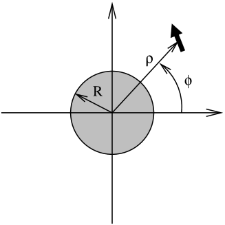
Figure 1: An illustration of the geometry of the dipole near a wire. The radius of the wire is $R$, and the distance of the dipole from the centre of the wire is $\rho$.

To calculate the energy shift, we first determine the Green’s function of the Poisson equation in the presence of a perfectly reflecting cylinder of radius $R$ and infinite length. A standard method of calculating Green’s functions is via the eigenfunctions of the differential operator. In order to find a solution to Eq. (3) we solve the eigenvalue problem

$$-\boldsymbol{\nabla}^{2}\psi_{n}(\mathbf{r})=\lambda_{n}\;\psi_{n}(\mathbf{r})\;.$$ (11)

The eigenfunctions $\psi_{n}(\mathbf{r})$ must satisfy the same boundary conditions as required of the Green’s function. Since $-\boldsymbol{\nabla}^{2}$ is Hermitean, the set of all its normalized eigenfunctions must be complete,

$$\sum_{n}|\psi_{n}(\mathbf{r})\rangle\langle\psi_{n}(\mathbf{r}^{\prime})|=\delta^{(3)}(\mathbf{r}-\mathbf{r}^{\prime})\;.$$ (12)

Thus one can write

$$G(\mathbf{r},\mathbf{r}^{\prime})=\sum_{n}\frac{|\psi_{n}(\mathbf{r})\rangle\langle\psi_{n}(\mathbf{r}^{\prime})|}{\lambda_{n}}\;.$$ (13)

If we apply this method to unbounded space we can easily derive a representation of the Green’s function in unbounded space in cylindrical coordinates,

$$\frac{1}{4\pi|\mathbf{r}-\mathbf{r}^{\prime}|}=\frac{1}{4\pi^{2}}\sum_{m=-\infty}^{\infty}\int_{-\infty}^{\infty}\mathrm{d}\kappa\int_{0}^{\infty}\mathrm{d}k\ \frac{k}{k^{2}+\kappa^{2}}\ \$$

$$\times{\rm e}^{{\rm i}m(\phi-\phi^{\prime})+{\rm i}\kappa(z-z^{\prime})}J_{m}(k\rho)J_{m}(\kappa\rho^{\prime})\;.$$ (14)

Performing the $k$ integration (GR, , 6.541(1.)), we find

$$\frac{1}{4\pi|\mathbf{r}-\mathbf{r}^{\prime}|}= \frac{1}{2\pi^{2}}\sum_{m=-\infty}^{\infty}\int_{0}^{\infty}\mathrm{d}\kappa\ {\rm e}^{{\rm i}m(\phi-\phi^{\prime})+{\rm i}\kappa(z-z^{\prime})}$$ (15)

$$\times I_{m}(\kappa\rho)K_{m}(\kappa\rho^{\prime})\;,\mbox{\ for\ }\rho<\rho^{\prime}\;.$$

To derive the Green’s function (4) that vanishes on the surface of the cylinder $\rho=R$ we now just need to find the appropriate homogeneous solution $G_{H}(\mathbf{r},\mathbf{r}^{\prime})$, which satisfies

$$-\boldsymbol{\nabla}^{2}G_{H}(\mathbf{r},\mathbf{r}^{\prime})=0\;.$$ (16)

The general solution of the homogeneous Laplace equation in cylindrical coordinates can be written as

$$\sum_{m=-\infty}^{\infty}\int_{0}^{\infty}\mathrm{d}\kappa\ {\rm e}^{{\rm i}m\phi+{\rm i}\kappa z}\left[A(m,\kappa)I_{m}(\kappa\rho)+B(m,\kappa)K_{m}(\kappa\rho)\right]$$ (17)

where $A$ and $B$ are some constants. Since $G(\mathbf{r},\mathbf{r}^{\prime})$ and therefore $G_{H}(\mathbf{r},\mathbf{r}^{\prime})$ must be regular at infinite $\rho$ we must have $A(m,\kappa)=0$. This and the requirement that the sum of Eq. (15) and $G_{H}(\mathbf{r},\mathbf{r}^{\prime})$ must vanish at $\rho=R$ lead to

$$G_{H}(\mathbf{r},\mathbf{r}^{\prime})= -\frac{1}{2\pi^{2}}\sum_{m=-\infty}^{\infty}\int_{0}^{\infty}\mathrm{d}\kappa\ {\rm e}^{{\rm i}m(\phi-\phi^{\prime})+{\rm i}\kappa(z-z^{\prime})}$$ (18)

$$\times\frac{I_{m}(\kappa R)}{K_{m}(\kappa R)}\;K_{m}(\kappa\rho)K_{m}(\kappa\rho^{\prime})\;.$$

The energy shift can now be determined by applying formula (10) in cylindrical coordinates. Taking into account the symmetry properties of the modified Bessel functions we find for the energy shift of an atom whose location is given through $(\rho,\phi,z)$

$$\Delta E=-\frac{1}{4\pi\varepsilon_{0}}\left[\Xi_{\rho}\langle\mu_{\rho}^{2}\rangle+\Xi_{\phi}\langle\mu_{\phi}^{2}\rangle+\Xi_{z}\langle\mu_{z}^{2}\rangle\right]$$ (19)

with the abbreviations

$$\Xi_{\rho} \!\!= \!\!\frac{2}{\pi}\sum_{m=0}^{\infty}{}^{\prime}\int_{0}^{\infty}\mathrm{d}\kappa\ \kappa^{2}\frac{I_{m}(\kappa R)}{K_{m}(\kappa R)}\left[K_{m}^{\prime}(\kappa\rho)\right]^{2}$$

$$\Xi_{\phi} \!\!= \!\!\frac{2}{\pi\rho^{2}}\sum_{m=1}^{\infty}\ m^{2}\int_{0}^{\infty}\mathrm{d}\kappa\ \frac{I_{m}(\kappa R)}{K_{m}(\kappa R)}\left[K_{m}(\kappa\rho)\right]^{2}$$

$$\Xi_{z} \!\!= \!\!\frac{2}{\pi}\sum_{m=0}^{\infty}{}^{\prime}\int_{0}^{\infty}\mathrm{d}\kappa\ \kappa^{2}\frac{I_{m}(\kappa R)}{K_{m}(\kappa R)}\left[K_{m}(\kappa\rho)\right]^{2}\;.$$

The prime on the sums indicates that the $m=0$ term is weighted by an additional factor 1/2.

Using numerical integration packages like those built into Mathematica or Maple, one can evaluate these contributions to the energy shift. We show the numerical results in Figs. 2–4. We have chosen to show the various contributions to Eq. (19) as a function of the ratio of the distance $d=\rho-R$ of the atom from the surface of the wire to the wire radius $R$ and multiplied by $d^{3}$ so as to plot dimensionless quantities.

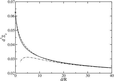
Figure 2: The energy shift due to the $z$ component of the atomic dipole, multiplied by $d^{3}$, where $d$ is the distance of the dipole to the surface of the wire. The solid line is the exact expression calculated numerically, the dot-dashed line is the $m=0$ term alone, and the dashed line is the $m=0$ term plus the single integral derived through the uniform asymptotic approximation for the Bessel functions, Eq. (20c). The cross on the vertical axis gives the exact value for $d\rightarrow 0$.

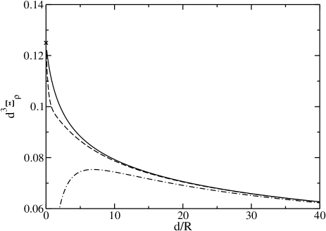
Figure 3: Same as Fig. 2 but for the energy shift due to the $\rho$ component of the atomic dipole. The solid line is the exact expression calculated numerically, the dot-dashed line is the $m=0$ term alone, and the dashed line is the $m=0$ term plus the single integral derived through the uniform asymptotic approximation for the Bessel functions, Eq. (20a).

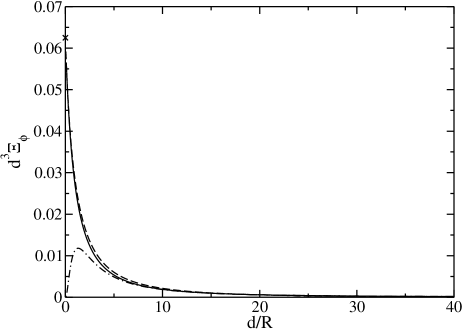
Figure 4: Same as Fig. 2 but for the energy shift due to the $\phi$ component of the atomic dipole.The solid line is the exact expression calculated numerically, the dot-dashed line is the $m=1$ term alone, and the dashed line is the single integral derived through the uniform asymptotic approximation for the Bessel functions, Eq. (20b).

For most values of $d=\rho-R$ the integrals over $\kappa$ converge quite well, as for large $\kappa$ the dominant behaviour of integrands is as $\exp(-2\kappa d)$. Likewise is the convergence of the sums over $m$ very good for reasonably large values of $d$. In fact, as shown by dot-dashed lines in Figs. 2–4, convergence is so good that from $d/R\approx 20$ upwards it is fully sufficient to take just the first summand in each sum for $\Xi$. However, convergence is less good for small $d$ and thus the numerical evaluation of the energy shift gets more and more cumbersome the closer the atom is to the surface of the wire. Neither the integrals over $\kappa$ nor the sums over $m$ converge very well, so that it is worthwhile finding a suitable approximation for small $d$. Another motivation for a detailed analysis of the limit $d\rightarrow 0$ is of course also to check consistency: if the atom is very close to the surface of the wire ($d\ll R$) then the curvature of the wire cannot have any impact on the shift any longer and the energy shift should simply be that of an atom close to a plane surface, which is well known planeshift .

To find a suitable approximation for small $d$, we separate off the $m=0$ terms in $\Xi_{\rho}$ and $\Xi_{z}$. In all the other summands and in $\Xi_{\phi}$ we scale by making a change of variables in the integrals to a new integration variable $x=\kappa\rho/m$. The dominant contributions to those integrals and the sums come from large $x$ and large $m$, so that one can approximate the Bessel functions by their uniform asymptotic expansion (AS, , 9.7.7–10). Then the Bessel functions then the sums over $m$ become geometric series and can be summed analytically. Taking just the leading term in the uniform asymptotic expansions for the Bessel functions we find the following approximations,

$$\Xi_{\rho} \!\!\approx \!\!\frac{1}{\pi}\int_{0}^{\infty}\mathrm{d}\kappa\ \kappa^{2}\frac{I_{0}(\kappa R)}{K_{0}(\kappa R)}\left[K_{1}(\kappa\rho)\right]^{2}$$ (20a)

$$\hskip 19.91692pt+\frac{1}{\pi\rho^{3}}\int_{0}^{\infty}\mathrm{d}x\;\sqrt{1+x^{2}}\;\frac{A(A+1)}{(1-A)^{3}}$$

$$\Xi_{\phi} \!\!\approx \!\!\frac{1}{\pi\rho^{3}}\int_{0}^{\infty}\mathrm{d}x\;\frac{1}{\sqrt{1+x^{2}}}\;\frac{A(A+1)}{(1-A)^{3}}$$ (20b)

$$\Xi_{z} \!\!\approx \!\!\frac{1}{\pi}\int_{0}^{\infty}\mathrm{d}\kappa\ \kappa^{2}\frac{I_{0}(\kappa R)}{K_{0}(\kappa R)}\left[K_{0}(\kappa\rho)\right]^{2}$$ (20c)

$$\hskip 19.91692pt+\frac{1}{\pi\rho^{3}}\int_{0}^{\infty}\mathrm{d}x\;\frac{x^{2}}{\sqrt{1+x^{2}}}\;\frac{A(A+1)}{(1-A)^{3}}$$

with the abbreviation

$$A(x)=\frac{R^{2}}{\rho^{2}}\;{\rm e}^{-2\left(\sqrt{1+x^{2}}-\sqrt{1+x^{2}\frac{R^{2}}{\rho^{2}}}\right)}\left(\frac{1+\sqrt{1+x^{2}}}{1+\sqrt{1+x^{2}\frac{R^{2}}{\rho^{2}}}}\right)^{2}.$$

These are easy to evaluate numerically. We show the numerical values as dashed lines in Figs. 2–4. Furthermore, these approximations allow us to take the limit $d\rightarrow 0$. Taking this limit under the $x$ integrals and retaining only the leading terms in each case, we can carry out the $x$ integrations analytically and obtain

$$\Xi_{\rho}\approx\frac{1}{8d^{3}}\ ,\ \ \Xi_{\phi}\approx\frac{1}{16d^{3}}\ ,\ \ \Xi_{z}\approx\frac{1}{16d^{3}}\;.$$ (21)

Inserting these values into Eq. (19) we see that they give the energy shift of an atom in front a perfectly reflecting plane planeshift . This is an important consistency check for our calculation, as the atom should not feel the curvature of the surface at very close range. In Figs. 2–4 the limiting values (21) are marked as crosses on the vertical axes. Since we have taken along only first term of the uniform asymptotic expansion for each of the Bessel functions, we cannot expect any agreement of the approximations (20a–c) beyond leading order. However, in practice these approximations work quite well beyond leading order: as Figs. 2–4 show, approximations (20b) and (20c) work very well for almost the entire range of $d$; approximation (20a) works reasonably well for small $d$ and then again for large $d$ (because at large distances the $m=0$ term dominates everything else). In this context we should also point out that the $m=0$ contributions to $\Xi_{\rho}$ and $\Xi_{z}$ do not contribute to leading order, but behave as $d^{-2}$ in the limit $d\rightarrow 0$ and thus need to be taken into account for asymptotic analysis in this limit beyond leading order.

At large distances $d$ the energy shift (19) is dominated by the first terms in each of the sums over $m$, i.e. the $m=0$ terms for $\Xi_{\rho}$ and $\Xi_{z}$ and the $m=1$ term for $\Xi_{\phi}$. For large $d$ $\Xi_{\rho}$ and $\Xi_{z}$ behave as $1/(d^{3}\ln d)$, but there is no point in giving an asymptotic expression as further corrections are smaller only by additional powers of $1/\ln d$ and these series converge far too slowly to be of any practical use. $\Xi_{\phi}$ falls off faster: to leading order we get $\Xi_{\phi}\approx 3\pi R^{2}/(32d^{5})$ for large $d$.

Furthermore, if $d$ is not just large compared to $R$ but also compared to the typical wavelength of an internal transition in the atom, then the energy shift would be dominated by retardation effects, which cannot be calculated with the electrostatic approach of this paper, but which require a quantization of the electromagnetic field Barton . For this reason the extreme large-distance limit of the energy shift (19) is not of practical importance and thus we see no reason to report on it in more detail.

IV Non-retarded energy shift near a semi-infinite halfplane

Next we wish to calculate the energy shift of an atom in the vicinity of a perfectly reflecting halfplane. The geometry is sketched in Fig. 5.

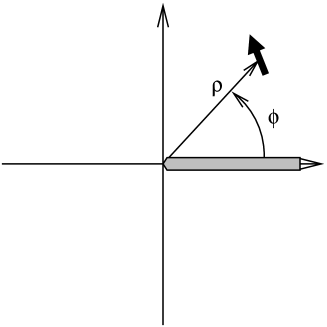
Figure 5: An illustration of the geometry of a dipole near a semi-infinite halfplane. The distance of the dipole from the edge is $\rho$, and from the surface of the plane it is $\rho\sin\phi$.

The required boundary conditions are that the electrostatic potential $\Phi(\mathbf{r})$ vanishes at the angles $\phi=0$ and $\phi=2\pi$. We shall calculate the Green’s function for this case by using the method of summation over eigenfunctions of the operator $-\boldsymbol{\nabla}^{2}$, as explained at the beginning of Section III. If we determine the set of eigenfunctions $\psi_{n}(\mathbf{r})$ that satisfy the correct boundary conditions then the Green’s function (13) will also satisfy these boundary conditions. Normalized eigenfunctions that vanish at $\phi=0$ and $\phi=2\pi$ and that are regular at the origin and at infinity are in cylindrical coordinates

$$\psi_{n}(\rho,\phi,z)=\frac{1}{\sqrt{2\pi}}\,{\rm e}^{{\rm i}\kappa z}\;J_{m/2}(k\rho)\;\frac{1}{\sqrt{\pi}}\sin\frac{m\phi}{2}\;,$$ (22)

with the corresponding eigenvalue $\lambda_{n}=\kappa^{2}+k^{2}$. Construction (13) then gives the Green’s function

$$G(\mathbf{r},\mathbf{r}^{\prime})=\frac{1}{2\pi^{2}}\sum_{m=1}^{\infty}\int_{0}^{\infty}\mathrm{d}k\int_{-\infty}^{\infty}\mathrm{d}\kappa\ \frac{k}{\kappa^{2}+k^{2}}\;{\rm e}^{{\rm i}\kappa(z-z^{\prime})}$$

$$\times\;J_{\frac{m}{2}}(k\rho)J_{\frac{m}{2}}(k\rho^{\prime})\;\sin\frac{m\phi}{2}\sin\frac{m\phi^{\prime}}{2}\;.$$

This result is in agreement with the limiting case of the Green’s function for the electrostatic potential at a perfectly reflecting wedge smythe if the wedge is to be taken to subtend a zero angle and extent to an infinite radius.

As the energy shift (10) depends only on the homogeneous part $G_{H}(\mathbf{r},\mathbf{r}^{\prime})$ of the solution, we need, according to Eq. (4), to subtract the free-space Green’s function, which we have already written down in Eq. (14). Noting that the free-space Green’s function is of course symmetric under the exchange of $\phi$ and $\phi^{\prime}$, we can write it in the form

$$\frac{1}{4\pi|\mathbf{r}-\mathbf{r}^{\prime}|}=\frac{1}{2\pi^{2}}\sum_{m=0}^{\infty}{}^{\prime}\int_{-\infty}^{\infty}\mathrm{d}\kappa\int_{0}^{\infty}\mathrm{d}k\ \frac{k}{k^{2}+\kappa^{2}}\;{\rm e}^{{\rm i}\kappa(z-z^{\prime})}$$

$$\times\cos m(\phi-\phi^{\prime})\;J_{m}(k\rho)J_{m}(\kappa\rho^{\prime})\;.$$

Taking the difference between $G(\mathbf{r},\mathbf{r}^{\prime})$ above and this expression and carrying out the integration over $\kappa$ by closing the contour in the complex plane and determining the residue, we obtain

$$G_{H}(\mathbf{r},\mathbf{r}^{\prime}) \!\!= \!\!-\frac{1}{4\pi}\int_{0}^{\infty}\mathrm{d}k\ {\rm e}^{-k|z-z^{\prime}|}\left\{\sum_{m=0}^{\infty}{}^{\prime}\;J_{m}(k\rho)J_{m}(k\rho^{\prime})\left[\cos m(\phi-\phi^{\prime})+\cos m(\phi+\phi^{\prime})\right]\right.$$ (23)

$$\left.+\sum_{m=0}^{\infty}J_{m+\frac{1}{2}}(k\rho)J_{m+\frac{1}{2}}(k\rho^{\prime})\left[\cos\left(m+\frac{1}{2}\right)(\phi+\phi^{\prime})-\cos\left(m+\frac{1}{2}\right)(\phi-\phi^{\prime})\right]\right\}\;.$$

As before, primes on sums over $m$ indicate that the $m=0$ term is weighted by an additional factor 1/2.

The sum in (23) over the product of Bessel functions with integer indices can be carried out by applying standard formulae (AS, , 9.1.79),

$$\sum_{m=0}^{\infty}{}^{\prime}\;J_{m}(k\rho)J_{m}(k\rho^{\prime})\cos m(\phi\pm\phi^{\prime})\hskip 42.67912pt$$

$$=\frac{1}{2}J_{0}(k\sqrt{\rho^{2}+\rho^{\prime 2}-2\rho\rho^{\prime}\cos(\phi\pm\phi^{\prime})})\;.$$

Then the $k$ integration can also be carried out in these terms by applying well known formulae (AS, , 11.4.39). Thus we obtain for the terms involving integer indices of the Bessel functions

$$\int_{0}^{\infty}\mathrm{d}k\ {\rm e}^{-k|z-z^{\prime}|}\sum_{m=0}^{\infty}{}^{\prime}\;J_{m}(k\rho)J_{m}(k\rho^{\prime})\cos m(\phi\pm\phi^{\prime})\hskip 2.84526pt$$

$$=\frac{1}{2}\frac{1}{\sqrt{(z-z^{\prime})^{2}+\rho^{2}+\rho^{\prime 2}-2\rho\rho^{\prime}\cos(\phi\pm\phi^{\prime})}}\;.$$

The terms in (23) with Bessel functions of half-integer indices are considerably more difficult to deal with. The only relevant formula we could find anywhere is (Prudnikov, , 5.7.17.(11.))

$$\sum_{m=0}^{\infty}J_{m+\frac{1}{2}}(k\rho)J_{m+\frac{1}{2}}(k\rho^{\prime})\cos\left(m+\frac{1}{2}\right)\alpha\hskip 42.67912pt$$

$$=\frac{1}{\pi}\int_{t_{1}}^{t_{2}}\mathrm{d}t\ \frac{\sin t}{\sqrt{t^{2}-k^{2}\rho^{2}-k^{2}\rho^{\prime 2}+2k^{2}\rho\rho^{\prime}\cos\alpha}}$$ (24)

with the integration limits

$$t_{1}=\sqrt{k^{2}\rho^{2}+k^{2}\rho^{\prime 2}-2k^{2}\rho\rho^{\prime}\cos\alpha}\ ,\ \ t_{2}=k(\rho+\rho^{\prime})\;.$$

Ref. Prudnikov does not give any references, so that the origin of this formula cannot be traced. Although the ranges of applicability are usually given for formulae in Prudnikov , they are absent in this particular case. However, inspection reveals that the formula cannot be valid for the whole range $0\leq\alpha\leq 2\pi$ but must be restricted to the range $0\leq\alpha\leq\pi$: the right-hand side has a periodicity of $2\pi$, i.e. it is the same for $\alpha=0$ and $\alpha=2\pi$, but the left-hand side differs in sign for these two values of $\alpha$, as $\cos 0=1$ but $\cos(2m+1)\pi=-1$. Thus for the range $0\leq|\phi\pm\phi^{\prime}|\leq\pi$ we apply (24) with $\alpha=\phi\pm\phi^{\prime}$, and for the range $\pi\leq|\phi\pm\phi^{\prime}|\leq 2\pi$ we set $\alpha=2\pi-(\phi\pm\phi^{\prime})$. If we scale the integration variable from $t$ to $s=t/k$ then the subsequent $k$ integration is elementary,

$$\int_{0}^{\infty}\mathrm{d}k\ {\rm e}^{-k|z-z^{\prime}|}\sin ks=\frac{s}{s^{2}+(z-z^{\prime})^{2}}\;.$$ (25)

The remaining integration over $s$ can be carried out by changing variables from $s$ to $v=s^{2}-s_{1}^{2}$, so that (GR, , 2.211)

$$\int_{s_{1}}^{s_{2}}\mathrm{d}s\ \frac{s}{s^{2}-(z-z^{\prime})^{2}}\ \frac{1}{\sqrt{s^{2}-s_{1}^{2}}}\hskip 99.58464pt$$

$$=\frac{1}{\sqrt{s_{1}^{2}+(z-z^{\prime})^{2}}}\arctan\sqrt{\frac{s_{2}^{2}-s_{1}^{2}}{s_{1}^{2}+(z-z^{\prime})^{2}}}\;.$$

Along these lines and distinguishing carefully between the cases $0\leq|\phi\pm\phi^{\prime}|\leq\pi$ and $\pi\leq|\phi\pm\phi^{\prime}|\leq 2\pi$ we obtain the following exact expression for the homogeneous part of the Green’s function

$$G_{H}(\mathbf{r},\mathbf{r}^{\prime})=-\frac{1}{4\pi}\left\{\frac{1}{2\sqrt{(z-z^{\prime})^{2}+\rho^{2}+\rho^{\prime 2}-2\rho\rho^{\prime}\cos(\phi-\phi^{\prime})}}+\frac{1}{2\sqrt{(z-z^{\prime})^{2}+\rho^{2}+\rho^{\prime 2}-2\rho\rho^{\prime}\cos(\phi+\phi^{\prime})}}\right.$$

$$+\frac{\mbox{sgn}(\sin|\phi+\phi^{\prime}|)}{\pi\sqrt{(z-z^{\prime})^{2}+\rho^{2}+\rho^{\prime 2}-2\rho\rho^{\prime}\cos(\phi+\phi^{\prime})}}\;\arctan\sqrt{\frac{2\rho\rho^{\prime}\left[1+\cos(\phi+\phi^{\prime})\right]}{(z-z^{\prime})^{2}+\rho^{2}+\rho^{\prime 2}-2\rho\rho^{\prime}\cos(\phi+\phi^{\prime})}}$$

$$\left.-\frac{\mbox{sgn}(\sin|\phi-\phi^{\prime}|)}{\pi\sqrt{(z-z^{\prime})^{2}+\rho^{2}+\rho^{\prime 2}-2\rho\rho^{\prime}\cos(\phi-\phi^{\prime})}}\;\arctan\sqrt{\frac{2\rho\rho^{\prime}\left[1+\cos(\phi-\phi^{\prime})\right]}{(z-z^{\prime})^{2}+\rho^{2}+\rho^{\prime 2}-2\rho\rho^{\prime}\cos(\phi-\phi^{\prime})}}\right\}$$ (26)

Calculating the energy shift is now straightforward. We apply Eq. (10) and find the exact energy shift of an atom located at $(\rho,\phi,z)$

$$\Delta E=-\frac{1}{4\pi\varepsilon_{0}}\left[\Xi_{\rho}\langle\mu_{\rho}^{2}\rangle+\Xi_{\phi}\langle\mu_{\phi}^{2}\rangle+\Xi_{z}\langle\mu_{z}^{2}\rangle\right]$$ (27)

with the abbreviations

$$\Xi_{\rho} \!\!= \!\!\frac{5}{48\pi\rho^{3}}+\frac{\cos\phi}{16\pi\rho^{3}\sin^{2}\phi}+\frac{(\pi-\phi)(1+\sin^{2}\phi)}{16\pi\rho^{3}\sin^{3}\phi}$$

$$\Xi_{\phi} \!\!= \!\!-\frac{1}{48\pi\rho^{3}}+\frac{\cos\phi}{8\pi\rho^{3}\sin^{2}\phi}+\frac{(\pi-\phi)(1+\cos^{2}\phi)}{16\pi\rho^{3}\sin^{3}\phi}$$

$$\Xi_{z} \!\!= \!\!\frac{1}{24\pi\rho^{3}}+\frac{\cos\phi}{16\pi\rho^{3}\sin^{2}\phi}+\frac{\pi-\phi}{16\pi\rho^{3}\sin^{3}\phi}\;.$$

Here the applicable range of $\phi$ is $0\leq\phi\leq\pi$. Geometries with $\phi$ in the range $\pi\leq\phi\leq 2\pi$ are obviously just mirror-images of those with $0\leq\phi\leq\pi$, so that one could simply replace $\phi$ by $2\pi-\phi$.

An important cross-check is the limit $\phi\rightarrow 0$. Very close to the surface the edge of the half-plane should not affect the energy shift, as the distance of the atom to the edge is $\rho$ but the distance to the surface is $d\approx\rho\phi\ll\rho$. Thus the energy shift should be the same as that in front of a plane. Indeed, the leading terms in the limit $\phi\rightarrow 0$ are

$$\Xi_{\rho}\approx\frac{1}{16\rho^{3}\phi^{3}}\ ,\ \ \Xi_{\phi}\approx\frac{1}{8\rho^{3}\phi^{3}}\ ,\ \ \Xi_{z}\approx\frac{1}{16\rho^{3}\phi^{3}}\;,$$ (28)

which, if inserted into (27), give the energy shift of an atom in front of an infinitely extended reflective plane a distance $\rho\phi$ away. Note that in contrast to Eq. (21) for an atom very close to a cylindrical surface, the component of the dipole that is normal to the surface is now $\mu_{\phi}$.

V Summary

We have calculated the non-retarded Casimir-Polder force on a neutral atom that is either a distance $d$ away from a cylindrical wire of radius $R$, or somewhere close to a semi-infinite halfplane. In both cases we have, for simplicity, restricted ourselves to calculating the force for the atom interacting with a perfectly reflecting surface. We have worked in cylindrical coordinates $(\rho,\phi,z)$ and chosen the $z$ axis along the centre of the wire and along the edge of the halfplane, respectively. The energy shifts in a neutral atom due to the presence of the reflecting surface nearby depend on the mean-square expectation values of the dipole moments of the atom along the three orthogonal directions. For an atom close to a reflecting wire the shift is given by Eq. (19), and for an atom near a semi-infinite halfplane by Eq. (27). The problem of the atom and the wire has two independent length scales, the radius of the wire and the distance of the atom from the wire, and accordingly the shift varies with the ratio between them. We have provided analytical and numerical approximations for both small and large values of this ratio in Section III. By contrast, in the problem of an atom close to a semi-infinite halfplane the distance of the atom to the surface is the only available length scale, so that the energy shift does not depend on any further parameters. This suggests that one could find an exact expression for the energy shift, as we have indeed managed to do. It is nevertheless surprising that this exact expression, Eq. (27), can be given in terms of elementary functions and is so simple. Both model situations can be useful for estimating the energy shift of an atom close to microstructures that consist of a ledge and possibly an electroplated top layer.

References

• (1) J. Denschlag, D. Cassettari, and J. Schmiedmayer, Phys. Rev. Lett. 82, 2014 (1999); R. Folman et al., Phys. Rev. Lett. 84, 4749 (2000).
• (2) J. Fortagh, A. Grossmann, C. Zimmermann, and T.W. Hänsch, Phys. Rev. Lett. 81, 5310 (1998); J. Fortagh, H. Ott, S. Kraft, A. Günther, and C. Zimmermann, Phys. Rev. A 66, 041604 (2002); J. Fortagh, C. Zimmermann, Science 307, 860 (2005).
• (3) M.P.A. Jones et al., Phys. Rev. Lett. 91, 080401 (2003); M.P.A. Jones et al., J. Phys B 37, L15 (2004).
• (4) I. Teper, Y. Lin, and V. Vuletic, Phys. Rev. Lett. 97, 023002 (2006).
• (5) H.B.G. Casimir and D. Polder, Phys. Rev. 73, 360 (1948).
• (6) V. Vuletic (private communication).
• (7) J.M. Wylie and J.E. Sipe, Phys. Rev. A 30, 1185 (1984).
• (8) S.T. Wu and C. Eberlein, Proc. R. Soc. Lond. A 455, 2487 (1999).
• (9) G. Barton, J. Phys. B 7, 2134 (1974); E.A. Hinds, in Cavity quantum electrodynamics, edited by P.R. Berman Adv. At. Mol. Opt. Phys. (Suppl. 2), 1 (1994).
• (10) C.I. Sukenik et al., Phys. Rev. Lett. 70, 560 (1993).
• (11) I. Carusotto, L. Pitaevskii, S. Stringari, G. Modugno, and M. Inguscio, Phys. Rev. Lett. 95, 093202 (2005).
• (12) D.M. Harber, J.M. Obrecht, J.M. McGuirk, and E.A. Cornell, Phys. Rev. A 72, 033610 (2005).
• (13) J.A. Stratton, Electromagnetic Theory (McGraw-Hill, New York, 1941).
• (14) I.S. Gradshteyn and I.M. Ryzhik, Table of Integrals, Series, and Products, edited by A. Jeffrey (Academic Press, London, 1994), 5th ed.
• (15) see e.g. Ref. CasimirPolder , Eq. (20).
• (16) Handbook of Mathematical Functions, edited by M. Abramowitz and I. Stegun (US GPO, Washington, DC, 1964).
• (17) W.R. Smythe, Static and Dynamic Electricity (Taylor & Francis, London, 1989), 3rd ed., revised printing, p. 237, problem 106.
• (18) A.P. Prudnikov, Yu.A. Brychkov, O.I. Marichev, Integrals and Series, Volume 2: Special Functions (Gordon and Breach, New York, 1992), 3rd printing with corrections.