The Casimir effect within scattering theory

Abstract

We review the theory of the Casimir effect using scattering techniques. After years of theoretical efforts, this formalism is now largely mastered so that the accuracy of theory-experiment comparisons is determined by the level of precision and pertinence of the description of experimental conditions. Due to an imperfect knowledge of the optical properties of real mirrors used in the experiment, the effect of imperfect reflection remains a source of uncertainty in theory-experiment comparisons. For the same reason, the temperature dependence of the Casimir force between dissipative mirrors remains a matter of debate. We also emphasize that real mirrors do not obey exactly the assumption of specular reflection, which is used in nearly all calculations of material and temperature corrections. This difficulty may be solved by using a more general scattering formalism accounting for non-specular reflection with wavevectors and field polarizations mixed. This general formalism has already been fruitfully used for evaluating the effect of roughness on the Casimir force as well as the lateral Casimir force appearing between corrugated surfaces. The commonly used ‘proximity force approximation’ turns out to lead to inaccuracies in the description of these two effects.

I Introduction

After its prediction in 1948 Casimir48 , the Casimir force has been observed in a number of ‘historic’ experiments which confirmed its existence and main properties Sparnaay89 ; Milonni94 ; Mostepanenko97 ; LamoreauxResource99 . With present day technology, a new generation of Casimir force measurements has started since nearly a decade ago Lamoreaux97 ; Mohideen98 ; Harris00 ; Ederth00 ; Bressi02 ; Decca03prl ; Decca05 . These experiments have reached a good enough accuracy to allow for a comparison between theoretical predictions and experimental observations which is of great interest for various reasons Bordag01 ; Lambrecht02 ; Milton05 .

The Casimir force is the most accessible effect of vacuum fluctuations in the macroscopic world. As the existence of vacuum energy raises difficulties at the interface between the theories of quantum and gravitational phenomena, it is worth testing this effect with the greatest care and highest accuracy Reynaud01 ; Genet02Iap . A precise knowledge of the Casimir force is also a key point in many accurate force measurements for distances ranging from nanometer to millimeter. These experiments are motivated either by tests of Newtonian gravity at millimetric distances Fischbach98 ; Hoyle01 ; Adelberger02 ; Long02 or by searches for new weak forces predicted in theoretical unification models with nanometric to millimetric ranges Carugno97 ; Bordag99 ; Fischbach99 ; Long99 ; Fischbach01 ; Decca03prd . Basically, they aim at putting limits on deviations of experimental results from present standard theory. As the Casimir force is the dominant force between two neutral non-magnetic objects in the range of interest, any new force would appear as a difference between experimental measurements and theoretical expectations of the Casimir force. On a technological side, the Casimir force has been shown to become important in the architecture of micro- and nano-oscillators (MEMS, NEMS) Roukes01 ; Chan01 . In this context, it is extremely important to account for the conditions of real experiments.

The comparison between theory and experiment should take into account the important differences between the real experimental conditions and the ideal situation considered by Casimir. Casimir calculated the force between a pair of perfectly smooth, flat and parallel plates in the limit of zero temperature and perfect reflection (see Fig.1).

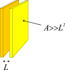
Figure 1: Original Casimir configuration of two plane parallel mirrors a distance $L$ apart.

He found an expression for the force $F_{\mathrm{Cas}}$ and the corresponding energy $E_{\mathrm{Cas}}$ which only depend on the distance $L$, the area $A$ and two fundamental constants, the speed of light $c$ and Planck constant $\hbar$

$$F_{\mathrm{Cas}} = \frac{\hbar c\pi^{2}A}{240L^{4}}=\frac{\mathrm{d}E_{\mathrm{Cas}}}{\mathrm{d}L}$$

$$E_{\mathrm{Cas}} = -\frac{\hbar c\pi^{2}A}{720L^{3}}$$ (1)

Each transverse dimension of the plates has been supposed to be much larger than $L$. Conventions of sign have been chosen so that $F_{\mathrm{Cas}}$ is positive while $E_{\mathrm{Cas}}$ is negative. They correspond to an attractive force ($\sim 0.1\mu$N for $A=1{\rm cm}^{2}$ and $L=1\mu$m) and a binding energy.

The fact that the Casimir force (1) only depends on fundamental constants and geometrical features is remarkable. In particular it is independent of the fine structure constant which appears in the expression of the atomic Van der Waals forces. This universality property is related to the assumption of perfect reflection used by Casimir in his derivation. Perfect mirrors correspond to a saturated response to the fields since they reflect 100% of the incoming light. This explains why the Casimir effect, though it has its microscopic origin in the interaction of electrons with electromagnetic fields, does not depend on the fine structure constant.

However, no real mirror can be considered as a perfect reflector at all field frequencies. In particular, the most precise experiments are performed with metallic mirrors which show perfect reflection only at frequencies smaller than a characteristic plasma frequency $\omega_{\mathrm{P}}$ which depends on the properties of conduction electrons in the metal. Hence the Casimir force between metal plates can fit the ideal Casimir formula (1) only at distances $L$ much larger than the plasma wavelength

$$\lambda_{\mathrm{P}}=\frac{2\pi c}{\omega_{\mathrm{P}}}$$ (2)

For metals used in the recent experiments, this wavelength lies in the $0.1\mu$m range (107nm for Al and 137nm for Cu and Au). At distances smaller than or of the order of the plasma wavelength, the finite conductivity of the metal has a significant effect on the force. The idea has been known since a long time Lifshitz56 ; Heinrichs75 ; Schwinger78 but a precise quantitative investigation of the effect of imperfect reflection has been systematically developed only recently Lamoreaux99 ; Lambrecht00 ; KlimPRA00 ; MostepanenkoPRA00 . As the effect of imperfect reflection is large in the most accurate experiments, a precise knowledge of its frequency dependence is essential for obtaining an accurate theoretical prediction of the Casimir force.

This is also true for other corrections to the ideal Casimir formula associated with the experimental configuration. For experiments at room temperature, the effect of thermal field fluctuations, superimposed to that of vacuum, affects the Casimir force at distances larger than a few microns. Again the idea has been known for a long time Mehra67 ; Brown69 but a quantitative evaluation taking into account the correlation of this effect with that of imperfect reflection has been mastered only recently Genet00 ; Reynaud03 . A number of publications have given rise to contradictory estimations of the Casimir force between dissipative mirrors at non zero temperature Bostrom00 ; Svetovoy00 ; Bordag00 ; Klimchitskaya01 ; Hoye03 . Many attempts have been made to elucidate the problem by taking into account the low-frequency character of the force between metallic films Lamoreaux04 , the spatial dispersion on electromagnetic surface modes Sernelius05 or the transverse momentum dependance of surface impedances Svetovoy04 ; BrevikPRE05 ; Hoye05 . Experimentally the effect of temperature of the Casimir force has not yet be conclusively measured Mostepanenko05 . For a recent analysis of this issue see reference BrevikNJP06 .

Most experiments are performed between a plane and a sphere with the force estimation involving a geometry correction. Usually the Casimir force in the plane-sphere (PS) geometry is calculated using the Proximity Force Approximation (PFA). This approximation amounts to the addition of force or energy contributions corresponding to different local inter-plate distances, assuming these contributions to be independent. But the Casimir force and energy are not additive, so that the PFA cannot be exact, although it is often improperly called a theorem.

In the present review, we consider both the original Casimir geometry with perfectly plane and parallel mirrors and the plane-sphere geometry when comparing to experiments. The PFA is expected to be valid in the plane-sphere geometry, when the sphere radius $R$ is much larger than the separation $L$ Derjaguin68 ; Langbein71 ; Kiefer78 , which is the case for all present day experiments, and it will thus be used to connect the two geometries. In this case, the force $F_{\mathrm{PS}}$ between a sphere of radius $R$ and a plane at a distance of closest approach $L$ is given in terms of the energy $E_{\mathrm{PP}}$ for the plane-plane cavity as follows

$$F_{\mathrm{PS}}=2\pi R\frac{E_{\mathrm{PP}}}{A}\quad,\quad L\ll R$$ (3)

Interesting attempts to go beyond this approximation concerning the plane-sphere geometry have been made recently JaffePRA05 ; Gies06 , in the more general context of the connection between geometry and the Casimir effect Balian78 ; Plunien86 ; Balian04 .

Another important correction to the Casimir force is coming from surface roughness, which is intrinsic to any real mirror, with amplitude and spectrum varying depending on the surface preparation techniques. The departure from flatness of the metallic plates may also be designed, in particular under the form of sinusoidal corrugation of the plates which produce a measurable lateral component of the Casimir force ChenPRL02 . For a long time, these roughness or corrugation corrections to the Casimir force have been calculated with methods valid only in limiting cases Bree74 ; Maradudin75 ; Maradudin80 ; Vesperinas82 ; EmigPRL01 ; EmigEPL03 or by using PFA BordagPLA95 ; KlimPRA99 ; BlagovPRA04 . Once again, it is only recently that emphasis has been put on the necessity of a more general method for evaluating the effect of roughness outside the region of validity of PFA with imperfect mirrors at arbitrary distances from each other GenetEPL03 . While the condition $L\ll R$ is sufficient for applying the PFA in the plane-sphere geometry, more stringent conditions are needed for PFA to hold for rough or corrugated surfaces. The surfaces should indeed be nearly plane when looked at on a scale comparable with the separation $L$, and this condition is not always satisfied in experiments. When PFA is no longer valid, the effect of roughness or corrugation can be evaluated by using the scattering theory extended to the case of non-specular reflection.

We review the Casimir effect within scattering theory and the theory of quantum optical networks. The main idea of this derivation is that the Casimir force has its origin in a difference of the radiation pressure of vacuum fields between the two mirrors and in the outer free field vacuum. This vacuum radiation pressure can be written as an integral over all modes, each mode being associated with reflection amplitudes on the two mirrors. We first present formulas written for specular reflection which are valid for losslessJaekel91 as well as lossy mirrors GenetPRA03 . We discuss the influence of the mirrors reflection coefficients at zero and non-zero temperature. We then extend the approach to the case of non-specular reflection which mixes the field polarizations and transverse wave-vectors. Finally we apply the latter approach to the calculation of the roughness correction to the Casimir force between metallic mirrors MaiaEPL05 ; MaiaPRA05 and of the lateral component of the Casimir force between corrugated plates MaiaPRL06 .

II Specular scattering

Let us first consider the original Casimir geometry with perfectly plane and parallel mirrors aligned along the directions $x$ and $y$. The two mirrors thus form a Fabry-Perot cavity of length $L$ as shown in Fig.2. We analyze the cavity as a composed optical network, and calculate the fluctuations of the intracavity fields propagating along the positive and negative $z$-axis, $\stackrel{{\scriptstyle\rightarrow}}{{\mathrm{E}}}_{\mathrm{C}}$ and $\stackrel{{\scriptstyle\leftarrow}}{{\mathrm{E}}}_{\mathrm{C}}$, in terms of the fluctuations of the incoming free-space fields $\mathrm{E}_{\mathrm{L}}^{\mathrm{in}}$ and $\mathrm{E}_{\mathrm{R}}^{\mathrm{in}}$ (the outgoing fields $\mathrm{E}_{\mathrm{L}}^{\mathrm{out}}$ and $\mathrm{E}_{\mathrm{R}}^{\mathrm{out}}$ are also shown).

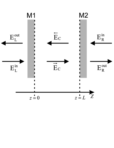
Figure 2: Schematic view of a Fabry-Perot cavity of length $L$.

The field modes are conveniently characterized by their frequency $\omega$, transverse wavevector $\mathbf{k}$ with components $k_{x},k_{y}$ in the plane of the mirrors and polarization $p$. As the configuration of Fig.2 obeys a symmetry with respect to time translation as well as transverse space translations (along directions $x$ and $y$), the frequency $\omega$, transverse vector $\mathbf{k}\equiv\left(k_{x},k_{y}\right)$ and polarization $p=\mathrm{TE},\mathrm{TM}$ are preserved throughout the whole scattering processes on a mirror or a cavity. The scattering couples only the free vacuum modes which have the same values for the preserved quantum numbers and differ by the sign of the longitudinal component $k_{z}$ of the wavevector. We denote by $\left(r_{\mathbf{k}}^{p}\left[\omega\right]\right)_{j}$ the reflection amplitude of the mirror $j=1,2$ as seen from the inner side of the cavity. This scattering amplitude obeys general properties of causality, unitarity and high frequency transparency. The additional fluctuations accompanying losses inside the mirrors are deduced from the optical theorem applied to the scattering process which couples the modes of interest and the noise modes Barnett96 ; Courty00 .

The loop functions which characterize the optical response of the cavity to an input field play an important role in the following

$$f_{\mathbf{k}}^{p}\left[\omega\right] = \frac{\rho_{\mathbf{k}}^{p}\left[\omega\right]}{1-\rho_{\mathbf{k}}^{p}\left[\omega\right]}$$

$$\rho_{\mathbf{k}}^{p}\left[\omega\right] = \left(r_{\mathbf{k}}^{p}\left[\omega\right]\right)_{1}\left(r_{\mathbf{k}}^{p}\left[\omega\right]\right)_{2}e^{2ik_{z}L}$$ (4)

$\rho_{\mathbf{k}}^{p}$ and $f_{\mathbf{k}}^{p}$ are respectively the open-loop and closed-loop functions corresponding to one round trip in the cavity. The system formed by the mirrors and fields is stable so that $f_{\mathbf{k}}^{p}$ is an analytic function of frequency $\omega$. Analyticity is defined with the following physical conditions in the complex plane

$$\omega\equiv i\xi \quad,\quad\Re\xi>0$$ (5)

$$k_{z}\equiv i\kappa\left[\omega\right]\quad,\quad \kappa\left[\omega\right]\equiv\sqrt{\mathbf{k}^{2}-\frac{\omega^{2}}{c^{2}}}\quad,\quad\Re\kappa\left[\omega\right]>0$$

The quantum numbers $p$ and $\mathbf{k}$ remain spectator throughout the discussion of analyticity. The sum on transverse wavevectors may be represented as a sum over the eigenvectors $k_{x}=2\pi q_{x}/L_{x},k_{y}=2\pi q_{y}/L_{y}$ associated with virtual quantization boxes along $x,y$ or, at the continuum limit $L_{x},L_{y}\to\infty$ with $A=L_{x}L_{y}$, as an integral

$$\sum_{\mathbf{k}} \equiv \sum_{q_{x}=-\infty}^{\infty}\sum_{q_{y}=-\infty}^{\infty}\to A\int_{-\infty}^{\infty}\frac{\mathrm{d}k_{x}}{2\pi}\int_{-\infty}^{\infty}\frac{\mathrm{d}k_{y}}{2\pi}$$ (6)

We then introduce the Airy function defined in classical optics as the ratio of energy inside the cavity to energy outside the cavity for a given mode

$$g_{\mathbf{k}}^{p}\left[\omega\right]=1+\left\{f_{\mathbf{k}}^{p}\left[\omega\right]+c.c.\right\}=\frac{1-\left|\rho_{\mathbf{k}}^{p}\left[\omega\right]\right|^{2}}{\left|1-\rho_{\mathbf{k}}^{p}\left[\omega\right]\right|^{2}}$$ (7)

$f_{\mathbf{k}}^{p}$, $g_{\mathbf{k}}^{p}$ depend only on the reflection amplitudes of mirrors as they are seen from the inner side. With these definitions we write the Casimir force

$$F = -\hbar\sum_{p}\sum_{\mathbf{k}}\int_{0}^{\infty}\frac{\mathrm{d}\omega}{2\pi}\left\{i\kappa\left[\omega\right]f_{\mathbf{k}}^{p}\left[\omega\right]+c.c.\right\}$$ (8)

or, equivalently, the Casimir energy

$$E = -\hbar\sum_{p}\sum_{\mathbf{k}}\int_{0}^{\infty}\frac{\mathrm{d}\omega}{2\pi}\frac{1}{2i}\ln\left[\frac{1-\rho_{\mathbf{k}}^{p}[\omega]}{1-\rho_{\mathbf{k}}^{p}[\omega]^{*}}\right]$$ (9)

Equations (8,9) contain the contribution of ordinary modes freely propagating outside and inside the cavity with $\omega>c|\mathbf{k}|$ and $k_{z}$ real. This contribution thus merely reflects the intuitive picture of a radiation pressure of fluctuations on the mirrors of the cavity Jaekel91 with the factor $g_{\mathbf{k}}^{p}-1$ representing a difference between inner and outer sides. Equations (8,9) also include the contribution of evanescent waves with $\omega<c|\mathbf{k}|$ and $k_{z}$ imaginary. Those waves propagate inside the mirrors with an incidence angle larger than the limit angle and they also exert a radiation pressure on the mirrors, due to the frustrated reflection phenomenon GenetPRA03 . Their properties are conveniently described through an analytical continuation of those of ordinary waves, using the well defined analytic behavior of $\kappa$ and $f_{\mathbf{k}}^{p}$.

Using analyticity properties, we now transform (8) into an integral over imaginary frequencies by applying the Cauchy theorem on the contour enclosing the quadrant $\Re\omega>0,\Im\omega>0$. We use high frequency transparency to neglect the contribution of large frequencies. This leads to the following expression for the Casimir force

$$F=\hbar\sum_{p}\sum_{\mathbf{k}}\int_{0}^{\infty}\frac{\mathrm{d}\xi}{2\pi}\left\{\kappa\left[i\xi\right]f_{\mathbf{k}}^{p}\left[i\xi\right]+c.c.\right\}$$ (10)

which is now written as an integral over complex frequencies $\omega=i\xi$. In the same way we obtain the Casimir energy as a function of imaginary frequencies

$$E=\frac{\hbar A}{2\pi}\sum_{p}\int\frac{\mathrm{d}^{2}\mathbf{k}}{4\pi^{2}}\int\limits_{0}^{\infty}\mathrm{d}\xi\ \ln\left[1-\rho_{\mathbf{k}}^{p}\left[i\xi\right]\right]$$ (11)

Causality and passivity conditions assure that the integrand $\ln\left[1-\rho_{\mathbf{k}}^{p}\left[i\xi\right]\right]$ is analytical in the upper half space of the complex plane $\Re\xi>0$. It is thus clear that both expressions for force and energy are equivalent.

II.1 Finite conductivity correction

Let us now review the correction to the Casimir force coming from the finite conductivity of any material. This correction is given by relations (8) or, equivalently, (10), as soon as the reflection amplitudes are known. These amplitudes are commonly deduced from models of mirrors, in particular bulk mirrors, slabs or layered mirrors, the optical response of metallic matter being described by some permittivity function. This function may be either a simple description of conduction electrons in terms of a plasma or Drude model or a more elaborate representation based upon tabulated optical data. At the end of the section, we will discuss the uncertainty in the theoretical evaluation of the Casimir force coming from the lack of knowledge of the specific material properties of a given mirror as was illustrated in Lambrecht00 .

Assuming that the metal plates have a large optical thickness, the reflection coefficients correspond to the ones of a simple vacuum-bulk interface LandauECM9

$$r^{\mathrm{TE}} = -\frac{\sqrt{\xi^{2}\left(\varepsilon\left(i\xi\right)-1\right)+c^{2}\kappa^{2}}-c\kappa}{\sqrt{\xi^{2}\left(\varepsilon\left(i\xi\right)-1\right)+c^{2}\kappa^{2}}+c\kappa}$$

$$r^{\mathrm{TM}} = \frac{\sqrt{\xi^{2}\left(\varepsilon\left(i\xi\right)-1\right)+c^{2}\kappa^{2}}-c\kappa\varepsilon\left(i\xi\right)}{\sqrt{\xi^{2}\left(\varepsilon\left(i\xi\right)-1\right)+c^{2}\kappa^{2}}+c\kappa\varepsilon\left(i\xi\right)}$$ (12)

$r^{p}$ stands for $r^{p}\left(i\xi,i\kappa\right)$ and $\varepsilon\left(i\xi\right)$ is the dielectric function of the metal evaluated for imaginary frequencies; the index $\mathbf{k}$ has been dropped.

Taken together, the relations (10,12) reproduce the Lifshitz expression for the Casimir force Lifshitz56 . Note that the expression was not written in this manner by Lifshitz. To our present knowledge, Kats Kats77 was the first to stress that Lifshitz expression could be written in terms of the reflection amplitudes (12). We then have to emphasize that (10) is much more general than Lifshitz expression since it still holds with mirrors characterized by reflection amplitudes differing from (12). As an illustration, we may consider metallic slabs having a finite thickness.

For a given polarization, we denote by $r_{\mathrm{si}}$ the reflection coefficient (12) corresponding to a single vacuum/metal interface and we write the reflection amplitude $r$ for the slab of finite thickness through a Fabry-Pérot formula

$$r = r_{\mathrm{si}}\frac{1-e^{-2\delta}}{1-r_{\mathrm{si}}^{2}e^{-2\delta}}$$

$$\delta = \frac{D}{c}\sqrt{\xi^{2}\left(\varepsilon\left(i\xi\right)-1\right)+c^{2}\kappa^{2}}$$ (13)

This expression has been written directly for imaginary frequencies. The parameter $\delta$ represents the optical length in the metallic slab and $D$ the physical thickness. The single interface expression (12) is recovered in the limit of a large optical thickness $\delta\gg 1$. With the plasma model, this condition just means that the thickness $D$ is larger than the plasma wavelength $\lambda_{\mathrm{P}}$.

In order to discuss experiments, it may also be worth to write the reflection coefficients for multilayer mirrors. For example one may consider two-layer mirrors with a layer of thickness $D$ of a metal $A$ deposited on a large slab of metal $B$ in the limit of large thickness as shown in Figure 3.

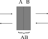
Figure 3: Composition of networks : two networks labeled A and B are piled up to build up a network AB.

The reflection formulas are then obtained as in Lambrecht97 but accounting for oblique incidence

$$r_{AB}=r_{A}+\frac{t_{A}^{2}r_{B}}{1-r_{A}r_{B}}\quad,\quad t_{AB}=\frac{t_{A}t_{B}}{1-r_{A}r_{B}}$$ (14)

It reproduces the known results for the simple multilayer systems which have already been studied Bordag01 . The combination of (13) and (14) allows to calculate most of the experimental situations precisely.

In order to assess quantitatively the effect of finite conductivity, we may in a first approach use the plasma model for the metallic dielectric function, with $\omega_{\mathrm{P}}$ the plasma frequency,

$$\varepsilon\left(\omega\right)=1-\frac{\omega_{\mathrm{P}}^{2}}{\omega^{2}}\quad,\quad\varepsilon\left(i\xi\right)=1+\frac{\omega_{\mathrm{P}}^{2}}{\xi^{2}}$$ (15)

It is convenient to present the change in the Casimir force in terms of a factor $\eta_{F}$ which measures the reduction of the force with respect to the case of perfect mirrors

$$F=\eta_{F}F_{C}$$ (16)

Using expressions (12,15) it is possible to obtain the reduction factor defined for the Casimir force through numerical integrations.

The result is plotted as the solid line on figure 4, as a function of the dimensionless parameter $\frac{L}{\lambda_{\mathrm{P}}}$, that is the ratio between the distance $L$ and the plasma wavelength $\lambda_{\mathrm{P}}$. As expected the Casimir formula is reproduced at large distances ($\eta_{F}\rightarrow 1$ when $L\gg\lambda_{\mathrm{P}}$). At distances smaller than $\lambda_{\mathrm{P}}$ in contrast, a significant reduction is obtained with the asymptotic law of variation read as GenetAFLdB04 ; Henkel04

$$L \ll \lambda_{\mathrm{P}}\quad\rightarrow\quad\eta_{F}=\alpha\frac{L}{\lambda_{\mathrm{P}}}\quad\alpha\simeq 1.193$$ (17)

This can be understood as the result of the Coulomb interaction of surface plasmons at the two vacuum/metal interfaces Kampen68 ; GenetAFLdB04 . The generalization of this idea at arbitrary distances is more subtle since it involves a full electromagnetic treatment of the plasmon as well as ordinary photon modes plasmon .

Figure 4: Reduction of the Casimir force compared to the force between perfect mirrors, when the finite conductivity is described by a plasma model (solid line) or a Drude model (dashed line) with a ratio $\frac{\gamma}{\omega_{\mathrm{P}}}$ equal to $4\times 10^{-3}$. The difference due to the relaxation parameter has only a small effect on the calculation of the Casimir force. The dotted-dashed line corresponds to the short distance asymptotic behavior (17).

The plasma model cannot provide a fully satisfactory description of the optical response of metals, in particular because it does not account for any dissipative mechanism. A more realistic representation is the Drude model AshcroftMermin

$$\varepsilon\left(\omega\right) = 1-\frac{\omega_{\mathrm{P}}^{2}}{\omega\left(\omega+i\gamma\right)}$$

$$\varepsilon\left(i\xi\right) = 1+\frac{\omega_{\mathrm{P}}^{2}}{\xi\left(\xi+\gamma\right)}$$ (18)

This model describes not only the plasma response of conduction electrons with $\omega_{\mathrm{P}}$ still interpreted as the plasma frequency but also their relaxation, $\gamma$ being the inverse of the electronic relaxation time.

The relaxation parameter $\gamma$ is much smaller than the plasma frequency. For Al, Au, Cu in particular, the ratio $\gamma/\omega_{\mathrm{P}}$ is of the order of $4\times 10^{-3}$. Hence relaxation affects the dielectric constant in a significant manner only at frequencies where the latter is much larger than unity. In this region, the metallic mirrors behave as a nearly perfect reflectors so that, finally, the relaxation does not have a large influence on the Casimir effect at zero temperature. This qualitative discussion is confirmed by the result of numerical integration reported as the dashed line on figure 4. With the typical value already given for $\gamma/\omega_{\mathrm{P}}$, the variation of $\eta_{F}$ remains everywhere smaller than 2%.

For metals like Al, Au, Cu, the dielectric constant departs from the Drude model when interband transitions are reached, that is when the photon energy reaches a few eV. Hence, a more precise description of the dielectric constant should be used for evaluating the Casimir force in the sub-$\mu$m range. This description relies on one hand on the causality relations obeyed by the dielectric response function and on another hand on known optical data. The reader is referred to Lambrecht00 for a detailed analysis, but we recall here the main argument and some important details. Let us first recall that frequencies are measured either in $e$V or in rad/s, using the equivalence 1 eV $=1.519\times 10^{15}$ rad/s. An erroneous conversion factor 1 eV $=1.537\times 10^{15}$ rad/s was used in Lambrecht00 , which led to a difference in $\varepsilon(i\xi)$ of less than 1% over the relevant distance range. In the end of the calculation, this was corresponding to a negligible error in the Casimir force and energy data .

The values of the complex index of refraction for different metals, measured through different optical techniques, are tabulated as a function of frequency in several handbooks Palik ; McGrawHill ; CRC98 . Optical data may vary from one reference to another, not only because of experimental uncertainties but also because of the dispersion of material properties of the analyzed samples. Moreover, the available data do not cover a broad enough frequency range so that they have to be extrapolated. These problems may cause variations of the results obtained for the dielectric function $\varepsilon\left(i\xi\right)$ and, therefore, for the Casimir force.

Figure 5: Dielectric function of Cu versus imaginary frequency. The solid line corresponds to the first set (optical data given by Palik ; McGrawHill , low frequencies extrapolated by a Drude model with $\omega_{\mathrm{P}}=8.97$ eV and $\gamma=29.5$ meV), the dashed line to the second set (optical data given by CRC98 , low frequencies extrapolated by a Drude model with $\omega_{\mathrm{P}}=7.5$ eV and $\gamma=130$ me V).

Figure 5 shows two different plots of $\varepsilon\left(i\xi\right)$ for Cu as a function of imaginary frequency $\xi$. The solid line corresponds to the first data set with data points taken from Palik ; McGrawHill and extrapolation at low frequency with a Drude model with parameters $\omega_{\mathrm{P}}=8.97$ eV and $\gamma=29.5$ meV in reasonable agreement with existing knowledge from solid state physics. However, as explained in Lambrecht00 , the optical data available for Cu do not permit an unambiguous estimation of the two parameters $\omega_{\mathrm{P}}$ and $\gamma$ separately. Other couples of values can be chosen which are also consistent with optical data. To make this point explicit, we have drawn a second plot on figure 5 (dashed line) with data taken from CRC98 and the low frequency interpolation given by a Drude model with $\omega_{\mathrm{P}}=7.5$ eV and $\gamma=130$ meV. These values lead to a dielectric function $\varepsilon(i\xi)$ smaller than in the first data set over the whole frequency range, but especially at low frequencies. An estimation of the uncertainties associated with this imperfect knowledge of optical data can be drawn from the computation of the Casimir force in these two cases.

Figure 6: Reduction factor $\eta_{F}$ for the Casimir force between two Cu plates as a function of the plate separation $L$. The solid line corresponds to the first set (optical data given by Palik , low frequencies extrapolated by a Drude model with $\omega_{\mathrm{P}}=8.97$ eV and $\gamma=29.5$ meV), the dashed line to the second set (optical data given by CRC98 , low frequencies extrapolated by a Drude model with $\omega_{\mathrm{P}}=7.5$ eV and $\gamma=130$ m$e$V).

Figure 6 shows the reduction factor $\eta_{F}$ for the Casimir force between two Cu plates as a function of the plate separation $L$ for the two sets of optical data. The two corresponding curves have similar dependance on the plate separation but the absolute values are shifted from one curve to the other. At a separation of 100 nm the difference can be as large as 5%. As the plasma frequency is basically the frequency above which the mirrors reflectivity diminishes considerably, the Drude parameters of the first set ($\omega_{\mathrm{P}}=8.97$ eV and $\gamma=29.5$ meV) give a larger Casimir force than the second set, where the plasma frequency is lower ($\omega_{\mathrm{P}}=7.5$ eV and $\gamma=130$ meV). A detailed analysis of this uncertainty has been recently reported Pirozhenko06 .

Let us emphasize that the problem here is neither due to a lack of precision of the calculations nor to inaccuracies in experiments. The problem is that calculations and experiments may consider physical systems with different optical properties. Material properties of mirrors indeed vary considerably as a function of external parameters and preparation procedure Pirozhenko06 . This difficulty could be solved by measuring the reflection amplitudes of the mirrors used in the experiment and then inserting these informations in the formula giving the predicted Casimir force. In order to suppress the uncertainty associated with the extrapolation procedure, it would be necessary to measure the reflection amplitudes down to frequencies of the order of 1 meV, if the aim is to calculate the Casimir force in the distance range from 100 nm to a few $\mu$m.

II.2 Temperature correction

The Casimir force between dissipative metallic mirrors at non zero temperature has given rise to contradictory claims which have raised doubts about the theoretical expression of the force. In order to contribute to the resolution of this difficulty, we now review briefly the derivation of the force from basic principles of the quantum theory of lossy optical cavities at non zero temperature. We obtain an expression which is valid for arbitrary mirrors, including dissipative ones, characterized by frequency dependent reflection amplitudes. This expressions coincides with the usual Lifshitz expression when the plasma model is used to describe the mirrors material properties, but it differs when the Drude model is applied. The difference can be traced back to the validity of Poisson summation formula Reynaud03 .

To discuss the effect of finite temperature we use a theorem which gives the commutators of the intracavity fields as the product of those well known for fields outside the cavity by the Airy function. This theorem was demonstrated with an increasing range of validity in Jaekel91 , Barnett98 and GenetPRA03 . It is true regardless of whether the mirrors are lossy or not. Since it does not depend on the state of the field, it can be used for thermal as well as vacuum fluctuations. Assuming thermal equilibrium, the theorem leads to the expression of the field anticommutators, i.e. the field fluctuations. Note that thermal equilibrium has to be assumed for the whole system, which means that input fields as well as fluctuations associated with electrons, phonons and any loss mechanism inside the mirrors correspond to the same temperature $T$, whatever their microscopic origin may be. If parts of the system correspond to different temperatures, completely different results are obtained Antezza05 ; Henkel02 .

The anticommutators of intracavity fields are given by those known for fields outside the cavity multiplied by the Airy function. Hence, the expression written in GenetPRA03 for a null temperature is only modified through the appearance of a thermal factor in the integrand

$$F = -\hbar\sum_{p,\mathbf{k}}\int_{0}^{\infty}\frac{\mathrm{d}\omega}{2\pi}\left\{i\kappa_{\mathbf{k}}\left[\omega\right]f_{\mathbf{k}}^{p}\left[\omega\right]c\left[\omega\right]+c.c.\right\}$$ (19)

$$c\left[\omega\right]\equiv\coth\left(\frac{\pi\omega}{\omega_{\mathrm{T}}}\right)\quad,\quad\omega_{\mathrm{T}}\equiv\frac{2\pi k_{\mathrm{B}}T}{\hbar}$$

Using as before analyticity properties, we transform (19) into an integral over imaginary frequencies giving the following expression for the Casimir force

$$F=\hbar\sum_{p,\mathbf{k}}\int_{0}^{\infty}\frac{\mathrm{d}\xi}{2\pi}\left\{\kappa\left[i\xi+\eta\right]f_{\mathbf{k}}^{p}\left[i\xi+\eta\right]c\left[i\xi+\eta\right]+c.c.\right\}$$ (20)

It is now written as an integral over complex frequencies $\omega=i\xi+\eta$ close to the imaginary axis, with the small positive real number $\eta\to 0^{+}$ maintaining the Matsubara poles $\omega_{m}=im\omega_{\mathrm{T}}$ of $c\left[\omega\right]$ outside the contour used to apply the Cauchy theorem. Up to this point, the present derivation is similar to Lifshitz’ demonstration Lifshitz56 while being valid for arbitrary reflection amplitudes. The next steps in Lifshitz’ derivation, scrutinized in Reynaud03 , may raise difficulties for dissipative mirrors. Let us briefly recall the main arguments of Reynaud03 .

We may first write a series expansion of the Casimir force (19) based upon the expansion of the function $\coth\left(\frac{\pi\omega}{\omega_{\mathrm{T}}}\right)$ into a series of exponentials $\exp\left(-\frac{2n\pi\imath\xi}{\omega_{\mathrm{T}}}\right)$ (see also Genet00 ). This expansion obeys the mathematical criterion of uniform convergence so that, when it is inserted in (19), the order of the summation over $n$ and integration over $\xi$ may be exchanged. It follows that the force (19) may also be read as

$$F = \frac{\hbar}{\pi}\sum_{p}\sum_{\mathbf{k}}\sum_{n}^{\prime}\widetilde{\phi}_{\mathbf{k}}^{p}\left(\frac{2n\pi}{\omega_{\mathrm{T}}}\right)$$ (21)

$$\widetilde{\phi}_{\mathbf{k}}^{p}\left(x\right) \equiv 2\int_{0}^{\infty}\mathrm{d}\xi\cos\left(\xi x\right)\phi_{\mathbf{k}}^{p}\left[\xi\right]$$

$$\phi_{\mathbf{k}}^{p}\left[\xi\right] \equiv \lim_{\eta\to 0^{+}}\kappa_{\mathbf{k}}\left[i\xi+\eta\right]f_{\mathbf{k}}^{p}\left[i\xi+\eta\right]$$

We have introduced the common summation convention

$$\sum_{n}^{\prime}\varphi\left(n\right)\equiv\frac{1}{2}\varphi\left(0\right)+\sum_{n=1}^{\infty}\varphi\left(n\right)$$ (22)

The function $\phi_{\mathbf{k}}^{p}$ is well defined almost everywhere, the only possible exception being the point $\xi=0$ where the limit $\eta\to 0^{+}$ may be ill defined for mirrors described by dissipative optical models Klimchitskaya01 . Since this is a domain of null measure, the cosine Fourier transform $\widetilde{\phi}_{\mathbf{k}}^{p}$ of $\phi_{\mathbf{k}}^{p}$ is well defined everywhere and the expression (21) of the Casimir force is valid for arbitrary mirrors, including dissipative ones. Note that the term $n=0$ in (21) corresponds exactly to the contribution of vacuum fluctuations, or to the zero temperature limit, while the terms $n\geq 1$ give the corrections associated with thermal fields.

We come back to the derivation of the Lifshitz formula Lifshitz56 , often used as the standard expression of the Casimir force. This formula is directly related to the decomposition of the $\coth$ function into elementary fractions corresponding to the Matsubara poles $\Omega_{m}=im\omega_{\mathrm{T}}$. If we assume furthermore that the function $\phi_{\mathbf{k}}^{p}$ is a sufficiently smooth test function, in the sense defined by the theory of distributions, we deduce that the expression (20) can also be read

$$F_{\mathrm{Lif}}=\frac{\hbar\omega_{\mathrm{T}}}{\pi}\sum_{p}\sum_{\mathbf{k}}\sum_{m}^{\prime}\phi_{\mathbf{k}}^{p}\left[m\omega_{\mathrm{T}}\right]$$ (23)

This is the generalization of the Lifshitz’ formula Lifshitz56 to the case of arbitrary reflection amplitudes. It is a discrete sum over Matsubara poles with the primed summation symbol having the definition (22). This formula is known to lead to the correct result in the case of dielectric mirrors (for which it was derived in Lifshitz56 ), for perfect mirrors Mehra67 ; Brown69 and also for metallic mirrors described by the lossless plasma model Genet00 .

However its applicability to arbitrary mirrors remains a matter of controversy Klimchitskaya01 . The point is that the derivation of the Lifshitz’ formula (23) requires that the function $\phi_{\mathbf{k}}^{p}$ be a sufficiently smooth test function, in the sense defined by the theory of distributions. Whether or not this is the case at $\xi=0$ for $\phi_{\mathbf{k}}^{p}$ calculated from dissipative optical models constitutes the central question of the controversy on the value of the term $p$=TE, $m=0$ in Lifshitz’ sum Bostrom00 ; Svetovoy00 ; Bordag00 ; Klimchitskaya01 ; Hoye03 . Let us repeat that (21) is still a mathematically valid expression of the Casimir force even when $\phi_{\mathbf{k}}^{p}$ is ill defined for $\xi$ in a domain of null measure. The question of validity of Lifshitz’ formula (23) may also be phrased in terms of applicability of the Poisson summation formula MorseFeshbach . This applicability depends on a smoothness condition which is met for dielectric mirrors, for perfect mirrors and for mirrors described by the plasma model and this explains why Lifshitz’ formula (23) may be used as well as (21) in these cases Reynaud03 .

In order to solve this controversy, it is crucial to improve our knowledge of the reflection amplitudes at low frequencies. As already discussed, the best manner to do that is to measure these amplitudes on the mirrors used in the experiment at frequencies as low as possible. Although the theoretical question of a good modeling of mirrors at low frequencies is certainly of interest and needs to be answered, the crucial point for a reliable theory-experiment comparison is the necessity of assessing the real behavior of the mirrors used in the experiments.

III Non specular scattering

We will now present a more general formalism to calculate the Casimir force and energy which takes into account non-specular reflection by the plates. Non-specular reflection is of course the generic reflection process on any mirror while specular reflection is an idealization.

In order to introduce the more general formula, let us first rewrite expression (11) of the Casimir energy between two flat plates as a sum over modes labeled by the $\xi$ and $m\equiv\mathbf{k},p$

$$E_{\mathrm{sp}}=\hbar\int\limits_{0}^{\infty}\frac{\mathrm{d}\xi}{2\pi}\mathrm{Tr}\Delta_{\mathbf{k}}^{p}\left[i\xi\right]$$

$$\Delta_{\mathbf{k}}^{p}\left[i\xi\right]=\ln\left(1-r_{1}r_{2}e^{-2\kappa L}\right)$$ (24)

This can be interpreted as the energy stored inside the cavity during the scattering process. It is expressed in terms of the phase shifts $\Delta_{\mathbf{k}}^{p}\left[i\xi\right]$ acquired by the field modes upon scattering on the cavity. These phase shifts are deduced from the $S$-matrix of the cavity Jaekel91 in such a manner that the Casimir energy is simply equal to the logarithm of the determinant of the $S-$matrix. Using the techniques of quantum field theory Plunien86 , this can also be written as the trace of matrix, here diagonal, defined on these modes

$$E_{\mathrm{sp}}=\hbar\int\limits_{0}^{\infty}\frac{\mathrm{d}\xi}{2\pi}\sum_{m}\left\langle m\right|\ln(1-r_{1}r_{2}e^{-2\kappa_{i}L})\left|m\right\rangle$$ (25)

Here, $r_{1}$ and $r_{2}$ are diagonal matrices which contain as their diagonal elements the specular reflection amplitudes, as they are seen from fields inside the cavity,

$$\left\langle m\right|r_{i}\left|m^{\prime}\right\rangle\equiv\delta_{m,m^{\prime}}~{}r_{i}\left(\xi,m\right)$$

$$\delta_{m,m^{\prime}}\equiv 4\pi^{2}\delta\left(\mathbf{k}-\mathbf{k}^{\prime}\right)\delta_{p,p^{\prime}}$$ (26)

while $\kappa$ is a matrix diagonal over the same modes

$$\left\langle m\right|\kappa\left|m^{\prime}\right\rangle\equiv\sqrt{\mathbf{k}_{m}^{2}+\xi^{2}}\delta_{m,m^{\prime}}$$ (27)

It is now easy to write down a more general formula of the Casimir energy for the case of stationary but non-specular scattering

$$E_{\mathrm{nsp}}=\hbar\int\limits_{0}^{\infty}\frac{\mathrm{d}\xi}{2\pi}\mathrm{Tr}\ln\left(1-\mathcal{R}_{1}e^{-\kappa L}\mathcal{R}_{2}e^{-\kappa L}\right)$$ (28)

The two matrices $\mathcal{R}_{1}$ and $\mathcal{R}_{2}$ are no longer diagonal on plane waves since they describe non specular reflection on the two mirrors. The propagation factors remain diagonal on plane waves. Note that the matrices appearing in (28) no longer commute with each other. As a consequence, the two propagation matrices in (28) can be moved through circular permutations in the product but not adjoined to each other.

Formula (28) has already been used to evaluate the effect of roughness MaiaEPL05 ; MaiaPRA05 or corrugation MaiaPRL06 of the mirrors on the Casimir force. To this aim, it was expanded at second order in the profiles of the mirrors, with the optical response of the bulk metals described by the plasma model. The non specular reflection amplitudes were then deduced from techniques developed for treating rough plates Agarwal77 ; Greffet88 . The condition of validity of this expansion is that the roughness or corrugation amplitude is the smallest of length scales involved in the problem. In this regime, it was possible to investigate various domains for the roughness or corrugation wavelength and thus to investigate the effect of roughness or corrugation outside as well as inside the range of validity of the Proximity Force Approximation.

We may again emphasize at this point that the formula (28) has a wider range of validity than used in those applications. It can in principle describe mirrors with nanostructured surfaces corresponding to large amplitudes which cannot be treated as a small perturbation. It can as well deal with more complicated optical responses which are described neither by a plasma nor by a Drude model. As was extensively discussed above for the case of specular reflection, the formula (28) remains valid for arbitrary mirrors, the only problem being to obtain the precise form of the reflection matrices to be inserted into it.

III.1 Influence of surface roughness

Let us now recall how the non-specular scattering formula (28) can be used to calculate the effect of roughness on the Casimir force. Taking this effect into account simultaneously with that of finite conductivity is essential, because both of them are important at short distances. In order to analyze the roughness effect between two metallic plates, we will describe the optical properties of the mirrors by the plasma model. The values for the plasma wavelength, the mirror separation and the roughness correlation length will be arbitrary with respect to each other, the roughness amplitude remaining the smallest length scale for perturbation theory to hold. We will review some simple analytical expressions for several limiting cases, as well as numerical results allowing one for a reliable calculation of the roughness correction in real experiments MaiaEPL05 ; MaiaPRA05 .

In a plane-plane geometry, the surface profiles are defined by the functions $h_{i}(x,y)$ $(i=1,2)$ giving the local heights with respect to the mean separation $L$ along the $z$ direction as shown in Fig.7.

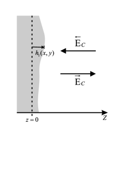
Figure 7: Magnified detail of the internal surface of mirror M1.

These functions are defined so that they have zero averages. We consider the case of stochastic roughness characterized by spectra

$$\sigma_{ij}(\mathbf{k})=\int\mathrm{d}^{2}\mathbf{r}\,e^{-i\mathbf{k}\cdot\mathbf{r}}\langle h_{i}(\mathbf{r})\,h_{j}(\mathbf{0})\rangle\;,\quad i=1,2$$ (29)

We suppose the surface $A$ of the plates to contain many correlation areas, which allows us to take ensemble or surface averages interchangeably. The two plates are considered to be made of the same metal and the crossed correlation between their profiles is neglected ($\sigma_{12}(\mathbf{k})=0$).

We obtain the following variation of the Casimir energy $E_{PP}$ up to second order in the perturbations $h_{i}$ GenetEPL03

$$\delta E_{\rm PP}=\int\frac{\mathrm{d}^{2}\mathbf{k}}{4\pi^{2}}G_{\mathrm{r}}(\mathbf{k})\sigma(\mathbf{k})$$ (30)

$$\sigma(\mathbf{k})=\sigma_{11}(\mathbf{k})+\sigma_{22}(\mathbf{k})$$

With our assumptions, the spectrum $\sigma(\mathbf{k})$ fully characterizes the roughness of the two plates. The correlation length $\ell_{C}$ is defined as the inverse of its width. The response function $G_{\mathrm{r}}(\mathbf{k})$ then describes the spectral sensitivity to roughness of the Casimir effect. Symmetry requires that it only depends on $k=|\mathbf{k}|$. The dependance of $G_{\mathrm{r}}$ on $k$ reflects that not only the roughness amplitude but also its spectrum plays a role in diffraction on rough surfaces Agarwal77 ; Greffet88 . The formula (30) has been obtained for the energy in the plane-plane configuration but it also determines the force correction $\delta F_{\mathrm{PS}}$ in the plane-sphere configuration since the PFA is still used for describing the weak curvature of the sphere (see below).

We now focus our attention on the validity of PFA for treating the effect of roughness and notice that this validity only holds at the limit of smooth surface profiles $k\to 0$. In fact, the following identity is obeyed by our result MaiaEPL05 , for arbitrary values of $L$ and $\lambda_{\mathrm{P}}$,

$$G_{\mathrm{r}}\left(k\to 0\right)=\frac{E_{\mathrm{PP}}^{\prime\prime}(L)}{2}$$ (31)

where the derivative is taken with respect to the plate separation $L$. If we now suppose that the roughness spectrum $\sigma(k)$ is included inside the PFA sector where $G_{\mathrm{r}}\left(k\right)\simeq G_{\mathrm{r}}\left(0\right)$, $G_{\mathrm{r}}$ may be replaced by $G_{\mathrm{r}}(0)$ and factored out of the integral (30) thus leading to the PFA expression GenetEPL03

$$\delta E_{\mathrm{PP}}=\frac{E^{\prime\prime}_{\mathrm{PP}}(L)}{2}a^{2}$$ (32)

$$a^{2}=\int\frac{\mathrm{d}^{2}\mathbf{k}}{4\pi^{2}}\sigma(\mathbf{k})\equiv\langle h_{1}^{2}+h_{2}^{2}\rangle$$

In this PFA limit, the correction depends only on the variance $a^{2}$ of the roughness profiles, that is also the integral of the roughness spectrum.

In the general case in contrast, the sensitivity to roughness depends on the wavevector $k$. This key point is emphasized by introducing a new function $\rho_{\mathrm{r}}(k)$ which measures the deviation from the PFA GenetEPL03

$$\rho_{\mathrm{r}}(k)=\frac{G_{\mathrm{r}}(k)}{G_{\mathrm{r}}(0)}.$$ (33)

This function is plotted on Fig. 8 for several values of $L$. As for all numerical examples considered below, we take $\lambda_{\mathrm{P}}=137$nm which corresponds to gold covered plates.

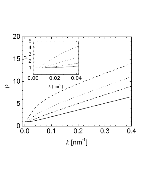
Figure 8: Variation of $\rho_{\mathrm{r}}$ versus $k$ for $L$=50, 100, 200, 400 nm (from bottom to top curve).

The ratio $\rho_{\mathrm{r}}(k)$ is almost everywhere larger than unity, which means that the PFA systematically underestimates the roughness correction. The inlet shows $\rho_{\mathrm{r}}(k)$ for small values of $k$ where the PFA is a good approximation. To give a number illustrating the deviation from the PFA, we find $\rho_{\mathrm{r}}\simeq 1.6$ for $L=200$nm and $k=0.02{\rm nm}^{-1}$, which means that the exact correction is $60\%$ larger than the PFA result for this intermediate separation and a typical roughness wavelength $2\pi/k\simeq 300$nm.

Fig. 8 indicates that $\rho_{\mathrm{r}}(k)$ grows linearly for large values of $k$. This is a general prediction of our full calculations MaiaEPL05 , for arbitrary values of $L$ and $\lambda_{\mathrm{P}}$,

$$\rho_{\mathrm{r}}(k)=\alpha_{\mathrm{r}}\,k\quad{\rm for}\quad k\gg{2\pi\over\lambda_{\mathrm{P}}}\;,\;{1\over L}$$ (34)

The dimensionless parameter $\alpha_{\mathrm{r}}/L$ depends on $2\pi L/\lambda_{P}$ only, and its expression is given by equation (8) in MaiaEPL05 . In Fig. 9, we plot the coefficient $\alpha_{\mathrm{r}}$ as a function of $L$ with $\lambda_{\mathrm{P}}=137$nm. In the limit of short distances, we recover the expression which was drawn in GenetEPL03 from older calculations Maradudin80 (after a correction by a global factor 2)

$$\alpha_{\mathrm{r}}=0.4492L\quad{\rm for}\quad k^{-1}\ll L\ll{\lambda_{\mathrm{P}}\over 2\pi}$$ (35)

In the opposite limit of large distances, the coefficient $\alpha_{\mathrm{r}}$ is found to saturate MaiaEPL05

$$\alpha_{\mathrm{r}}=\frac{14}{15}{\lambda_{\mathrm{P}}\over 2\pi}\quad{\rm for}\quad k^{-1}\ll{\lambda_{\mathrm{P}}\over 2\pi}\ll L$$ (36)

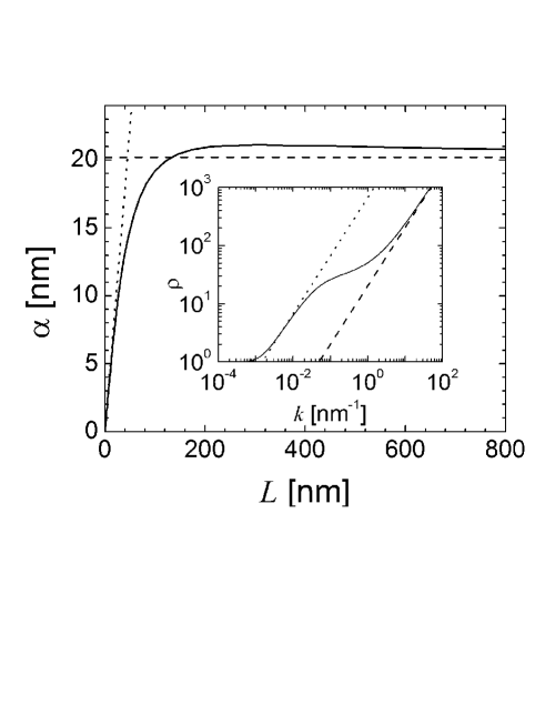
Figure 9: Variation of the coefficient $\alpha_{\mathrm{r}}$ versus $L$. The analytical result for $k^{-1}\ll L\ll\lambda_{\mathrm{P}}$ is shown as the dotted line and for $k^{-1}\ll\lambda_{\mathrm{P}}\ll L$ as the dashed line. A comparison between this second result (dashed straight line) and the exact $\rho_{\mathrm{r}}(k)$ (solid line) is shown in the inlet for $L=2\mu$m. The analytical result $\rho_{\mathrm{r}}=Lk/3$ predicted by the model of perfect reflectors (dotted line) is valid only in the intermediate range $\lambda_{\mathrm{P}}\ll k^{-1}\ll L$.

It is interesting to note that this result differs from the long distance behavior which was drawn in GenetEPL03 from the reanalysis of calculations of the effect of sinusoidal corrugations on perfectly reflecting plates EmigPRL01 . Perfect reflectors indeed correspond to the limiting case where $\lambda_{\mathrm{P}}$ rather than $1/k$ is the shortest length scale. The following result is obtained in this case MaiaEPL05 , which effectively fits that of  EmigPRL01 ,

$$\rho_{\mathrm{r}} = \frac{1}{3}L\,k\quad{\rm for}\quad\lambda_{P}\ll k^{-1}\ll L$$ (37)

The long-distance behavior is thus given by (36) when $1/k\ll\lambda_{P}\ll L$ but by (37) when $\lambda_{P}\ll 1/k\ll L$. The cross-over between these two regimes is shown in the inlet of Fig. 9, where we plot $\rho_{\mathrm{r}}$ as a function of $k$ for $L=2\mu$m. The failure of the perfect reflection model for $1/k\ll\lambda_{\mathrm{P}}$ has been given an interpretation in MaiaEPL05 : it results from the fact that not only the incoming field mode but also the outgoing one have to see the mirror as perfectly reflecting for formula (37) to be valid.

These numerical results can be used to assess the accuracy of the PFA applied to the problem of roughness. PFA is indeed recovered at the limit of very smooth surface profiles and the deviation from PFA given by our results as soon as the roughness wavevector goes out of this limit. The mirrors used in a given experiment have a specific roughness spectrum which can, and in our opinion must be, measured when the experiments are performed. The integral (30) then leads to a reliable prediction for the roughness correction, as soon as the spectral sensitivity $G_{\mathrm{r}}(k)$ and the real spectrum $\sigma(k)$ are inserted into it.

III.2 Lateral Casimir force component

The spectral sensitivity $G_{\mathrm{r}}(k)$ involved in the calculation of the roughness correction can be considered as a further prediction of Quantum ElectroDynamics, besides the more commonly studied mean Casimir force, so that the comparison of its theoretical expectation with experiments is an interesting prospect. But this comparison can hardly rely on the roughness correction (30) which remains in any case a small variation of the longitudinal Casimir effect. A more stringent test can be performed by studying the lateral component of the Casimir force which arises between corrugated surfaces. This lateral Casimir force would indeed vanish in the absence of surface corrugation so that the expression of the spectral sensitivity will thus appear directly as a factor in front of the lateral Casimir force. For reasons which will become clear below, the spectral sensitivity involved in the calculation of corrugation effect is a different function $G_{\mathrm{c}}(k)$.

Nice experiments have shown the lateral Casimir force to be measurable at separations of a few hundred nanometers ChenPRL02 , that is of the same order of magnitude as the plasma wavelength $\lambda_{\mathrm{P}}$. It follows that these experiments can neither be analyzed by assuming the mirrors to be perfect reflectors EmigEPL03 , nor by using the opposite limit of plasmon interaction Maradudin80 . It is no more possible to use the PFA if we want to be able to treat arbitrary values of the ratio of the corrugation wavelength $\lambda_{\mathrm{C}}$ to the interplate distance $L$. This is why we emphasize the results drawn from the non-specular scattering formula (28) which can be used for calculating the lateral Casimir force for arbitrary relative values of $\lambda_{\mathrm{P}}$, $\lambda_{\mathrm{C}}$ and $L$. The only drawback of this calculation is that it is restricted to small enough corrugation amplitudes, since the latter have to remain the smallest length scale for perturbation theory to hold. But the lateral force is known to be experimentally accessible in this regime. Again we model the optical response of the metallic plates by the plasma model.

The surface profiles of the corrugated plates are defined by two functions $h_{i}(\mathbf{r})$, with $\mathbf{r}=(x,y)$ is the lateral position along the surfaces of the plates while $i=1,2$ labels the two plates. As in experiments ChenPRL02 , we consider the simple case of uniaxial sinusoidal corrugations imprinted on the two plates (see Fig.10) along the same direction, say the $y$ direction, and with the same wavevector $k\equiv 2\pi/\lambda_{\mathrm{C}}$

$$h_{1}=a_{1}\cos\left(kx\right)\quad,\quad h_{2}=a_{2}\cos\left(k(x+b)\right)$$ (38)

Both profiles $h_{1}$ and $h_{2}$ have zero spatial averages and they are counted as positive when they correspond to local length decreases below the mean value $L$.

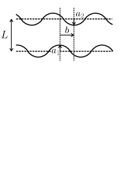
Figure 10: Surface profiles considered for the lateral component of the Casimir force. Both surfaces have a sinusoidal corrugation with $a_{1}$ and $a_{2}$ being the corrugation amplitudes, $b$ the mismatch between the two sinusoidal functions.

For the purpose of the calculation of the lateral Casimir force, the non-specular reflection matrix ${\cal R}_{j}$ have to be developed up to the first order in the deviations $h_{j}$ from flatness of the two plates. They are thus written as the sum of a zero-th order contribution identifying to the specular reflection amplitude and of a first-order contribution proportional to the Fourier component at wavevector $(\mathbf{k}-\mathbf{k}^{\prime})$ of the surface profiles, this Fourier component being able to induce a scattering of the field modes from the wavevector $\mathbf{k}$ to $\mathbf{k}^{\prime}$  MaiaPRL06 . The correction of the Casimir energy $\delta E_{\mathrm{PP}}$ induced by the corrugations arises at second order in the corrugations, with crossed terms of the form $a_{1}\,a_{2}$ which have the ability to induce lateral forces. In other words, the corrugation sensitivity function $G_{\mathrm{c}}(k)$ obtained below depends on the crossed correlation between the profiles of the two plates, in contrast to the function $G_{\mathrm{r}}(k)$ calculated above for describing the roughness spectral sensitivity. The latter were depending on terms quadratic in $h_{1}$ or $h_{2},$ and their evaluation required that second order non specular scattering be properly taken into account. Here, first order non specular amplitudes evaluated on both plates are sufficient.

The result of the calculation is read as a second-order correction induced by corrugations

$$\delta E_{\mathrm{PP}}=2\int\frac{\mathrm{d}^{2}\mathbf{k}}{(2\pi)^{2}A}{G_{\mathrm{c}}}(\mathbf{k})H_{1}(\mathbf{k})H_{2}(-\mathbf{k})$$ (39)

with the function $G_{\mathrm{c}}(\mathbf{k})$ given by equation (3) in MaiaPRL06 . For isotropic media, symmetry requires ${G_{\mathrm{c}}}(\mathbf{k})$ to depend only on the modulus of the wavevector $k=|\mathbf{k}|$. We may also assume for simplicity that the two plates are made of the same metallic medium. The energy correction thus depends on the lateral mismatch $b$ between the corrugations of the two plates, which is the cause for the lateral force to arise. Replacing the ill-defined $(2\pi)^{2}\delta^{(2)}(0)$ by the area $A$ of the plates, we derive from (39)

$$\delta E_{\mathrm{PP}}=a_{1}a_{2}\cos(kb)G_{\mathrm{c}}(k)$$ (40)

Once again, the result of the PFA is recovered from equation (40) as the limiting case $k\rightarrow 0$, that is also for long corrugation wavelengths. This corresponds to nearly plane surfaces where the Casimir energy can be obtained from the energy $E_{\mathrm{PP}}$ calculated between perfectly plane plates by averaging the ‘local’ distance ${\cal L}=L-h_{1}-h_{2}$ over the surface of the plates. Expanding at second order in the corrugation amplitudes and disregarding squared terms in $a_{1}^{2}$ and $a_{2}^{2}$ because they cannot produce a lateral dependence, we thus recover expression (40) with $G_{\mathrm{c}}(k)$ replaced, for small values of $k$ or equivalently large values of $\lambda_{\mathrm{C}}$, by $G_{\mathrm{c}}(0)$ given by (compare with (31))

$${G_{\mathrm{c}}}(k\to 0)={E_{\mathrm{PP}}^{\prime\prime}\over 2}$$ (41)

This property is ensured, for any specific model of the material medium, by the fact that $G_{\mathrm{c}}$ is given by the specular limit of non specular reflection amplitudes MaiaPRL06 for $k\rightarrow 0$. For arbitrary values of $k$, the deviation from PFA is then described by the ratio

$$\rho_{\mathrm{c}}(k)=\frac{G_{\mathrm{c}}(k)}{G_{\mathrm{c}}(0)}$$ (42)

In the following, we discuss explicit expressions of this ratio $\rho_{\mathrm{c}}$ given by its general expression (eq. (3) in MaiaPRL06 ). For the numerical examples, we take $\lambda_{\mathrm{P}}=137$nm, corresponding to gold covered plates. The result $\rho_{\mathrm{c}}$ is plotted on Fig. 11 as a function of $k$, for different values of the distance $L$.

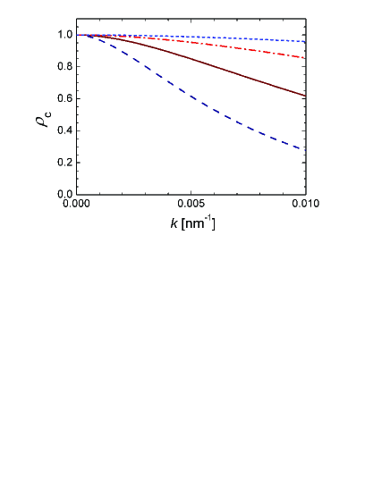
Figure 11: Variation of $\rho_{\mathrm{c}}$ versus $k$ with $\lambda_{\mathrm{P}}=137$nm and for $L=$ 50nm (dotted line), 100nm (dash-dotted line), 200nm (solid line) and 400nm (dashed line).

For example for a distance $L=50$nm, the Proximity Force Approximation is correct in the range $k\leq 0.01{\rm nm}^{-1}$ (i.e. $\lambda_{\mathrm{C}}\geq 628$nm) covered by the plot in Fig. 11. However, for typical separations of 100nm or larger, $\rho_{\mathrm{c}}$ drops significantly below its PFA value of unity. A more detailed discussion can be found in MaiaPRL06 .

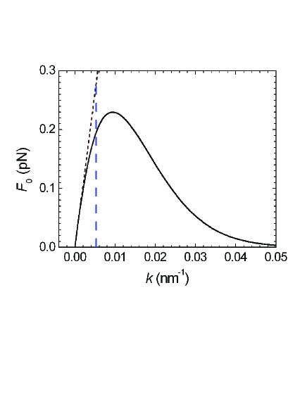
Figure 12: Lateral force amplitude for the plane-sphere setup, as a function of $k,$ with figures taken from ChenPRL02 . The experimental value $k=0.0052{\rm nm}^{-1}$ is indicated by the vertical dashed line.

For still larger values of $kL$, the functions $G_{\mathrm{c}}(k)$ and $\rho_{\mathrm{c}}(k)$ decay exponentially to zero. If we also assume that $k\lambda_{\mathrm{P}}\gg 1$, we find $G_{\mathrm{c}}(k)=\alpha_{\mathrm{c}}\,k\,\exp(-kL)$ where the parameter $\alpha_{\mathrm{c}}$ now depends on $\lambda_{\mathrm{P}}$ and $L$ only. This is in striking contrast with the behavior of the response function for stochastic roughness, which grows linearly with $k$ for large $k$ due to the contribution of the second-order reflection coefficients MaiaPRA05 . These coefficients do not contribute to the second-order lateral effect, which is related to two first-order non-specular reflections at different plates, separated by a one-way propagation with a modified momentum of the order of $k$. The resulting propagation factor is, in the large-$k$ limit, $\exp(-\kappa L)\approx\exp(-kL)$, thus explaining the exponential behavior.

III.3 Comparison to experiments in a plane-sphere configuration

In order to compare the theoretical expression of the lateral Casimir force to experiments, we have to consider the plane-sphere (PS) geometry ChenPRL02 rather than the plane-plane (PP) one. As $R\gg L$, we use the PFA to connect the two geometries. Any interplay between curvature and corrugation is avoided provided that $RL\gg\lambda_{\mathrm{C}}^{2}$. These two conditions are met in the experiment reported in ChenPRL02 , where $R=100\mu$m, $\lambda_{\mathrm{C}}=1.2\mu$m and $L\sim 200$nm.

We thus obtain the energy correction $\delta E_{\mathrm{PS}}$ between the sphere and a plane at a distance of closest approach $L$ as an integral of the energy correction $\delta E_{\mathrm{PP}}$ in the PP geometry

$$\delta E_{\mathrm{PS}}(L,b)=\int_{\infty}^{L}\frac{2\pi R\mathrm{d}L^{\prime}}{A}\delta E_{\mathrm{PP}}(L^{\prime},b)$$ (43)

Then the lateral force is deduced by varying the energy correction (43) with respect to the lateral mismatch $b$ between the two corrugations. Simple manipulations then lead to the lateral Casimir force in the PS geometry

$$F^{\mathrm{lat}}_{\mathrm{PS}}=\frac{2\pi a_{1}a_{2}}{A}kR\sin(kb)\int_{\infty}^{L}\mathrm{d}L^{\prime}G_{\mathrm{c}}(k,L^{\prime})$$ (44)

The force attains a maximal amplitude for $\sin(kb)=\pm 1$, which is easily evaluated in the PFA regime $k\rightarrow 0$ where ${G_{\mathrm{c}}}(k)$ does not depend on $k$, so that $F^{\mathrm{lat}}_{\mathrm{PS}}$ scales as $k.$ As $k$ increases, the amplitude increases at a slower rate and then starts to decrease due to the exponential decay of ${G_{\mathrm{c}}}(k)$. For a given value of the separation $L$, the lateral force reaches an optimum for a corrugation wavelength such that $kL$ is of order of unity, which generalizes the result obtained for perfect reflectors in EmigPRL01 . In Fig. 12, we plot the force $F^{\mathrm{lat}}_{\mathrm{PS}}$ (for $\sin(kb)=1$) as a function of $k$, with figures taken from the experiment of Ref. ChenPRL02 . We also use the values $a_{1}=59$nm and $a_{2}=8$nm of the amplitudes for measuring the force as in ChenPRL02 , reminding however that our calculations are valid in the perturbative limit $a_{1},a_{2}\rightarrow 0$.

The plot clearly shows the linear growth for small $k$ as well as the exponential decay for large $k$. The maximum force is at $k=0.009{\rm nm}^{-1}$ so that $kL\simeq 2$. The experimental value $k=0.0052{\rm nm}^{-1}$ is indicated by the dashed line in Fig. 12, and the force obtained as 0.20pN, well below the PFA result, indicated by the straight line and corresponding to a force of 0.28pN.

Such a variation in the lateral Casimir force should in principle be measurable in an experiment. This could lead to the first unambiguous evidence of the limited validity of the Proximity Force Approximation, that is also to the first observation of a non trivial effect of geometry on the Casimir force.

IV Conclusion

In this review we have described the theory of the Casimir effect using the techniques of scattering theory. We have recalled how this formalism allows ones to take into account the real conditions under which Casimir force measurements are performed.

In particular, the finite conductivity effect can be treated in a very precise manner, which is a necessity for a reliable theory-experiment comparison. There however remain inaccuracies in this comparison if the reflection amplitudes are drawn from optical models, because of the intrinsic dispersion of optical properties of samples fabricated by different techniques. We have emphasized that these inaccuracies could be circumvented by measuring these reflection amplitudes rather than modeling them.

We have then presented the scattering formulation of the Casimir force at non zero temperature. This formulation clears out the doubt on the expression of the force while again requiring to have at one’s disposal reflection amplitudes representing the real properties of the mirrors used in the experiments. Let us at this point emphasize that the effect of temperature has not been unambiguously proven in experiments, and that its observation is one of the most urgent challenges of experimental research in the domain. An interesting possibility would be to perform accurate measurements of the force at distances larger than a few microns, for example by using torsional balances LambrechtCQG05 .

In the second part of the paper, we have presented a more general scattering formalism which takes into account non-specular reflection. We have also discussed the application of this formalism for the calculation of the roughness correction to the longitudinal Casimir force as well as of the lateral component of the Casimir force arising between corrugated surfaces. We have argued that the spectral sensitivity functions appearing in these expressions have to be considered as a new prediction of Quantum ElectroDynamics, which differ from the more commonly studied mean Casimir force as soon as one goes out of the domain of validity of the PFA. This new test seems to be experimentally feasible and constitutes another challenge of great interest to be faced in the near future.

PAMN thanks R. Rodrigues for discussions and CNPq and Instituto do Milenio de Informação Quantica for partial financial support. AL and SR acknowledge fruitful discussions with M.T. Jaekel and C. Genet. AL acknowledges partial financial support by the European contract STRP 12142 NANOCASE.

References

- (1) H.B.G. Casimir, Proc. K. Ned. Akad. Wet. 51, 793 (1948).
- (2) M.J. Sparnaay, in Physics in the Making eds Sarlemijn A. and Sparnaay M.J. (North-Holland, 1989) 235 and references therein.
- (3) P.W. Milonni, The quantum vacuum (Academic, 1994).
- (4) V.M. Mostepanenko and N.N. Trunov, The Casimir effect and its applications (Clarendon, 1997).
- (5) S.K. Lamoreaux, Resource Letter in Am. J. Phys. 67, (1999) 850.
- (6) S.K.L. Lamoreaux, Phys. Rev. Lett. 78, 5 (1997)
- (7) U. Mohideen and A. Roy, Phys. Rev. Lett. 81, 4549 (1998).
- (8) B.W. Harris, F. Chen, and U. Mohideen, Phys. Rev. A62, 052109 (2000).
- (9) Th. Ederth, ibid. A62, 062104 (2000).
- (10) G. Bressi, G. Carugno, R. Onofrio and G. Ruoso, Phys. Rev. Lett. 88, 041804 (2002).
- (11) R.S. Decca, D. López, E. Fischbach and D. E. Krause, Phys. Rev. Lett. 91, 050402 (2003) and references therein.
- (12) R.S. Decca, D. López, E. Fischbach, G.L. Klimchitskaya, D. E. Krause and V.M. Mostepanenko, Annals Phys. 318, 37 (2005).
- (13) M. Bordag, U. Mohideen and V.M. Mostepanenko, Phys. Rep. 353, 1 (2001) and references therein.
- (14) A. Lambrecht and S. Reynaud, Poincaré Seminar on Vacuum Energy and Renormalization 1, 107 (2002) [arXiv:quant-ph/0302073] and references therein.
- (15) K.A. Milton, J. Phys. A20, 4628 (2005).
- (16) S. Reynaud, A. Lambrecht, C. Genet and M.T. Jaekel, C. R. Acad. Sci. Paris IV-2, 1287 (2001) and references therein [arXiv:quant-ph/0105053].
- (17) C. Genet, A. Lambrecht and S. Reynaud, in On the Nature of Dark Energy eds. U. Brax, J. Martin, J.P. Uzan, 121 (Frontier Group, 2002) [arXiv:quant-ph/0210173].
- (18) E. Fischbach and C. Talmadge, The Search for Non Newtonian Gravity (AIP Press/Springer Verlag, 1998).
- (19) C.D. Hoyle, U. Schmidt, B.R. Heckel, E.G. Adelberger, J.H. Grundlach, D.J. Kapner and H.E. Swanson, Phys. Rev. Lett. 86, 1418 (2001).
- (20) E.G. Adelberger, in Proceedings of the Second Meeting on CPT and Lorentz Symmetry, ed. V. A. Kostelecky, 9 (World Scientific, 2002), also in arXiv:hep-ex/0202008.
- (21) J.C. Long et al, Nature 421, 922 (2003).
- (22) G. Carugno, Z. Fontana, R. Onofrio and C. Rizzo, Phys. Rev. D55, 6591 (1997).
- (23) M. Bordag, B. Geyer, G.L. Klimchitskaya and V.M. Mostepanenko, Phys. Rev. D60, 055004 (1999).
- (24) E. Fischbach and D.E. Krause, Phys. Rev. Lett. 82, 4753 (1999).
- (25) J.C. Long, H.W. Chan and J.C. Price, Nucl. Phys. B539, 23 (1999).
- (26) E. Fischbach, D.E. Krause, V.M. Mostepanenko and M. Novello, Phys. Rev. D64, 075010 (2001).
- (27) R.S. Decca, E. Fischbach, G.L. Klimchitskaya, D.E. Krause, D.L. Lopez and V.M. Mostepanenko, Phys. Rev. D68, 116003 (2003).
- (28) E. Buks, M.L. Roukes, Phys. Rev. B63, 033402 (2001)
- (29) H.B. Chan, V.A. Aksyuk, R.N. Kleiman, D.J. Bishop and F. Capasso, Science 291, 1941 (2001); Phys. Rev. Lett. 87, 211801 (2001)
- (30) E.M Lifshitz, Sov. Phys. JETP 2, 73 (1956).
- (31) J. Heinrichs, Phys. Rev. B11, 3625 (1975).
- (32) J. Schwinger, L.L. de Raad and K.A. Milton, Ann. Phys. 115, 1 (1978).
- (33) S.K. Lamoreaux, Phys. Rev. A59, R3149 (1999).
- (34) A. Lambrecht and S. Reynaud, Euro. Phys. J. D8, 309 (2000).
- (35) G.L. Klimchitskaya, U. Mohideen and V.M. Mostepanenko, Phys.Rev. A61, 062107 (2000).
- (36) V.B. Bezerra, G.L. Klimchitskaya and V.M. Mostepanenko, Phys. Rev. A62, 014102 (2000).
- (37) J. Mehra, Physica 57, 147 (1967).
- (38) L.S. Brown and G.J. Maclay, Phys. Rev. 184, 1272 (1969).
- (39) C. Genet, A. Lambrecht and S. Reynaud, Phys. Rev. A62, 012110 (2000) and references therein.
- (40) S. Reynaud, A. Lambrecht and C. Genet, in Quantum Field Theory Under the Influence of External Conditions, ed. K.A.Milton (Rinton Press, 2004) p.36, also in arXiv:quant-ph/0312224 .
- (41) M. Boström and Bo E. Sernelius, Phys. Rev. Lett. 84, 4757 (2000).
- (42) V.B. Svetovoy and M.V. Lokhanin, Mod. Phys. Lett. A 15 1013, 1437 (2000).
- (43) M. Bordag, B. Geyer, G.L. Klimchitskaya and V.M. Mostepanenko, Phys. Rev. Lett. 85, 503 (2000).
- (44) G.L. Klimchitskaya and V.M. Mostepanenko, Phys. Rev. A 63 062108 (2001); G.L. Klimchitskaya, Int. J. Mod. Phys. A17, 751 (2002).
- (45) J.S. Hoye, I. Brevik, J.B. Aarseth and K.A. Milton, Phys. Rev. E67, 056116 (2003).
- (46) J.R. Torgerson and S.K. Lamoreaux, Phys. Rev. E70, 047102 (2004).
- (47) B.E. Sernelius, Phys. Rev. B71, 235114 (2005).
- (48) R. Esquivel and V.B. Svetovoy, Phys. Rev. A69, 062102 (2004).
- (49) I. Brevik, J.B. Aarseth, J.S. Hoye, and K.A. Milton, Phys. Rev. E71, 056101 (2005).
- (50) J. S. Hoye, I. Brevik, J. B. Aarseth, K. A. Milton, J. Phys. A to appear [quant-ph/0506025].
- (51) V.M.Mostepanenko, V.B.Bezerra, R.S.Decca, B.Geyer, E.Fischbach, G.L.Klimchitskaya, D.E.Krause, D.Lopez, C.Romero, J. Phys. A to appear [arXiv:quant-ph/0512134].
- (52) I. Brevik, S.A. Ellingsen, and K. Milton, preprint submitted to NJP [quant-ph/0605005].
- (53) B.V. Deriagin, I.I. Abrikosova and E.M. Lifshitz, Quart. Rev. 10, 295 (1968).
- (54) D. Langbein, J. Phys. Chem. Solids 32, 1657 (1971).
- (55) J.E. Kiefer et al., J. Colloid and Interface Sci. 67, 140 (1978).
- (56) O. Schröder, A. Sardicchio, and R.L. Jaffe, Phys. Rev. A72, 012105 (2005).
- (57) H. Gies, K. Klingmüller, [quant-ph/0601094].
- (58) R. Balian and B. Duplantier, Annals of Phys. 112, 165 (1978).
- (59) G. Plunien, B. Muller and W. Greiner, Phys. Reports 134, 87 (1986).
- (60) R. Balian and B. Duplantier, arXiv:quant-ph/0408124.
- (61) F. Chen et al, Phys. Rev. Lett. 88, 101801 (2002); Phys. Rev. A66, 032113 (2002).
- (62) J. van Bree, J. Poulis, B. Verhaar and K. Schram, Physica 78, 187 (1974).
- (63) A.A. Maradudin and D.L. Mills, Phys. Rev. B11, 1392 (1975).
- (64) A.A. Maradudin and P. Mazur, Phys. Rev. B22, 1677 (1980); P. Mazur and A.A. Maradudin, ibid. B23, 695 (1981).
- (65) M. Nieto-Vesperinas, J. Opt. Soc. Am. A72, 538 (1982). a verifier
- (66) T. Emig, A. Hanke, R. Golestanian and M. Kardar, Phys. Rev. Lett. 87, 260402 (2001); Phys. Rev. A67, 022114 (2003).
- (67) T. Emig, Europhys.Lett. 62, 466 (2003).
- (68) M. Bordag, G.L. Klimchitskaya, V.M. Mostepanenko, Phys. Lett. A200, 95 (1995).
- (69) G.M. Klimchitskaya, A. Roy, U. Mohideen, and V.M. Mostepanenko Phys. Rev. A60, 3487 (1999)
- (70) E.V. Blagov et al, Phys. Rev. A69, 044103 (2004).
- (71) C. Genet, A. Lambrecht, P.A. Maia Neto and S. Reynaud, Europhys. Lett. 62, 484 (2003).
- (72) M.T. Jaekel and S. Reynaud, J. Physique I-1, 1395 (1991) [arXiv:quant-ph/0101067].
- (73) C. Genet, A. Lambrecht and S. Reynaud, Phys. Rev. A67, 043811 (2003).
- (74) P.A. Maia Neto, A. Lambrecht and S. Reynaud, Europhys. Lett. 69, 924 (2005).
- (75) P.A. Maia Neto, A. Lambrecht and S. Reynaud, Phys. Rev. A72, 012115 (2005).
- (76) R.B. Rodrigues, P.A. Maia Neto, A. Lambrecht, and S. Reynaud, Phys. Rev. Lett. 96, 100402 (2006).
- (77) S.M. Barnett, C.R. Gilson, B. Huttner and N. Imoto, Phys. Rev. Lett. 77, 1739 (1996).
- (78) J.M. Courty, F. Grassia and S. Reynaud, in Noise, Oscillators and Algebraic Randomness, ed. M. Planat, 71 (Springer, 2000) [arXiv:quant-ph/0110021].
- (79) S.M. Barnett, J. Jeffers, A. Gatti and R. Loudon, Phys. Rev. A57, 2134 (1998).
- (80) L. Landau and E.M. Lifshitz, Landau and Lifshitz Course of Theoretical Physics: Electrodynamics in Continuous Media ch X (Butterworth-Heinemann, 1980).
- (81) E.I. Kats, JETP 46, 109 (1977).
- (82) A. Lambrecht, M.T. Jaekel and S. Reynaud, Phys. Lett. A 225, 188 (1997).
- (83) N.G. Van Kampen, B.R.A. Nijboer and K. Schram, Phys. Lett. A26, 307 (1968).
-
(84)
C. Genet, F. Intravaia, A. Lambrecht, and S. Reynaud,
Ann. Found. L. de Broglie 29, 311 (2004)
[arXiv:quant-ph
0302072]. - (85) C. Henkel, K. Joulain, J.Ph. Mulet, and, J.J. Greffet, Phys. Rev. A69, 023808 (2004).
- (86) F. Intravaia and A. Lambrecht, Phys. Rev. Lett. 94, 110404 (2005).
- (87) N.W. Ashcroft and N.D. Mermin, Solid State Physics (HRW International, Philadelphia, 1976).
- (88) Further details on optical data are available; please contact astrid.lambrecht@spectro.jussieu.fr.
- (89) Handbook of Optical Constants of Solids E.D. Palik ed. (Academic Press, New York 1995).
- (90) Handbook of Optics II (McGraw-Hill, New York, 1995).
- (91) CRC Handbook of Chemistry and Physics, D.R. Lide ed. 79th ed. (CRC Press, Boca Raton, FL, 1998).
- (92) I. Pirozhenko, A. Lambrecht, and V.B. Svetovoy, preprint submitted to NJP
- (93) P.M. Morse and H. Feshbach, Methods of Theoretical Physics (McGraw Hill, New York, 1953) part I ch. 4.8.
- (94) M. Antezza, L.P. Pitaevskii, and S. Stringari, Phys. Rev. Lett. 95, 113202 (2005).
- (95) C. Henkel, K. Joulain, J.P. Mulet, and J.-J. Greffet, J. Optics A4, S109 (2002).
- (96) G.S. Agarwal, Phys. Rev. B15, 2371 (1977).
- (97) J.-J. Greffet, Phys. Rev. B37, 6436 (1988).
- (98) A. Lambrecht, V. Nesvizhevsky, R. Onofrio and S. Reynaud, Class. Quant. Grav. 22, 5397 (2005).