Exact bound states in volcano potentials

Abstract

Quantum mechanics in a one–parameter family of volcano potentials is investigated. After a discussion on their construction and classical mechanics, we obtain exact, normalisable bound states for specific values of the energy. The nature of the wave functions and probability densities, as well as some curious features of the solutions are highlighted.

Introduction : Volcano potentials are not quite common in traditional quantum mechanics. A generic potential of this kind has a depression (well) at the origin with its value approaching negative infinity asymptotically (on both sides of the origin). The dip at the origin with finite–height barriers on either side is the reason behind the name volcano volcano ; resonance . One might have another type of volcano potential for which the asymptotics is different–it goes to zero, or, a constant value, asymptotically. The former type is the inverted version of the well–known double well whereas the latter is the so–called double barrier semi . In this article, we focus on the former type of potentials, i.e. the ones which go to negative infinity asymptotically. It must be noted that a crucial difference between the two types is the fact that the former, by definition, has non–Hermitian boundary conditions resonance .

Recently, volcano potentials have arisen in various contexts. Both the types mentioned in the previous paragraph appear in high energy physics in the context of localization of spin zero, half and spin two fields in the currently popular braneworld models braneworld . For example, in the five dimensional Randall–Sundrum model, the equation for the Kaluza–Klein modes of the graviton reduces to a Schrödinger-like equation in a volcano potential of either type (using a coordinate transformation one can go from one type to the other, though this may not be possible always). On the other hand, double barrier structures (volcano box potentials) arise in studies related to artificial quantum heterostructures (quantum wires, wells and dots) and are reasonably well–known semi . It is therefore relevant to look at model volcano potentials and try to understand standard quantum mechanics in their presence. Several authors have made such attempts in the recent past volcano ; resonance . Our aim here is to provide further illustrations and insight for a specific one–parameter family of volcano potentials of the first type, primarily through a class of exact solutions.

What do we expect quantum–mechanically, if, say, a quantum particle feels such a potential ? The natural answer is that resonances appear in the spectrum which correspond to complex eigenvalues. The resonant states have finite masses and widths. They may tunnel out and disappear – but using known formalism we can estimate how long they might exist and provide the illusion of a possible bound state. Extensive work on understanding the resonances of the volcano have been reported in resonance ; zamastil1 . On the other hand, it is also not impossible to have bound states with a real spectrum. Examples such as the well known $ax^{2}-bx^{4}$ potential have been studied quite extensively in the context of the recently formulated PT symmetric quantum mechanics ptsymm where the non–Hermiticity of the Schrodinger operator gives rise to distinct features not quite known in standard quantum mechanics.

The volcano potentials: We begin by proposing a somewhat general construction of a volcano potential using arbitrary but well–behaved functions f(x) and h(x). One can obtain various profiles for the potential choosing different forms of these two functions. In order to generate a volcano potential we must have specific properties for f(x) and h(x). We delineate these below for symmetric potentials.

(i) f(x) is an even function, is finite (may be zero) at the origin ($x=0$) and increases monotonically (to positive infinity) as $x\rightarrow\pm\infty$.

(ii) h(x) is also an even function, is finite (may be zero) at the origin ($x=0$) but decreases monotonically (to negative infinity) as $x\rightarrow\pm\infty$ at a rate faster than the increase of $f(x)$.

As an example, let us consider $f(x)=ax^{2}$ and $h(x)=-bx^{4}$, where $a>0$ and $b>0$ are two constants. The resultant $V(x)=f(x)+h(x)$ is the inverted double well and represents a volcano potential. It is easy to construct many other examples.

A couple of points about classical mechanics in this system.

(i) A particle with energy $E<V_{max}$ and with initial position within $-x_{1}<x<x_{1}$ ($x_{1},-x_{1}$ and $x_{2},-x_{2}$ are the four points of intersection of the $E=$ constant line with the potential, $x_{1}<x_{2}$ and $E=V(\pm x_{1},\pm x_{2})$) will oscillate about $x=0$. It will reside in the volcano and cannot come out. Within the barriers, i.e. for initial conditions between $x_{1}<x<x_{2}$ or $-x_{1}>x>-x_{2}$ there are no classical solutions. However if the initial position is such that $x>x_{2}$ or $x<-x_{2}$ then the particle will disappear to positive or negative infinity. A nice discussion on the phase flow, fixed points and invariant sets of a first order autonomous system in a generic volcano potential of the type $x^{2}-x^{4}$ is available in percival .

(ii) If $E=V_{max}$ then the particle resides at an unstable point and depending on the initial velocity can either slide off to $\pm\infty$ or down into the volcano. The usual ‘Euclidean time’ instanton solutions for the double well will now be valid for ‘real’ time.

Another way to construct a family of potentials which includes the volcano, is by using a single function and its derivatives. Let us write down an expression for such potentials using the following ansatz:

$$V(x)=-(a_{1}e^{2g(x)}+a_{2}g^{\prime\prime}(x))$$ (1)

where, $a_{1}$ and $a_{2}$ are two arbitrary constants. We assume $g(x)$ to be such that $e^{2g(x)}$ and $g^{\prime\prime}(x)$ are positive for all $x$. For diverse choices of the function, g(x) one can obtain different potentials, each of which will have a definite shape (single barrier, volcano, single well and double well). $g(x)$ therefore, is some kind of generating function for the potentials. For example, let us consider g(x) $=\mbox{ln (sech x)}$. In this case, the potential has single barrier and is proportional to $\mbox{sech}^{2}x$. Similarly for g(x) = $\mbox{ln}(\cosh^{\nu}x)$, the general form of the potential becomes

$$V(x)=-(a_{1}\cosh^{2\nu}x+a_{2}\mbox{sech}^{2}x)$$ (2)

where, $\nu$ is an arbitrary constant. Now, for distinct values of the constants the potential takes various forms. Let us discuss some of the possibilities in more detail.

Case I: ( $a_{1}$ and $a_{2}$ both positive )

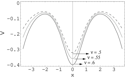
Figure 1: The potential, 2V is plotted as a function of x for different values of the parameter $\nu$, for $a_{1}$ = $0.009$ and $a_{2}$ = $\frac{\nu}{2}(\frac{\nu}{2}+1)$. The depth at $x=0$ increases with increasing $\nu$.

In this case one can obtain a double-barrier volcano potential with V(x) negative for all values of x. It is possible to have bound states at the location of the well. Assuming $a_{2}=\nu(\nu+1)$ we find a minimum at $x=0$ if $a_{2}>\nu a_{1}$. The profile depends on the parameter $\nu$ [Fig. (1)]. For the particle energies lesser than the depth of the potential well, there will be bound states. The potential decreases again beyond the turning points. Thus, there is a finite probability of tunneling through either barrier. This can be seen by assuming radiative boundary conditions at either infinity and calculating the tunneling probability in the same way as done for barrier penetration problems. As a result, there could be states found within the well which are quasibound. More precisely, these would be solutions with complex eigenvalues – the imaginary part being related to the lifetime of the quasibound state in the well. Some recent methods for the calculation of the lifetime of the quasibound states have been proposed in zamastil1 . We have plotted the potential for different values of the parameter $\nu$. It is apparent from Fig. (1) that the depth of the potential well increases with increasing values of the parameter $\nu$ ($a_{2}$). As a consequence, the probability of having a large number of bound states within the well gets more and more pronounced with increasing $\nu$.

Case II : ( $a_{1}=0$ and $a_{2}$ positive )

The potential obtained in this case is the well–known Pösch Teller potential (Fig. 2). The solutions of the Schrödinger equation reveals that the energy spectrum is continuous for the positive eigen values whereas it is discrete for negative eigenvalues of the energy lf . Discrete bound states are found inside the well.

Figure 2: The potential reduces to the well known Pösch-Teller potential for $a_{1}=0$ and $a_{2}$ positive.

Case III & IV : ( $a_{1}$, $a_{2}$ both negative / $a_{1}$ -ve, $a_{2}$ +ve )

For the single barrier potential (Case III) we essentially have the usual barrier penetration problem. In the last case, i.e. for a potential well, we can obtain bound states with a discrete energy spectrum. We intend to focus on the double-barrier volcano potential in the remaining part of this article.

Before we go over to solving the Schrodinger equation let us note the following fact. The volcano potential in the Case I above is not entirely unrelated to the inverted double well which we discussed at the beginning of this section. To see this, consider a Taylor expansion of the terms in the $cosh$–$sech$ volcano and retain terms up to order $x^{4}$. One will notice the reappearance of the $ax^{2}-bx^{4}$ potential for $\nu a_{1}<a_{2}$. Polynomial approximations for the other cases (II, III, IV) may also be obtained using the same expansion.

Exact solutions of the Schrödinger Equation: For the potential given in Eqn. (2), the Schrödinger equation is of the following form :

$$\frac{d^{2}\psi(x)}{dx^{2}}+(A_{1}\cosh^{2\nu}x+A_{2}\hskip 2.84544pt\mbox{sech}^{2}x+A_{3})\psi(x)=0$$ (3)

where, $A_{1}=2a_{1},A_{2}=2a_{2}$ and $A_{3}=2E$. It is possible to find an exact solution of the above equation if the relations, $A_{2}=\frac{\nu}{2}(\frac{\nu}{2}+1)$ and $A_{3}=-\frac{\nu^{2}}{4}$ are satisfied. The most general solution to Eqn. (3) is a combination of two linearly independent solutions, $\psi_{1}(x)$ and $\psi_{2}(x)$, given by

$$\psi_{1}(x)=A\frac{\cos\left[\sqrt{A_{1}}\hskip 2.84544pt\int(\cosh x)^{\nu}dx\right]}{(\cosh x)^{\frac{\nu}{2}}}$$ (4)

$$\psi_{2}(x)=B\frac{\sin\left[\sqrt{A_{1}}\hskip 2.84544pt\int(\cosh x)^{\nu}dx\right]}{(\cosh x)^{\frac{\nu}{2}}}$$ (5)

where, A and B are arbitrary constants, to be determined by the normalization condition. It is manifest from the general expressions that $\nu$ should be positive for the wave function to be finite at x $\rightarrow$ $\pm\infty$. The wave function is normalizable with $A=\left(\frac{\pi}{2}(1+e^{-2\sqrt{A_{1}}})\right)^{-\frac{1}{2}}$ and $B=\left(\frac{\pi}{2}(1-e^{-2\sqrt{A_{1}}})\right)^{-\frac{1}{2}}$ for $\nu=1$ with the normalization constant chosen as unity. The total energy of the particle is negative and the motion of the particle is bounded between the classical turning points of the potential when the particle’s energy lies between $V_{min}$ and the peak value of the potential i.e. $V_{min}<E<V_{max}$. The fact that the value of the bound state energy be within the well imposes a restriction of the allowed domain of $A_{1}$. This turns out to be $A_{1}>\frac{\nu}{2}$. Let us now explore how the states depend on different values of $\nu$. We show this graphically. The number of nodes of the wave function increases with increasing $\nu$ within a given region. In Fig. (3), we have plotted the wave functions for $\nu=1$ and $\nu=4$. The normalization constants are obtained for $\nu=1$ and one can argue that the wave functions are also normalizable for $\nu=4$ in the sense that ${|\psi|}^{2}$ covers a finite area for x $\rightarrow$ $\pm\infty$.

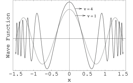
Figure 3: The even parity wave function, $\psi_{1}$(x) is plotted as a function of x for two different values of the parameter $\nu$ = 1 and 4. It is clear that the number of nodes increases with $\nu$ increasing.

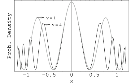
Figure 4: The probability density is plotted as a function of x for two different values of the parameter $\nu$ = 1 and 4 for even states. As both the curves are showing finite area we can conclude the wave functions are normalizable.

The probability density of the even states for the same set of $\nu$ values have been depicted in Fig. (4). From this we can conclude that the wave functions are normalizable and well behaved. The nature of the wave functions and probability density for the odd states with different values of the parameter $\nu$ are shown in Fig. (5) and (6) respectively.

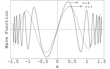
Figure 5: The odd parity wave function, $\psi_{2}$(x) is plotted as a function of x for two different values of the parameter $\nu=$ 1 and 4. It is clear that the number of nodes increases with $\nu$ increasing.

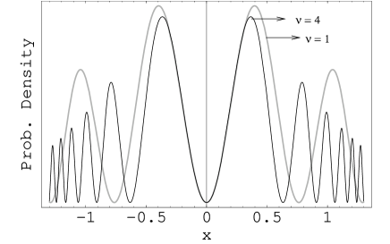
Figure 6: The probability density is plotted as a function of x for two different values of the parameter $\nu$ = 1 and 4 for odd states. As both the curves are showing finite area we can conclude the wave functions are normalizable.

The energy of the particle states can be calculated for definite values of $\nu$ from the relation, $A_{3}=-\frac{\nu^{2}}{4}$, which in turn implies that, $E_{\nu}=-\frac{\nu^{2}}{8}$. Energy eigenvalues are negative in this case. The even and odd parity states are degenerate though the model is one dimensional. This is an unusual feature which contradicts the usual theorems on definite parity bound states in symmetric potentials. We have not been able to obtain a better understanding of this curious feature of our solutions. However, the singularity in the potentials may provide the key to the understanding of degeneracy in one dimensions deg .

Furthermore, one can also evaluate the expectation values of $x$ and $p$ (using standard quantum mechanics) for these states. It turns out that:

$$\langle x\rangle=0\hskip 14.45377pt;\hskip 14.45377pt\langle p\rangle=0$$ (6)

However, one can check that $\langle x^{2}\rangle$ is finite, whereas $\langle p^{2}\rangle$ diverges to positive infinity. This implies that the uncertainty $\Delta x$ is finite, but the uncertainty $\Delta p$ is infinite. The curious fact is that, the kinetic energy  $T$ has a positively infinite expectation value, while $\langle V\rangle$ is negatively infinite but, $\langle H\rangle$ is finite. This happens because, in the integrand, the contributions from $T$ and $V$ which make their individual expectation values diverge, have opposite signs and therefore, cancel!

What can we say about a bound state which is infinitely spread out in position space? One notices that the even though the wave function is damped the number of nodes of the odd and even wave functions, within a small interval $dx$ increases with $x$. More specifically, we have

$$2n\pi=\sqrt{A_{1}}\int\left(\cosh x\right)^{\nu}dx$$

$$\frac{(2n+1)}{2}\pi=\sqrt{A_{1}}\int\left(\cosh x\right)^{\nu}dx$$ (7)

for the odd and even states, respectively. One can check easily that $\frac{dn}{dx}$ becomes progressively larger for large $x$ and fixed $dx$. This could be a reason for the divergence of the $\langle T\rangle$. In other words, the momentum space wavefunction has a significant contribution from the large momentum modes even though we have a localised bound state in position space parwani . It may be noted that there are positive energy bound states (in the continuum), the so–called von-Neumann–Wigner (vNW) states, which do have infinite number of nodes stillinger . However, apart from being positive energy states, note that for the vNW states, the potentials are bounded below unlike the potentials we have studied here. A better understanding of the peculiar bound states discussed in this article is surely desirable.

Concluding remarks : Let us now summarize our results. We have provided prescriptions for constructing volcano potentials which seem to have, of late, gained relevance in various areas of physics. After a brief discussion on classical mechanics in a volcano potential we have studied the quantum features in some detail. For a one–parameter family of such potentials we have been able to write down exact bound state solutions for specific values of the energy and the parameters in the potential. These solutions are normalizable in the usual sense (square integrable) though we find degenerate states of even and odd parity. We have shown through plots, the nature of the wave functions and probabilities for several cases. We have also calculated expectation values of position and momentum, the uncertainties in x and p and the density of nodes for our wavefunctions.

A point to note is that the potentials we have discussed lead to non-Hermitian Hamiltonians (due to the divergence to negative infinity of the potential). Though still a matter of debate, a fair amount of current work has shown some of the distinctive characteristics (eg. real eigenvalues for complex Hamiltonians. etc.) of such Hamiltonians (the so–called PT symmetric theory ptsymm ). The definition of observables as well as the construction of quantum mechanics needs modifications in the context of non–Hermiticity. Moreover, their physical utility remains an open question though we have mentioned some of them here. In fact, despite repeated use in high energy physics (braneworld models) the aspect of non–Hermiticity has never been mentioned in any article.

We hope the results derived in this paper may be useful in some way to researchers interested in pursuing the physics of volcano potentials.

SK thanks R. Parwani for discussions and some useful insights on various issues related to this article. RK thanks CSIR, India for financial support through a Senior Research Fellowship.

References

- (1) F. J. Gomez and L. Sesma, Phys. Letts. A301, 184 (2002); M. M. Nieto, Phys. Lett. B486,414 (2000); J.-Q. Liang and H. J. W. Muller–Kirsten, quant-ph/0407235
- (2) E Caliceti, V. Grecchi and M. Maioli, Commun. Math. Phys. 157,347 (1993); V. Buslaev and V. Grecchi, J. Phys. A: Math. Gen. 26, 5541 (1993)
- (3) L. L. Chang, L. Esaki, R. Tsu, Appl. Phys. Lett. 24, 593 (1974); Zhores. I. Alferov, Rev. Mod. Phys. 73(3), 767 (2001); J.C. Martinez and E. Polatdemir, quant-ph/0111103; B. Ricco and M. Ya. Azbel, Phys. Rev. B29, 1970 (1984); T.C. Au Yeung, Yabin Yu, W.Z. Shangguan and W.K. Chow, Phys. Rev. B68, 075316 (2003); W-C Tan and J. C. Inkson, Semicond. Sci. Technol. 11, 1635 (1996)
- (4) L. Randall and R. Sundrum, Phys. Rev. Lett. 83, 4690 (1999); C. Csaki, J. Erlich, T. J. Hollowood, and Y. Shirman, Nucl. Phys. B581, 309 (2000); R. Koley and S. Kar, Class. Quant. Grav. 22, 753 (2005); N. Barbosa-Cendejas and A. Herrera-Aguilar, Phys. Rev D73, 084022 (2006)
- (5) J. Zamastil, J. Cizek and L. Skala, Phys. Rev. Letts. 84, 5683 (2000); J. Zamastil, V. Spirko, J. Cizek, L. Skala and O. Bludsky, Phys. Rev. A 64, 042101 (2001)
- (6) C. Bender, Introduction to PT symmetric quantum theory, quant-ph/0501052
- (7) I. Percival and D. Richards, Introduction to Dynamics, Pg 2-3 (Cambridge University Press, 1982)
- (8) L.D. Landau and E.M. Lifshitz, Quantum Mechanics, Course of Theoretical Physics, Vol. 3, Third Edition (Butterworth - Heinemann, 1977).
- (9) K. Bhattacharyya and R. K. Pathak, Int. J. Quantum Chem. 59, 219 (1996)
- (10) R. Parwani, private communication
- (11) F. H. Stillinger and D. R. Herrick, Phys. Rev. A 11, 446 (1975)