A Straightforward Introduction to Continuous Quantum Measurement

Abstract

We present a pedagogical treatment of the formalism of continuous quantum measurement. Our aim is to show the reader how the equations describing such measurements are derived and manipulated in a direct manner. We also give elementary background material for those new to measurement theory, and describe further various aspects of continuous measurements that should be helpful to those wanting to use such measurements in applications. Specifically, we use the simple and direct approach of generalized measurements to derive the stochastic master equation describing the continuous measurements of observables, give a tutorial on stochastic calculus, treat multiple observers and inefficient detection, examine a general form of the measurement master equation, and show how the master equation leads to information gain and disturbance. To conclude, we give a detailed treatment of imaging the resonance fluorescence from a single atom as a concrete example of how a continuous position measurement arises in a physical system.

I Introduction

When measurement is first introduced to students of quantum mechanics, it is invariably treated by ignoring any consideration of the time the measurement takes: the measurement just “happens,” for all intents and purposes, instantaneously. This treatment is good for a first introduction, but is not sufficient to describe two important situations. The first is when some aspect of a system is continually monitored. This happens, for example, when one illuminates an object and continually detects the reflected light in order to track the object’s motion. In this case, information is obtained about the object at a finite rate, and one needs to understand what happens to the object while the measurement takes place. It is the subject of continuous quantum measurement that describes such a measurement. The second situation arises because nothing really happens instantaneously. Even rapid, “single shot” measurements take some time. If this time is not short compared to the dynamics of the measured system, then it is once again important to understand both the dynamics of the flow of information to the observer and the effect of the measurement on the system.

Continuous measurement has become increasingly important in the last decade, due mainly to the growing interest in the application of feedback control in quantum systems Belavkin (1987); Doherty and Jacobs (1999); Wiseman and Doherty (2005); Hopkins et al. (2003); Steck et al. (2004); Steixner et al. (2005); Rabl et al. (2005); Combes and Jacobs (2006); Bushev et al. (2006); D’Helon and James (2006); Steck et al. (2006). In feedback control a system is continuously measured, and this information is used while the measurement proceeds (that is, in real time) to modify the system Hamiltonian so as to obtain some desired behavior. Thus, continuous measurement theory is essential for describing feedback control. The increasing interest in continuous measurement is also due to its applications in metrology Wiseman (1995); Berry and Wiseman (2002); Pope et al. (2004); Stockton et al. (2004); Geremia et al. (2005), quantum information Dolinar (1973); Geremia (2004); Jacobs (2007), quantum computing Ahn et al. (2002); Sarovar et al. (2004); van Handel and Mabuchi (2006), and its importance in understanding the quantum to classical transition Bhattacharya et al. (2000); Habib et al. (2002); Bhattacharya et al. (2003); Ghose et al. (2004, 2005); Everitt et al. (2005); Habib et al. (2006).

While the importance of continuous measurement grows, to date there is really only one introduction to the subject that could be described as both easily accessible and extensive, that being the one by Brun in the American Journal of Physics Brun (2002) (some other pedagogical treatments can be found in Braginsky et al. (1995); Carmichael (1993); Wiseman (1996a)). While the analysis in Brun’s work is suitably direct, it treats explicitly only measurements on two-state systems, and due to their simplicity the derivations used there do not easily extend to measurements of more general observables. Since many applications involve measurements of observables in infinite-dimensional systems (such as the position of a particle), we felt that an introductory article that derived the equations for such measurements in the simplest and most direct fashion would fill an important gap in the literature. This is what we do here. Don’t be put off by the length of this article—a reading of only a fraction of the article is sufficient to understand how to derive the basic equation that describes continuous measurement, the mathematics required to manipulate it (the so-called Itô calculus), and how it can be solved. This is achieved in Sections IV, V, and VI. If the reader is not familiar with the density operator, then this preliminary material is explained in Section II, and generalized quantum measurements (POVM’s) are explained in Section III.

The rest of the article gives some more information about continuous measurements. In Section VII we show how to treat multiple, simultaneous observers and inefficient detectors, both of which involve simple and quite straightforward generalizations of the basic equation. In Section VIII we discuss the most general form that the continuous-measurement equation can take. In Section IX we present explicit calculations to explain the meaning of the various terms in the measurement equation. Since our goal in the first part of this article was to derive a continuous measurement equation in the shortest and most direct manner, this did not involve a concrete physical example. In the second-to-last (and longest) section, we provide such an example, showing in considerable detail how a continuous measurement arises when the position of an atom is monitored by detecting the photons it emits. The final section concludes with some pointers for further reading.

II Describing an Observer’s State of Knowledge of a Quantum System

II.1 The Density Operator

Before getting on with measurements, we will briefly review the density operator, since it is so central to our discussion. The density operator represents the state of a quantum system in a more general way than the state vector, and equivalently represents an observer’s state of knowledge of a system.

When a quantum state can be represented by a state vector $|{\psi}\rangle$, the density operator is defined as the product

$$\rho:=|{\psi}\rangle\langle{\psi}|.$$ (1)

In this case, it is obvious that the information content of the density operator is equivalent to that of the state vector (except for the overall phase, which is not of physical significance).

The state vector can represent states of coherent superposition. The power of the density operator lies in the fact that it can represent incoherent superpositions as well. For example, let $|{\psi_{\alpha}}\rangle$ be a set of states (without any particular restrictions). Then the density operator

$$\rho=\sum_{\alpha}p_{\alpha}|{\psi_{\alpha}}\rangle\langle{\psi_{\alpha}}|$$ (2)

models the fact that we don’t know which of the states $|{\psi_{\alpha}}\rangle$ the system is in, but we know that it is in the state $|{\psi_{\alpha}}\rangle$ with probability $p_{\alpha}$. Another way to say it is this: the state vector $|{\psi}\rangle$ represents a certain intrinsic uncertainty with respect to quantum observables; the density operator can represent uncertainty beyond the minimum required by quantum mechanics. Equivalently, the density operator can represent an ensemble of identical systems in possibly different states.

A state of the form $(\ref{rhopure})$ is said to be a pure state. One that cannot be written in this form is said to be mixed, and can be written in the form (2).

Differentiating the density operator and employing the Schrödinger equation $i\hbar\partial_{t}|{\psi}\rangle=H|{\psi}\rangle$, we can write down the equation of motion for the density operator:

$$\partial_{t}\rho=-\,\frac{i}{\hbar}[H,\rho].$$ (3)

This is referred to as the Schrödinger–von Neumann equation. Of course, the use of the density operator allows us to write down more general evolution equations than those implied by state-vector dynamics.

II.2 Expectation Values

We can compute expectation values with respect to the density operator via the trace operation. The trace of an operator $A$ is simply the sum over the diagonal matrix elements with respect to any complete, orthonormal set of states $|{\beta}\rangle$:

$$\mathrm{Tr}[A]:=\sum_{\beta}\langle{\beta}|A|{\beta}\rangle.$$ (4)

An important property of the trace is that the trace of a product is invariant under cyclic permutations of the product. For example, for three operators,

$$\mathrm{Tr}[ABC]=\mathrm{Tr}[BCA]=\mathrm{Tr}[CAB].$$ (5)

This amounts to simply an interchange in the order of summations. For example, for two operators, working in the position representation, we can use the fact that $\int dx\,\langle x|{x}\rangle$ is the identity operator to see that

$$\begin{array}[]{rcl}\mathrm{Tr}[AB]&{}={}&\displaystyle\int dx\langle{x}|AB|{x}\rangle\\ &{}={}&\displaystyle\int dx\int dx^{\prime}\,\langle{x}|A|{x^{\prime}}\rangle\langle{x^{\prime}}|B|{x}\rangle\\ &{}={}&\displaystyle\int dx^{\prime}\int dx\,\langle{x^{\prime}}|B|{x}\rangle\langle{x}|A|{x^{\prime}}\rangle\\ &{}={}&\displaystyle\int dx^{\prime}\langle{x^{\prime}}|BA|{x^{\prime}}\rangle\\ &{}={}&\displaystyle\mathrm{Tr}[BA].\end{array}$$ (6)

Note that this argument assumes sufficiently “nice” operators (it fails, for example, for $\mathrm{Tr}[xp]$). More general permutations [e.g., of the form (5)] are obtained by replacements of the form $B\longrightarrow BC$. Using this property, we can write the expectation value with respect to a pure state as

$$\!\left\langle{A}\right\rangle=\!\left\langle{\psi|A|\psi}\right\rangle=\mathrm{Tr}[A\rho].$$ (7)

This argument extends to the more general form (2) of the density operator.

II.3 The Density Matrix

The physical content of the density matrix is more apparent when we compute the elements $\rho_{\alpha\alpha^{\prime}}$ of the density matrix with respect to a complete, orthonormal basis. The density matrix elements are given by

$$\rho_{\alpha\alpha^{\prime}}:=\langle{\alpha}|\rho|{\alpha^{\prime}}\rangle.$$ (8)

To analyze these matrix elements, we will assume the simple form $\rho=|{\psi}\rangle\langle{\psi}|$ of the density operator, though the arguments generalize easily to arbitrary density operators.

The diagonal elements $\rho_{\alpha\alpha}$ are referred to as populations, and give the probability of being in the state $|{\alpha}\rangle$:

$$\rho_{\alpha\alpha}=\langle{\alpha}|\rho|{\alpha}\rangle=\left|\!\left\langle{\alpha|\psi}\right\rangle\right|^{2}.$$ (9)

The off-diagonal elements $\rho_{\alpha\alpha^{\prime}}$ (with $\alpha\neq\alpha^{\prime}$) are referred to as coherences, since they give information about the relative phase of different components of the superposition. For example, if we write the state vector as a superposition with explicit phases,

$$|{\psi}\rangle=\sum_{\alpha}c_{\alpha}|{\alpha}\rangle=\sum_{\alpha}|c_{\alpha}|e^{i\phi_{\alpha}}|{\alpha}\rangle,$$ (10)

then the coherences are

$$\rho_{\alpha\alpha^{\prime}}=|c_{\alpha}c_{\alpha^{\prime}}|e^{i(\phi_{\alpha}-\phi_{\alpha^{\prime}})}.$$ (11)

Notice that for a density operator not corresponding to a pure state, the coherences in general will be the sum of complex numbers corresponding to different states in the incoherent sum. The phases will not in general line up, so that while $|\rho_{\alpha\alpha^{\prime}}|^{2}=\rho_{\alpha\alpha}\rho_{\alpha^{\prime}\alpha^{\prime}}$ for a pure state, we expect $|\rho_{\alpha\alpha^{\prime}}|^{2}<\rho_{\alpha\alpha}\rho_{\alpha^{\prime}\alpha^{\prime}}$ ($\alpha\neq\alpha^{\prime}$) for a generic mixed state.

II.4 Purity

The difference between pure and mixed states can be formalized in another way. Notice that the diagonal elements of the density matrix form a probability distribution. Proper normalization thus requires

$$\mathrm{Tr}[\rho]=\sum_{\alpha}\rho_{\alpha\alpha}=1.$$ (12)

We can do the same computation for $\rho^{2}$, and we will define the purity to be $\mathrm{Tr}[\rho^{2}]$. For a pure state, the purity is simple to calculate:

$$\mathrm{Tr}[\rho^{2}]=\mathrm{Tr}[|{\psi}\rangle\langle\psi|\psi\rangle\langle{\psi}|]=\mathrm{Tr}[\rho]=1.$$ (13)

But for mixed states, $\mathrm{Tr}[\rho^{2}]<1$. For example, for the density operator in (2),

$$\mathrm{Tr}[\rho^{2}]=\sum_{\alpha}p_{\alpha}^{\,2},$$ (14)

if we assume the states $|{\psi_{\alpha}}\rangle$ to be orthonormal. For equal probability of being in $N$ such states, $\mathrm{Tr}[\rho^{2}]=1/N$. Intuitively, then, we can see that $\mathrm{Tr}[\rho^{2}]$ drops to zero as the state becomes more mixed—that is, as it becomes an incoherent superposition of more and more orthogonal states.

III Weak Measurements and POVM’s

In undergraduate courses the only kind of measurement that is usually discussed is one in which the system is projected onto one of the possible eigenstates of a given observable. If we write these eigenstates as $\{|n\rangle:n=1,\ldots,n_{\mathrm{max}}\}$, and the state of the system is $|\psi\rangle=\sum_{n}c_{n}|n\rangle$, the probability that the system is projected onto $|n\rangle$ is $|c_{n}|^{2}$. In fact, these kind of measurements, which are often referred to as von Neumann measurements, represent only a special class of all the possible measurements that can be made on quantum systems. However, all measurements can be derived from von Neumann measurements.

One reason that we need to consider a larger class of measurements is so we can describe measurements that extract only partial information about an observable. A von Neumann measurement provides complete information—after the measurement is performed we know exactly what the value of the observable is, since the system is projected into an eigenstate. Naturally, however, there exist many measurements which, while reducing on average our uncertainty regarding the observable of interest, do not remove it completely.

First, it is worth noting that a von Neumann measurement can be described by using a set of projection operators $\{P_{n}=|n\rangle\langle n|\}$. Each of these operators describes what happens on one of the possible outcomes of the measurement: if the initial state of the system is $\rho=|\psi\rangle\langle\psi|$, then the $n$th possible outcome of the final state is given by

$$\rho_{\mathrm{f}}=|n\rangle\langle n|=\frac{P_{n}\rho P_{n}}{\mathrm{Tr}[P_{n}\rho P_{n}]},$$ (15)

and this result is obtained with probability

$$P(n)=\mbox{Tr}[P_{n}\rho P_{n}]=c_{n},$$ (16)

where $c_{n}$ defines the superposition of the initial state $|{\psi}\rangle$ given above. It turns out that every possible measurement may be described in a similar fashion by generalizing the set of operators. Suppose we pick a set of $m_{\mathrm{max}}$ operators $\Omega_{m}$, the only restriction being that $\sum_{m=1}^{m_{\mathrm{max}}}\Omega_{m}^{\dagger}\Omega_{m}=I$, where $I$ is the identity operator. Then it is in principle possible to design a measurement that has $N$ possible outcomes,

$$\rho_{\mathrm{f}}=\frac{\Omega_{m}\rho\Omega_{m}^{\dagger}}{\mathrm{Tr}[\Omega_{m}\rho\Omega_{m}^{\dagger}]},$$ (17)

with

$$P(m)=\mathrm{Tr}[\Omega_{m}\rho\Omega_{m}^{\dagger}]$$ (18)

giving the probability of obtaining the $m$th outcome.

Every one of these more general measurements may be implemented by performing a unitary interaction between the system and an auxiliary system, and then performing a von Neumann measurement on the auxiliary system. Thus all possible measurements may be derived from the basic postulates of unitary evolution and von Neumann measurement Schumacher (1996); Nielsen and Chuang (2000).

These “generalized” measurements are often referred to as POVM’s, where the acronym stands for “positive operator-valued measure.” The reason for this is somewhat technical, but we explain it here because the terminology is so common. Note that the probability for obtaining a result in the range $[a,b]$ is

$$P(m\in[a,b])=\sum_{m=a}^{b}\mbox{Tr}\left[\Omega_{m}\rho\Omega_{m}^{\dagger}\right]=\mbox{Tr}\left[\sum_{m=a}^{b}\Omega_{m}^{\dagger}\Omega_{m}\rho\right].$$ (19)

The positive operator $M=\sum_{m=a}^{b}\Omega_{m}^{\dagger}\Omega_{m}$ thus determines the probability that $m$ lies in the subset $[a,b]$ of its range. In this way the formalism associates a positive operator with every subset of the range of $m$, and is therefore a positive operator-valued measure.

Let us now put this into practice to describe a measurement that provides partial information about an observable. In this case, instead of our measurement operators $\Omega_{m}$ being projectors onto a single eigenstate, we choose them to be a weighted sum of projectors onto the eigenstates $|n\rangle$, each one peaked about a different value of the observable. Let us assume now, for the sake of simplicity, that the eigenvalues $n$ of the observable $N$ take on all the integer values. In this case we can choose

$$\Omega_{m}=\frac{1}{\cal N}\sum_{n}e^{-k(n-m)^{2}/4}|n\rangle\langle n|,$$ (20)

where ${\cal N}$ is a normalization constant chosen so that $\sum_{m=-\infty}^{\infty}\Omega_{m}^{\dagger}\Omega_{m}=I$. We have now constructed a measurement that provides partial information about the observable $N$. This is illustrated clearly by examining the case where we start with no information about the system. In this case the density matrix is completely mixed, so that $\rho\propto I$. After making the measurement and obtaining the result $m$, the state of the system is

$$\rho_{\mbox{\scriptsize f}}=\frac{\Omega_{m}\rho\Omega_{m}^{\dagger}}{\mbox{Tr}[\Omega_{m}\rho\Omega_{m}^{\dagger}]}=\frac{1}{\cal N}\sum_{n}e^{-k(n-m)^{2}/2}|n\rangle\langle n|.$$ (21)

The final state is thus peaked about the eigenvalue $m$, but has a width given by $1/\sqrt{k}$. The larger $k$, the less our final uncertainty regarding the value of the observable. Measurements for which $k$ is large are often referred to as strong measurements, and conversely those for which $k$ is small are weak measurements Fuchs and Jacobs (2001). These are the kinds of measurements that we will need in order to derive a continuous measurement in the next section.

IV A Continuous Measurement of an Observable

A continuous measurement is one in which information is continually extracted from a system. Another way to say this is that when one is making such a measurement, the amount of information obtained goes to zero as the duration of the measurement goes to zero. To construct a measurement like this, we can divide time into a sequence of intervals of length $\Delta t$, and consider a weak measurement in each interval. To obtain a continuous measurement, we make the strength of each measurement proportional to the time interval, and then take the limit in which the time intervals become infinitesimally short.

In what follows, we will denote the observable we are measuring by $X$ (i.e., $X$ is a Hermitian operator), and we will assume that it has a continuous spectrum of eigenvalues $x$. We will write the eigenstates as $|x\rangle$, so that $\langle x|x^{\prime}\rangle=\delta(x-x^{\prime})$. However, the equation that we will derive will be valid for measurements of any Hermitian operator.

We now divide time into intervals of length $\Delta t$. In each time interval, we will make a measurement described by the operators

$$A(\alpha)=\left(\frac{4k\Delta t}{\pi}\right)^{1/4}\int_{-\infty}^{\infty}e^{-2k\Delta t(x-\alpha)^{2}}|x\rangle\langle x|dx.$$ (22)

Each operator $A(\alpha)$ a Gaussian-weighted sum of projectors onto the eigenstates of $X$. Here $\alpha$ is a continuous index, so that there is a continuum of measurement results labeled by $\alpha$.

The first thing we need to know is the probability density $P(\alpha)$ of the measurement result $\alpha$ when $\Delta t$ is small. To work this out we first calculate the mean value of $\alpha$. If the initial state is $|\psi\rangle=\int\psi(x)|x\rangle dx$ then $P(\alpha)=\mbox{Tr}[A(\alpha)^{\dagger}A(\alpha)|\psi\rangle\langle\psi|]$, and we have

$$\begin{array}[]{rcl}\langle\alpha\rangle&{}={}&\displaystyle\int_{-\infty}^{\infty}\alpha P(\alpha)\,d\alpha\\ &{}={}&\displaystyle\int_{-\infty}^{\infty}\alpha\mbox{Tr}[A(\alpha)^{\dagger}A(\alpha)|\psi\rangle\langle\psi|]\,d\alpha\\ &{}={}&\displaystyle\sqrt{\frac{4k\Delta t}{\pi}}\int_{-\infty}^{\infty}\int_{-\infty}^{\infty}\alpha|\psi(x)|^{2}e^{-4k\Delta t(x-\alpha)^{2}}\,dx\,d\alpha\\ &{}={}&\displaystyle\int_{-\infty}^{\infty}x|\psi(x)|^{2}\,dx=\langle X\rangle.\end{array}$$ (23)

To obtain $P(\alpha)$ we now write

$$\begin{array}[]{rcl}P(\alpha)&{}={}&\displaystyle\mbox{Tr}[A(\alpha)^{\dagger}A(\alpha)|\psi\rangle\langle\psi|]\\ &{}={}&\displaystyle\sqrt{\frac{4k\Delta t}{\pi}}\int_{-\infty}^{\infty}|\psi(x)|^{2}e^{-4k\Delta t(x-\alpha)^{2}}dx.\end{array}$$ (24)

If $\Delta t$ is sufficiently small then the Gaussian is much broader than $\psi(x)$. This means we can approximate $|\psi(x)|^{2}$ by a delta function, which must be centered at the expected position $\langle X\rangle$ so that $\langle\alpha\rangle=\langle X\rangle$ as calculated above. We therefore have

$$\begin{array}[]{rcl}P(\alpha)&{}\approx{}&\displaystyle\sqrt{\frac{4k\Delta t}{\pi}}\int_{-\infty}^{\infty}\delta(x-\!\left\langle{X}\right\rangle)e^{-4k\Delta t(x-\alpha)^{2}}\;dx\\ &{}={}&\displaystyle\sqrt{\frac{4k\Delta t}{\pi}}e^{-4k\Delta t(\alpha-\langle X\rangle)^{2}}.\end{array}$$ (25)

We can also write $\alpha$ as the stochastic quantity

$$\alpha_{\mathrm{s}}=\langle X\rangle+\frac{\Delta W}{\sqrt{8k}\Delta t},$$ (26)

where $\Delta W$ is a zero-mean, Gaussian random variable with variance $\Delta t$. This alternate representation as a stochastic variable will be useful later. Since it will be clear from context, we will use $\alpha$ interchangeably with $\alpha_{\mathrm{s}}$ in referring to the measurement results, although technically we should distinguish between the index $\alpha$ and the stochastic variable $\alpha_{\mathrm{s}}$.

A continuous measurement results if we make a sequence of these measurements and take the limit as $\Delta t\longrightarrow 0$ (or equivalently, as $\Delta t\longrightarrow dt$). As this limit is taken, more and more measurements are made in any finite time interval, but each is increasingly weak. By choosing the variance of the measurement result to scale as $\Delta t$, we have ensured that we obtain a sensible continuum limit. A stochastic equation of motion results due to the random nature of the measurements (a stochastic variable is one that fluctuates randomly over time). We can derive this equation of motion for the system under this continuous measurement by calculating the change induced in the quantum state by the single weak measurement in the time step $\Delta t$, to first order in $\Delta t$. We will thus compute the evolution when a measurement, represented by the operator $A(\alpha)$, is performed in each time step. This procedure gives

$$\begin{array}[]{rcl}|\psi(t+\Delta t)\rangle&{}\propto{}&\displaystyle A(\alpha)|\psi(t)\rangle\\ &{}\propto{}&\displaystyle e^{-2k\Delta t(\alpha-X)^{2}}|\psi(t)\rangle\\ &{}\propto{}&\displaystyle e^{-2k\Delta tX^{2}+X[4k\langle X\rangle\Delta t+\sqrt{2k}\Delta W]}|\psi(t)\rangle.\end{array}$$ (27)

We now expand the exponential to first order in $\Delta t$, which gives

$$|\psi(t+\Delta t)\rangle\propto\{1-2k\Delta tX^{2}+X[4k\langle X\rangle\Delta t+\sqrt{2k}\Delta W+kX(\Delta W)^{2}]\}|\psi(t)\rangle.$$ (28)

Note that we have included the second-order term in $\Delta W$ in the power series expansion for the exponential. We need to include this term because it turns out that in the limit in which $\Delta t\longrightarrow 0$, $(\Delta W)^{2}\longrightarrow(dW)^{2}=dt$. Because of this, the $(\Delta W)^{2}$ term contributes to the final differential equation. The reason for this will be explained in the next section, but for now we ask the reader to indulge us and accept that it is true.

To take the limit as $\Delta t\rightarrow 0$, we set $\Delta t=dt$, $\Delta W=dW$ and $(\Delta W)^{2}=dt$, and the result is

$$|\psi(t+dt)\rangle\propto\{1-[kX^{2}-4kX\langle X\rangle]\,dt+\sqrt{2k}X\,dW\}|\psi(t)\rangle.$$ (29)

This equation does not preserve the norm $\langle\psi|\psi\rangle$ of the wave function, because before we derived it we threw away the normalization. We can easily obtain an equation that does preserve the norm simply by normalizing $|\psi(t+dt)\rangle$ and expanding the result to first order in $dt$ (again, keeping terms to order $dW^{2}$). Writing $|\psi(t+dt)\rangle=|\psi(t)\rangle+d|\psi\rangle$, the resulting stochastic differential equation is given by

$$d|\psi\rangle=\{-k(X-\langle X\rangle)^{2}dt+\sqrt{2k}(X-\langle X\rangle)\,dW\}|\psi(t)\rangle.$$ (30)

This is the equation we have been seeking—it describes the evolution of the state of a system in a time interval $dt$ given that the observer obtains the measurement result

$$dy=\langle X\rangle\,dt+\frac{dW}{\sqrt{8k}}$$ (31)

in that time interval. The measurement result gives the expected value $\,\!\left\langle{X}\right\rangle$ plus a random component due to the width of $P(\alpha)$, and we write this as a differential since it corresponds to the information gained in the time interval $dt$. As the observer integrates $dy(t)$ the quantum state progressively collapses, and this integration is equivalent to solving (30) for the quantum-state evolution.

The stochastic Schrödinger equation (SSE) in Eq. (30) is usually described as giving the evolution conditioned upon the stream of measurement results. The state $|{\psi}\rangle$ evolves randomly, and $|{\psi(t)}\rangle$ is called the quantum trajectory Carmichael (1993). The set of measurement results $dy(t)$ is called the measurement record. We can also write this SSE in terms of the density operator $\rho$ instead of $|\psi\rangle$. Remembering that we must keep all terms proportional to $dW^{2}$, and defining $\rho(t+dt)\equiv\rho(t)+d\rho$, we have

$$\begin{array}[]{rcl}d\rho&{}={}&\displaystyle(d|\psi\rangle)\langle\psi|+|\psi\rangle(d\langle\psi|)+(d|\psi\rangle)(d\langle\psi|)\\ &{}={}&\displaystyle-k[X[X,\rho]]\,dt\\ &&\displaystyle{}+\sqrt{2k}(X\rho+\rho X-2\langle X\rangle\rho)dW.\end{array}$$ (32)

This is referred to as a stochastic master equation (SME), which also defines a quantum trajectory $\rho(t)$. This SME was first derived by Belavkin Belavkin (1987). Note that in general, the SME also includes a term describing Hamiltonian evolution as in Eq. (3).

The density operator at time $t$ gives the observer’s state of knowledge of the system, given that she has obtained the measurement record $y(t)$ up until time $t$. Since the observer has access to $dy$ but not to $dW$, to calculate $\rho(t)$ she must calculate $dW$ at each time step from the measurement record in that time step along with the expectation value of $X$ at the previous time:

$$dW=\sqrt{8k}\,(dy-\langle X\rangle\,dt).$$ (33)

By substituting this expression in the SME [Eq. (32)], we can write the evolution of the system directly in terms of the measurement record, which is the natural thing to do from the point of the view of the observer. This is

$$\begin{array}[]{rcl}d\rho&{}={}&\displaystyle-k[X[X,\rho]]\,dt\\ &&\displaystyle{}+4k(X\rho+\rho X-2\langle X\rangle\rho)(dy-\langle X\rangle\,dt).\end{array}$$ (34)

In Section VI we will explain how to solve the SME analytically in a special case, but it is often necessary to solve it numerically. The simplest method of doing this is to take small time steps $\Delta t$, and use a random number generator to select a new $\Delta W$ in each time step. One then uses $\Delta t$ and $\Delta W$ in each time step to calculate $\Delta\rho$ and adds this to the current state $\rho$. In this way we generate a specific trajectory for the system. Each possible sequence of $dW$’s generates a different trajectory, and the probability that a given trajectory occurs is the probability that the random number generator gives the corresponding sequence of $dW$’s. A given sequence of $dW$’s is often referred to as a “realization” of the noise, and we will refer to the process of generating a sequence of $dW$’s as “picking a noise realization”. Further details regarding the numerical methods for solving stochastic equations are given in Kloeden and Platen (1992).

If the observer makes the continuous measurement, but throws away the information regarding the measurement results, the observer must average over the different possible results. Since $\rho$ and $dW$ are statistically independent, $\left\langle\!\left\langle{\rho\,dW}\right\rangle\!\right\rangle=0$, where the double brackets denote this average (as we show in Section V.2.3). The result is thus given by setting to zero all terms proportional to $\rho\,dW$ in Eq. (32),

$$\frac{d\rho}{dt}=-k[X[X,\rho]],$$ (35)

where the density operator here represents the state averaged over all possible measurement results. We note that the method we have used above to derive the stochastic Schrödinger equation is an extension of a method initially developed by Caves and Milburn to derive the (non-stochastic) master equation (35) Caves and Milburn (1987).

V An Introduction to Stochastic Calculus

Now that we have encountered a noise process in the quantum evolution, we will explore in more detail the formalism for handling this. It turns out that adding a white-noise stochastic process changes the basic structure of the calculus for treating the evolution equations. There is more than one formulation to treat stochastic processes, but the one referred to as Itô calculus is used in almost all treatments of noisy quantum systems, and so this is the one we describe here. The main alternative formalism may be found in Refs. Gardiner (1985); Kloeden and Platen (1992).

V.1 Usage

First, let’s review the usual calculus in a slightly different way. A differential equation

$$\frac{dy}{dt}=\alpha$$ (36)

can be instead written in terms of differentials as

$$dy=\alpha\,dt.$$ (37)

The basic rule in the familiar deterministic calculus is that $(dt)^{2}=0$. To see what we mean by this, we can try calculating the differential $dz$ for the variable $z=e^{y}$ in terms of the differential for $dy$ as follows:

$$dz=e^{y+dy}-e^{y}=z\left(e^{\alpha\,dt}-1\right).$$ (38)

Expanding the exponential and applying the rule $(dt)^{2}=0$, we find

$$dz=z\alpha\,dt.$$ (39)

This is, of course, the same result as that obtained by using the chain rule to calculate $dz/dy$ and multiplying through by $dy$. The point here is that calculus breaks up functions and considers their values within short intervals $\Delta t$. In the infinitesimal limit, the quadratic and higher order terms in $\Delta t$ end up being too small to contribute.

In Itô calculus, we have an additional differential element $dW$, representing white noise. The basic rule of Itô calculus is that $dW^{2}=dt$, while $dt^{2}=dt\,dW=0$. We will justify this later, but to use this calculus, we simply note that we “count” the increment $dW$ as if it were equivalent to $\sqrt{dt}$ in deciding what orders to keep in series expansions of functions of $dt$ and $dW$. As an example, consider the stochastic differential equation

$$dy=\alpha\,dt+\beta\,dW.$$ (40)

We obtain the corresponding differential equation for $z=e^{y}$ by expanding to second order in $dy$:

$$dz=e^{y}\left(e^{dy}-1\right)=z\left(dy+\frac{(dy)^{2}}{2}\right).$$ (41)

Only the $dW$ component contributes to the quadratic term; the result is

$$dz=z\left(\alpha+\frac{\beta^{2}}{2}\right)\,dt+z\beta\,dW.$$ (42)

The extra $\beta^{2}$ term is crucial in understanding many phenomena that arise in continuous-measurement processes.

V.2 Justification

V.2.1 Wiener Process

To see why all this works, let’s first define the Wiener process $W(t)$ as an “ideal” random walk with arbitrarily small, independent steps taken arbitrarily often. (The Wiener process is thus scale-free and in fact fractal.) Being a symmetric random walk, $W(t)$ is a normally distributed random variable with zero mean, and we choose the variance of $W(t)$ to be $t$ (i.e., the width of the distribution is $\sqrt{t}$, as is characteristic of a diffusive process). We can thus write the probability density for $W(t)$ as

$$P(W,t)=\frac{1}{\sqrt{2\pi t}}e^{-W^{2}/2t}.$$ (43)

In view of the central-limit theorem, any simple random walk gives rise to a Wiener process in the continuous limit, independent of the one-step probability distribution (so long as the one-step variance is finite).

Intuitively, $W(t)$ is a continuous but everywhere nondifferentiable function. Naturally, the first thing we will want to do is to develop the analogue of the derivative for the Wiener process. We can start by defining the Wiener increment

$$\Delta W(t):=W(t+\Delta t)-W(t)$$ (44)

corresponding to a time increment $\Delta t$. Again, $\Delta W$ is a normally distributed random variable with zero mean and variance $\Delta t$. Note again that this implies that the root-mean-square amplitude of $\Delta W$ scales as $\sqrt{\Delta t}$. We can understand this intuitively since the variances add for successive steps in a random walk. Mathematically, we can write the variance as

$$\left\langle\!\left\langle{(\Delta W)^{2}}\right\rangle\!\right\rangle=\Delta t,$$ (45)

where the double angle brackets $\left\langle\!\left\langle{~{}}\right\rangle\!\right\rangle$ denote an ensemble average over all possible realizations of the Wiener process. This relation suggests the above notion that second-order terms in $\Delta W$ contribute at the same level as first-order terms in $\Delta t$. In the infinitesimal limit of $\Delta t\longrightarrow 0$, we write $\Delta t\longrightarrow dt$ and $\Delta W\longrightarrow dW$.

V.2.2 Itô Rule

We now want to show that the Wiener differential $dW$ satisfies the Itô rule $dW^{2}=dt$. Note that we want this to hold without the ensemble average, which is surprising since $dW$ is a stochastic quantity, while $dt$ obviously is not. To do this, consider the probability density function for $(\Delta W)^{2}$, which we can obtain by a simple transformation of the Gaussian probability density for $\Delta W$ [which is Eq. (43) with $t\longrightarrow\Delta t$ and $W\longrightarrow\Delta W$]:

$$P\left[(\Delta W)^{2}\right]=\frac{e^{-(\Delta W)^{2}/2\Delta t}}{\sqrt{2\pi\,\Delta t\,(\Delta W)^{2}}}.$$ (46)

In particular, the mean and variance of this distribution for $(\Delta W)^{2}$ are

$$\left\langle\!\left\langle{(\Delta W)^{2}}\right\rangle\!\right\rangle=\Delta t$$ (47)

and

$$\textrm{Var}\left[(\Delta W)^{2}\right]=2(\Delta t)^{2},$$ (48)

respectively. To examine the continuum limit, we will sum the Wiener increments over $N$ intervals of duration $\Delta t_{N}=t/N$ between $0$ and $t$. The corresponding Wiener increments are

$$\Delta W_{n}:=W[(n+1)\Delta t_{N}]-W(n\Delta t_{N}).$$ (49)

Now consider the sum of the squared increments

$$\sum_{n=0}^{N-1}(\Delta W_{n})^{2},$$ (50)

which corresponds to a random walk of $N$ steps, where a single step has average value $t/N$ and variance $2t^{2}/N^{2}$. According to the central limit theorem, for large $N$ the sum (50) is a Gaussian random variable with mean $t$ and variance $2t^{2}/N$. In the limit $N\longrightarrow\infty$, the variance of the sum vanishes, and the sum becomes $t$ with certainty. Symbolically, we can write

$$\int_{0}^{t}[dW(t^{\prime})]^{2}:=\lim_{N\rightarrow\infty}\sum_{n=0}^{N-1}(\Delta W_{n})^{2}=t=\int_{0}^{t}dt^{\prime}.$$ (51)

For this to hold over any interval $(0,t)$, we must make the formal identification $dt=dW^{2}$. This means that even though $dW$ is a random variable, $dW^{2}$ is not, since it has no variance when integrated over any finite interval.

V.2.3 Ensemble Averages

Finally, we need to justify a relation useful for averaging over noise realizations, namely that

$$\left\langle\!\left\langle{y\,dW}\right\rangle\!\right\rangle=0$$ (52)

for a solution $y(t)$ of Eq. (40). This makes it particularly easy to compute averages of functions of $y(t)$ over all possible realizations of a Wiener process, since we can simply set $dW=0$, even when it is multiplied by $y$. We can see this as follows. Clearly, $\left\langle\!\left\langle{dW}\right\rangle\!\right\rangle=0$. Also, Eq. (40) is the continuum limit of the discrete relation

$$y(t+\Delta t)=y(t)+\alpha\Delta t+\beta\Delta W(t).$$ (53)

Thus, $y(t)$ depends on $\Delta W(t-\Delta t)$, but is independent of $W(t)$, which gives the desired result, Eq. (52). More detailed discussions of Wiener processes and Itô calculus may be found in Gillespie (1996); Gardiner (1985)

VI Solution of a Continuous Measurement

The stochastic equation (32) that describes the dynamics of a system subjected to a continuous measurement is nonlinear in $\rho$, which makes it difficult to solve. However, it turns out that this equation can be recast in an effectively equivalent but linear form. We now derive this linear form, and then show how to use it to obtain a complete solution to the SME. To do this, we first return to the unnormalized stochastic Schrödinger equation (29). Writing this in terms of the measurement record $dy$ from Eq. (31), we have

$$|\tilde{\psi}(t+dt)\rangle=\{1-kX^{2}dt+4kX\,dy\}|\tilde{\psi}(t)\rangle,$$ (54)

where the tilde denotes that the state is not normalized (hence the equality here). Note that the nonlinearity in this equation is entirely due to the fact that $dy$ depends upon $\langle X\rangle$ (and $\langle X\rangle$ depends upon $\rho$). So what would happen if we simply replaced $dy$ in this equation with $dW/\sqrt{8k}$? This would mean that we would be choosing the measurement record incorrectly in each time step $dt$. But the ranges of both $dy$ and $dW$ are the full real line, so replacing $dy$ by $dW/\sqrt{8k}$ still corresponds to a possible realization of $dy$. However, we would then be using the wrong probability density for $dy$ because $dy$ and $dW/\sqrt{8k}$ have different means. Thus, if we were to use $dW/\sqrt{8k}$ in place of $dy$ we would obtain all the correct trajectories, but with the wrong probabilities.

Now recall from Section III that when we apply a measurement operator to a quantum state, we must explicitly renormalize it. If we don’t renormalize, the new norm contains information about the prior state: it represents the prior probability that the particular measurement outcome actually occured. Because the operations that result in each succeeding time interval $dt$ are independent, and probabilities for independent events multiply, this statement remains true after any number of time steps. That is, after $n$ time steps, the norm of the state records the probability that the sequence of measurements led to that state. To put it yet another way, it records the probability that that particular trajectory occurred. This is extremely useful, because it means that we do not have to choose the trajectories with the correct probabilities—we can recover these at the end merely by examining the final norm!

To derive the linear form of the SSE we use the observations above. We start with the normalized form given by Eq. (30), and write it in terms of $dy$, which gives

$$\begin{array}[]{rcl}|\psi(t+dt)\rangle&{}={}&\displaystyle\{1-k(X-\langle X\rangle)^{2}dt\\ &&\displaystyle{}+4k(X-\langle X\rangle)(dy-\langle X\rangle\,dt)\}|\psi(t)\rangle.\end{array}$$ (55)

We then replace $dy$ by $dW/\sqrt{8k}$ (that is, we remove the mean from $dy$ at each time step). In addition, we multiply the state by the square root of the actual probability for getting that state (the probability for $dy$) and divide by the square root of the probability for $dW$. To first order in $dt$, the factor we multiply by is therefore

$$\sqrt{\frac{P(dW)}{P(dy)}}=1+\sqrt{2k}\langle X\rangle dW-k\langle X\rangle^{2}dt.$$ (56)

The resulting stochastic equation is linear, being

$$|\tilde{\psi}(t+dt)\rangle=\{1-kX^{2}dt+\sqrt{2k}X\,dW\}|\tilde{\psi}(t)\rangle.$$ (57)

The linear stochastic master equation equivalent to this linear SSE is

$$d\tilde{\rho}=-k[X[X,\tilde{\rho}]]dt+\sqrt{2k}(X\tilde{\rho}+\tilde{\rho}X)dW.$$ (58)

Because of the way we have constructed this equation, the actual probability at time $t$ for getting a particular trajectory is the product of (1) the norm of the state at time $t$ and (2) the probability that the trajectory is generated by the linear equation (the latter factor being the probability for picking the noise realization that generates the trajectory.) This may sound complicated, but it is actually quite simple in practice, as we will now show. Further information regarding linear SSE’s may be found in the accessible and detailed discussion given by Wiseman in Wiseman (1996a).

We now solve the linear SME to obtain a complete solution to a quantum measurement in the special case in which the Hamiltonian commutes with the measured observable $X$. A technique that allows a solution to be obtained in some more general cases may be found in Ref. Jacobs and Knight (1998). To solve Eq. (58), we include a Hamiltonian of the form $H=f(X)$, and write the equation as an exponential to first order in $dt$. The result is

$$\begin{array}[]{rcl}\tilde{\rho}(t+dt)&{}={}&\displaystyle e^{[-iH/\hbar-2kX^{2}]dt+\sqrt{2k}XdW}\tilde{\rho}(t)\\ &&\displaystyle{}\times e^{[iH/\hbar-2kX^{2}]dt+\sqrt{2k}XdW},\end{array}$$ (59)

which follows by expanding the exponentials (again to first order in $dt$ and second order in $dW$) to see that this expression is equivalent Eq. (58). What we have written is the generalization of the usual unitary time-evolution operator under standard Schrödinger-equation evolution. The evolution for a finite time $t$ is easily obtained now by repeatedly multiplying on both sides by these exponentials. We can then combine all the exponentials on each side in a single exponential, since all the operators commute. The result is

$$\begin{array}[]{rcl}\tilde{\rho}(t;W)&{}={}&\displaystyle e^{[-iH/\hbar-2kX^{2}]t+\sqrt{2k}XW}\tilde{\rho}(0)\\ &&\displaystyle{}\times e^{[iH/\hbar-2kX^{2}]t+\sqrt{2k}XW},\end{array}$$ (60)

where the final states $\tilde{\rho}(t;W)$ are parameterized by $W$, with

$$W=\int_{0}^{t}dW(t^{\prime}).$$ (61)

The probability density for $W\!$, being the sum of the Gaussian random variables $dW\!$, is Gaussian. In particular, as in Eq. (43), at time $t$ the probability density is

$$\tilde{P}(W,t)=\frac{1}{\sqrt{2\pi t}}e^{-W^{2}/(2t)}.$$ (62)

That is, at time $t$, $W$ is a Gaussian random variable with mean zero and variance $t$.

As we discussed above, however, the probability for obtaining $\rho(t)$ is not the probability with which it is generated by picking a noise realization. To calculate the “true” probability for $\rho(t)$ we must multiply the density $P(W,t)$ by the norm of $\tilde{\rho}(t)$. Thus, the actual probability for getting a final state $\rho(t)$ (that is, a specific value of $W$ at time $t$) is

$$P(W,t)=\frac{1}{\sqrt{2\pi t}}e^{-W^{2}/(2t)}\mbox{Tr}\left[e^{[-4kX^{2}]t+\sqrt{8k}XW}\rho(0)\right].$$ (63)

At this point, $X$ can just as well be any Hermitian operator. Let us now assume that $X=J_{z}$ for some quantum number $j$ of the angular momentum. In this case $X$ has $2j+1$ eigenvectors $|m\rangle$, with eigenvalues $m=-j,-j+1,\ldots,j$. If we have no information about the system at the start of the measurement, so that the initial state is $\rho(0)=I/(2j+1)$, then the solution is quite simple. In particular, $\rho(t)$ is diagonal in the $J_{z}$ eigenbasis, and

$$\langle m|\rho(t)|m\rangle=\frac{e^{-4kt(m-Y)^{2}}}{\cal N}$$ (64)

where ${\cal N}$ is the normalization and $Y:=W/(\sqrt{8k}\,t)$. The true probability density for $Y$ is

$$P(Y,t)=\frac{1}{2j+1}\sum_{n=-j}^{j}\sqrt{\frac{4kt}{\pi}}\,e^{-4kt(Y-n)^{2}}.$$ (65)

We therefore see that after a sufficiently long time, the density for $Y$ is sharply peaked about the $2j+1$ eigenvalues of $J_{z}$. This density is plotted in Fig. 1 for three values of $t$. At long times, $Y$ becomes very close to one of these eigenvalues. Further, we see from the solution for $\rho(t)$ that when $Y$ is close to an eigenvalue $m$, then the state of the system is sharply peaked about the eigenstate $|m\rangle$. Thus, we see that after a sufficiently long time, the system is projected into one of the eigenstates of $J_{z}$.

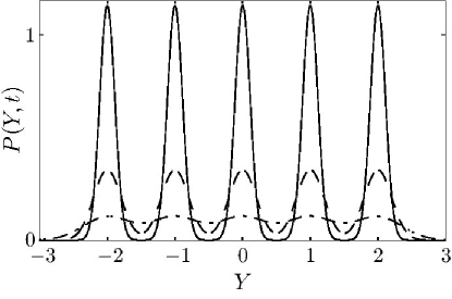
Figure 1: Here we show the probability density for the result of a measurement of the $z$-component of angular momentum for $j=2$, and with measurement strength $k$. This density is shown for three different measurement times: dot-dashed line: $t=1/k$; dashed line: $t=3/k$; solid line: $t=10/k$.

The random variable $Y$ has a physical meaning. Since we replaced the measurement record $dy$ by $dW/\sqrt{8k}$ to obtain the linear equation, when we transform from the raw probability density $\tilde{P}$ to the true density $P$ this transforms the driving noise process $dW$ back into $\sqrt{8k}\,dy=\sqrt{8k}\langle X(t)\rangle dt+dW$, being a scaled version of the measurement record. Thus, $Y(t)$, as we have defined it, is actually the output record up until time $t$, divided by $t$. That is,

$$Y=\frac{1}{t}\int_{0}^{t}\langle J_{z}(t)\rangle dt+\frac{1}{\sqrt{8k}\,t}\int_{0}^{t}dW.$$ (66)

Thus, $Y$ is the measurement result. When making the measurement the observer integrates up the measurement record, and then divides the result by the final time. The result is $Y$, and the closer $Y$ is to one of the eigenvalues, and the longer the time of the measurement, the more certain the observer is that the system has been collapsed onto the eigenstate with that eigenvalue. Note that as the measurement progresses, the second, explicitly stochastic term converges to zero, while the expectation value in the first term evolves to the measured eigenvalue.

VII Multiple Observers and Inefficient Detection

It is not difficult to extend the above analysis to describe what happens when more than one observer is monitoring the system. Consider two observers Alice and Bob, who measure the same system. Alice monitors $X$ with strength $k$, and Bob monitors $Y$ with strength $\kappa$. From Alice’s point of view, since she has no access to Bob’s measurement results, she must average over them. Thus, as far as Alice is concerned, Bob’s measurement simply induces the dynamics $d\rho_{1}=-\kappa[Y,[Y,\rho_{1}]]$ where $\rho_{1}$ is her state of knowledge. The full dynamics of her state of knowledge, including her measurement, evolves according to

$$\begin{array}[]{rcl}d\rho_{1}&{}={}&\displaystyle-k[X[X,\rho_{1}]]dt-\kappa[Y[Y,\rho_{1}]]dt\\ &&\displaystyle{}+\sqrt{2k}(X\rho_{1}+\rho_{1}X-2\langle X\rangle_{1}\rho_{1})dW_{1},\end{array}$$ (67)

where $\!\left\langle{X}\right\rangle_{1}:=\mathrm{Tr}[X\rho_{1}]$, and her measurement record is $dr_{1}=\!\left\langle{X}\right\rangle_{1}dt+dW_{1}/\sqrt{8k}$. Similarly, the equation of motion for Bob’s state of knowledge is

$$\begin{array}[]{rcl}d\rho_{2}&{}={}&\displaystyle-\kappa[Y[Y,\rho_{2}]]dt-k[X[X,\rho_{2}]]dt\\ &&\displaystyle+\sqrt{2\kappa}(Y\rho_{2}+\rho_{2}Y-2\langle Y\rangle_{2}\rho_{2})dW_{2},\end{array}$$ (68)

and his measurement record is $dr_{2}=\!\left\langle{Y}\right\rangle_{2}dt+dW_{2}/\sqrt{8\kappa}$.

We can also consider the state of knowledge of a single observer, Charlie, who has access to both measurement records $dr_{1}$ and $dr_{2}$. The equation for Charlie’s state of knowledge, $\rho$, is obtained simply by applying both measurements simultaneously, giving

$$\begin{array}[]{rcl}d\rho&{}={}&\displaystyle-k[X[X,\rho]]dt+\sqrt{2k}\left(X\rho+\rho X-2\langle X\rangle\rho\right)dV_{1}\\ &&\displaystyle{}-\kappa[Y[Y,\rho]]dt+\sqrt{2\kappa}\left(Y\rho+\rho Y-2\langle Y\rangle\rho\right)dV_{2},\end{array}$$ (69)

where $\!\left\langle{X}\right\rangle:=\mathrm{Tr}[X\rho]$. Note that $dV_{1}$ and $dV_{2}$ are independent noise sources. In terms of Charlie’s state of knowledge the two measurement records are

$$\begin{array}[]{rcl}dr_{1}&{}={}&\displaystyle\!\left\langle{X}\right\rangle dt+\frac{dV_{1}}{\sqrt{8k}},\\ dr_{2}&{}={}&\displaystyle\!\left\langle{Y}\right\rangle dt+\frac{dV_{2}}{\sqrt{8\kappa}}.\end{array}$$ (70)

In general Charlie’s state of knowledge $\rho(t)\not=\rho_{1}(t)\not=\rho_{2}(t)$, but Charlie’s measurement records are the same as Alice’s and Bob’s. Equating Charlie’s expressions for the measurement records with Alice’s and Bob’s, we obtain the relationship between Charlie’s noise sources and those of Alice and Bob:

$$\begin{array}[]{rcl}dV_{1}&{}={}&\displaystyle\sqrt{8k}\left(\,\!\left\langle{X}\right\rangle_{1}-\!\left\langle{X}\right\rangle\right)dt+dW_{1},\\ dV_{2}&{}={}&\displaystyle\sqrt{8\kappa}\left(\,\!\left\langle{Y}\right\rangle_{2}-\!\left\langle{Y}\right\rangle\right)dt+dW_{2}.\end{array}$$ (71)

We note that in quantum optics, each measurement is often referred to as a separate “output channel” for information, and so multiple simultaneous measurements are referred to as multiple output channels. Multiple observers were first treated explicitly by Barchielli, who gives a rigorous and mathematically sophisticated treatment in Ref. Barchielli (1993). A similarly detailed and considerably more accessible treatment is given in Ref. Dziarmaga et al. (2004).

We turn now to inefficient measurements, which can be treated in the same way as multiple observers. An inefficient measurement is one in which the observer is not able to pick up all the measurement signal. The need to consider inefficient measurements arose originally in quantum optics, where photon counters will only detect some fraction of the photons incident upon them. This fraction, usually denoted by $\eta$, is referred to as the efficiency of the detector Wiseman and Milburn (1993a). A continuous measurement in which the detector is inefficient can be described by treating the single measurement as two measurements, where the strengths of each of them sum to the strength of the single measurement. Thus we rewrite the equation for a measurement of $X$ at strength $k$ as

$$\begin{array}[]{rcl}d\rho&{}={}&\displaystyle-k_{1}[X[X,\rho]]\,dt+\sqrt{2k_{1}}(X\rho+\rho X-2\langle X\rangle\rho)\,dV_{1}\\ &&\displaystyle-k_{2}[X[X,\rho]]\,dt+\sqrt{2k_{2}}(X\rho+\rho X-2\langle X\rangle\rho)\,dV_{2},\end{array}$$ (72)

where $k_{1}+k_{2}=k$. We now give the observer access to only the measurement with strength $k_{1}$. From our discussion above, the equation for the observer’s state of knowledge, $\rho_{1}$, is

$$\begin{array}[]{rcl}d\rho_{1}&{}={}&\displaystyle-(k_{1}+k_{2})[X[X,\rho_{1}]]\,dt\\ &&\displaystyle{}+\sqrt{2k_{1}}(X\rho_{1}+\rho_{1}X-2\langle X\rangle_{1}\rho_{1})\,dW_{1}\\ &{}={}&\displaystyle-k[X[X,\rho_{1}]]\,dt+\\ &&\displaystyle\sqrt{2\eta k}(X\rho_{1}+\rho_{1}X-2\langle X\rangle_{1}\rho_{1})\,dW_{1},\end{array}$$ (73)

where, as before, the measurement record is

$$dr_{1}=\!\left\langle{X}\right\rangle_{1}dt+\frac{dW_{1}}{\sqrt{8k_{1}}}=\!\left\langle{X}\right\rangle_{1}dt+\frac{dW_{1}}{\sqrt{8\eta k}},$$ (74)

and

$$\eta=\frac{k_{1}}{k_{1}+k_{2}}=\frac{k_{1}}{k}$$ (75)

is the efficiency of the detector.

VIII General Form of the Stochastic Master Equation

Before looking at a physical example of a continuous measurement process, it is interesting to ask, what is the most general form of the measurement master equation when the measurements involve Gaussian noise? In this section we present a simplified version of an argument by Adler Adler (2000) that allows one to derive a form that is close to the fully general one and sufficient for most purposes. We also describe briefly the extension that gives the fully general form, the details of which have been worked out by Wiseman and Diosi Wiseman and Diosi (2001).

Under unitary (unconditioned) evolution, the Schrödinger equation tells us that in a short time interval $dt$, the state vector undergoes the transformation

$$|{\psi}\rangle\longrightarrow|{\psi}\rangle+d|{\psi}\rangle=\left(1-i\frac{H}{\hbar}\,dt\right)|{\psi}\rangle,$$ (76)

where $H$ is the Hamiltonian. The same transformation applied to the density operator gives the Schrödinger–von Neumann equation of Eq. (3):

$$\rho+d\rho=\left(1-i\frac{H}{\hbar}\,dt\right)\rho\left(1+i\frac{H}{\hbar}\,dt\right)=\rho-\frac{i}{\hbar}[H,\rho]\,dt.$$ (77)

To be physical, any transformation of the density operator must be completely positive. That is, the transformation must preserve the fact that the density operator has only nonnegative eigenvalues. This property guarantees that the density operator can generate only sensible (nonnegative) probabilities. (To be more precise, complete positivity means that the transformation for a system’s density operator must preserve the positivity of the density operator—the fact that the density operator has no negative eigenvalues—of any larger system containing the system Nielsen and Chuang (2000).) It turns out that the most general form of a completely positive transformation is

$$\rho\longrightarrow\sum_{n}A_{n}\rho A_{n}^{\dagger},$$ (78)

where the $A_{n}$ are arbitrary operators. The Hamiltonian evolution above corresponds to a single infinitesimal transformation operator $A=1-iH\,dt/\hbar$.

Now let’s examine the transformation for a more general, stochastic operator of the form

$$A=1-i\frac{H}{\hbar}\,dt+b\,dt+c\,dW,$$ (79)

where $b$ and $c$ are operators. We will use this operator to “derive” a Markovian master equation, then indicate how it can be made more general. We may assume here that $b$ is Hermitian, since we can absorb any antihermitian part into the Hamiltonian. Putting this into the transformation (78), we find

$$d\rho=-\,\frac{i}{\hbar}[H,\rho]\,dt+[b,\rho]_{+}dt+c\rho c^{\dagger}\,dt+\left(c\rho+\rho c^{\dagger}\right)\,dW,$$ (80)

where $[A,B]_{+}:=AB+BA$ is the anticommutator. We can then take an average over all possible Wiener processes, which again we denote by the double angle brackets $\left\langle\!\left\langle{~{}}\right\rangle\!\right\rangle$. From Eq. (52), $\left\langle\!\left\langle{\rho\,dW}\right\rangle\!\right\rangle=0$ in Itô calculus, so

$$d\left\langle\!\left\langle{\rho}\right\rangle\!\right\rangle=-\,\frac{i}{\hbar}\left[H,\left\langle\!\left\langle{\rho}\right\rangle\!\right\rangle\right]\,dt+\left[b,\left\langle\!\left\langle{\rho}\right\rangle\!\right\rangle\right]_{+}dt+c\left\langle\!\left\langle{\rho}\right\rangle\!\right\rangle\!c^{\dagger}\,dt.$$ (81)

Since the operator $\left\langle\!\left\langle{\rho}\right\rangle\!\right\rangle$ is an average over valid density operators, it is also a valid density operator and must therefore satisfy $\mathrm{Tr}[\left\langle\!\left\langle{\rho}\right\rangle\!\right\rangle]=1$. Hence we must have $d\mathrm{Tr}[\left\langle\!\left\langle{\rho}\right\rangle\!\right\rangle]=\mathrm{Tr}[d\!\left\langle\!\left\langle{\rho}\right\rangle\!\right\rangle]=0$. Using the cyclic property of the trace, this gives

$$\mathrm{Tr}\left[\left\langle\!\left\langle{\rho}\right\rangle\!\right\rangle\left(2b+c^{\dagger}c\right)\right]=0.$$ (82)

This holds for an arbitrary density operator only if

$$b=-\,\frac{c^{\dagger}c}{2}.$$ (83)

Thus we obtain the Lindblad form Lindblad (1976) of the master equation (averaged over all possible noise realizations):

$$d\left\langle\!\left\langle{\rho}\right\rangle\!\right\rangle=-\,\frac{i}{\hbar}\left[H,\left\langle\!\left\langle{\rho}\right\rangle\!\right\rangle\right]\,dt+\mathcal{D}[c]\!\left\langle\!\left\langle{\rho}\right\rangle\!\right\rangle\,dt.$$ (84)

Here, we have defined the Lindblad superoperator

$$\mathcal{D}[c]\rho:=c\rho c^{\dagger}-\frac{1}{2}\left(c^{\dagger}c\rho+\rho c^{\dagger}c\right),$$ (85)

where “superoperator” refers to the fact that $\mathcal{D}[c]$ operates on $\rho$ from both sides. This is the most general (Markovian) form of the unconditioned master equation for a single dissipation process.

The full transformation from Eq. (80) then becomes

$$d\rho=-\,\frac{i}{\hbar}[H,\rho]\,dt+\mathcal{D}[c]\rho\,dt+\left(c\rho+\rho c^{\dagger}\right)\,dW.$$ (86)

This is precisely the linear master equation, for which we already considered the special case of $c=\sqrt{2k}X$ for the measurement parts in Eq. (58). Again, this form of the master equation does not in general preserve the trace of the density operator, since the condition $\mathrm{Tr}[d\rho]=0$ implies

$$\mathrm{Tr}\left[\rho\left(c+c^{\dagger}\right)\,dW\right]=0.$$ (87)

We could interpret this relation as a constraint on $c$ Adler (2000), but we will instead keep $c$ an arbitrary operator and explicitly renormalize $\rho$ at each time step by adding a term proportional to the left-hand side of (87). The result is the nonlinear form

$$d\rho=-\,\frac{i}{\hbar}[H,\rho]\,dt+\mathcal{D}[c]\rho\,dt+\mathcal{H}[c]\rho\,dW,$$ (88)

where the measurement superoperator is

$$\mathcal{H}[c]\rho:=c\rho+\rho c^{\dagger}-\!\left\langle{c+c^{\dagger}}\right\rangle\rho.$$ (89)

When $c$ is Hermitian, the measurement terms again give precisely the stochastic master equation (32).

More generally, we may have any number of measurements, sometimes referred to as output channels, happening simultaneously. The result is

$$d\rho=-\,\frac{i}{\hbar}[H,\rho]\,dt+\sum_{n}\left(\mathcal{D}[c_{n}]\rho\,dt+\mathcal{H}[c_{n}]\rho\,dW_{n}\right).$$ (90)

This is the same as Eq. (88), but this time summed (integrated) over multiple possible measurement operators $c_{n}$, each with a separate Wiener noise process independent of all the others.

In view of the arguments of Section (VII), when the measurements are inefficient, we have

$$d\rho=-\,\frac{i}{\hbar}[H,\rho]\,dt+\sum_{n}\left(\mathcal{D}[c_{n}]\rho\,dt,+\sqrt{\eta_{n}}\mathcal{H}[c_{n}]\rho\,dW\right),$$ (91)

where $\eta_{n}$ is the efficiency of the $n$th detection channel. The corresponding measurement record for the $n$th process can be written

$$dr(t)=\frac{\!\left\langle{c_{n}+c_{n}^{\dagger}}\right\rangle}{2}dt+\frac{dW_{n}}{\sqrt{4\eta_{n}}}.$$ (92)

Again, for a single, position-measurement channel of the form $c=\sqrt{2k}X$, we recover Eqs. (31) and (74) if we identify $dr_{n}/\sqrt{2k}$ as a rescaled measurement record.

The SME in Eq. (91) is sufficiently general for most purposes when one is concerned with measurements resulting in Wiener noise, but is not quite the most general form for an SME driven by such noise. The most general form is worked out in Ref. Wiseman and Diosi (2001), and includes the fact that the noise sources may also be complex and mutually correlated.

IX Interpretation of the Master Equation

Though we now have the general form of the master equation (91), the interpretation of each of the measurement terms is not entirely obvious. In particular, the $\mathcal{H}[c]\rho$ terms (i.e., the noise terms) represent the information gain due to the measurement process, while the $\mathcal{D}[c]\rho$ terms represent the disturbance to, or the backaction on, the state of the system due to the measurement. Of course, as we see from the dependence on the efficiency $\eta$, the backaction occurs independently of whether the observer uses or discards the measurement information (corresponding to $\eta=1$ or $0$, respectively).

To examine the roles of these terms further, we will now consider the equations of motion for the moments (expectation values of powers of $X$ and $P$) of the canonical variables. In particular, we will specialize to the case of a single measurement channel,

$$d\rho=-\,\frac{i}{\hbar}[H,\rho]\,dt+\mathcal{D}[c]\rho\,dt+\sqrt{\eta}\mathcal{H}[c]\rho\,dW.$$ (93)

For an arbitrary operator $A$, we can use the master equation and $d\!\left\langle{A}\right\rangle=\mathrm{Tr}[A\,d\rho]$ to obtain following equation of motion for the expectation value $\!\left\langle{A}\right\rangle$:

$$\begin{array}[]{rcl}d\!\left\langle{A}\right\rangle&{}={}&\displaystyle-\,\frac{i}{\hbar}\!\left\langle{[A,H]}\right\rangle\,dt\\ &&\displaystyle+\!\left\langle{c^{\dagger}Ac-\frac{1}{2}\left(c^{\dagger}cA+Ac^{\dagger}c\right)}\right\rangle\,dt\\ &&\displaystyle{}+\sqrt{\eta}\!\left\langle{c^{\dagger}A+Ac-\!\left\langle{A}\right\rangle\!\left\langle{c+c^{\dagger}}\right\rangle}\right\rangle\,dW.\end{array}$$ (94)

Now we will consider the effects of measurements on the relevant expectation values in two example cases: a position measurement, corresponding to an observable, and an antihermitian operator, corresponding to an energy damping process. As we will see, the interpretation differs slightly in the two cases. For concreteness and simplicity, we will assume the system is a harmonic oscillator of the form

$$H=\frac{P^{2}}{2m}+\frac{1}{2}m\omega_{0}^{\,2}X^{2},$$ (95)

and consider the lowest few moments of $X$ and $P$. We will also make the simplifying assumption that the initial state is Gaussian, so that we only need to consider the simplest five moments: the means  $\!\left\langle{X}\right\rangle$ and $\!\left\langle{P}\right\rangle$, the variances $V_{X}$ and $V_{P}$, where $V_{\alpha}:=\!\left\langle{\alpha^{2}}\right\rangle-\!\left\langle{\alpha}\right\rangle^{2}$, and the symmetrized covariance $C_{XP}:=(1/2)\!\left\langle{[X,P]_{+}}\right\rangle-\!\left\langle{X}\right\rangle\!\left\langle{P}\right\rangle$. These moments completely characterize arbitrary Gaussian states (including mixed states).

IX.1 Position Measurement

In the case of a position measurement of the form $c=\sqrt{2k}\,X$ as in Eq. (58), Eq. (94) becomes

$$\begin{array}[]{rcl}d\!\left\langle{A}\right\rangle&{}={}&\displaystyle-\,\frac{i}{\hbar}\!\left\langle{[A,H]}\right\rangle\,dt-k\!\left\langle{[X,[X,A]]}\right\rangle\,dt\\ &&\displaystyle{}+\sqrt{2\eta k}\left[\!\left\langle{[X,A]_{+}}\right\rangle-2\!\left\langle{X}\right\rangle\!\left\langle{A}\right\rangle\right]\,dW.\end{array}$$ (96)

Using this equation to compute the cumulant equations of motion, we find Doherty and Jacobs (1999)

$$\begin{array}[]{rcl}d\!\left\langle{X}\right\rangle&{}={}&\displaystyle\frac{1}{m}\!\left\langle{P}\right\rangle\,dt+\sqrt{8\eta k}V_{X}\,dW\\ d\!\left\langle{P}\right\rangle&{}={}&\displaystyle-m\omega_{0}^{\,2}\!\left\langle{X}\right\rangle\,dt+\sqrt{8\eta k}C_{XP}\,dW\\ \partial_{t}V_{X}&{}={}&\displaystyle\frac{2}{m}C_{XP}-8\eta kV_{X}^{\,2}\\ \partial_{t}V_{P}&{}={}&\displaystyle-2m\omega_{0}^{\,2}C_{XP}+2\hbar^{2}k-8\eta kC_{XP}^{\,2}\\ \partial_{t}C_{XP}&{}={}&\displaystyle\frac{1}{m}V_{P}-m\omega_{0}^{\,2}V_{X}-8\eta kV_{X}C_{XP}.\end{array}$$ (97)

Notice that in the variance equations, the $dW$ terms vanished, due to the assumption of a Gaussian state, which implies the following relations for the moments Habib (2004):

$$\begin{array}[]{rcl}\!\left\langle{X^{3}}\right\rangle&{}={}&\displaystyle\!\left\langle{X}\right\rangle^{3}+3\!\left\langle{X}\right\rangle V_{X}\\ \displaystyle\frac{1}{2}\!\left\langle{[X,P^{2}]_{+}}\right\rangle&{}={}&\displaystyle\!\left\langle{X}\right\rangle\!\left\langle{P}\right\rangle^{2}+2\!\left\langle{P}\right\rangle C_{XP}+\!\left\langle{X}\right\rangle V_{P}\\ \displaystyle\frac{1}{2}\!\left\langle{[X,[X,P]_{+}]_{+}}\right\rangle&{}={}&\displaystyle\!\left\langle{X}\right\rangle\!\left\langle{P}\right\rangle^{2}+2\!\left\langle{X}\right\rangle C_{XP}+\!\left\langle{P}\right\rangle V_{X}.\end{array}$$ (98)

For the reader wishing to become better acquainted with continuous measurement theory, the derivation of Eqs. (97) is an excellent exercise. The derivation is straightforward, the only subtlety being the second-order Itô terms in the variances. For example, the equation of motion for the position variance starts as

$$dV_{X}=d\!\left\langle{X^{2}}\right\rangle-2\!\left\langle{X}\right\rangle d\!\left\langle{X}\right\rangle-(d\!\left\langle{X}\right\rangle)^{2}.$$ (99)

The last, quadratic term is important in producing the effect that the measured quantity becomes more certain.

In examining Eqs. (97), we can simply use the coefficients to identify the source and thus the interpretation of each term. The first term in each equation is due to the natural Hamiltonian evolution of the harmonic oscillator. Terms originating from the $\mathcal{D}[c]\rho$ component are proportional to $k\,dt$ but not $\eta$; in fact, the only manifestation of this term is the $\hbar^{2}k$ term in the equation of motion for $V_{P}$. Thus, a position measurement with rate constant $k$ produces momentum diffusion (heating) at a rate $\hbar^{2}k$, as is required to maintain the uncertainty principle as the position uncertainty contracts due to the measurement.

There are more terms here originating from the $\mathcal{H}[c]\rho$ component of the master equation, and they are identifiable since they are proportional to either $\sqrt{\eta k}$ or $\eta k$. The $dW$ terms in the equations for $\!\left\langle{X}\right\rangle$ and $\!\left\langle{P}\right\rangle$ represent the stochastic nature of the position measurement. That is, during each small time interval, the wave function collapses slightly, but we don’t know exactly where it collapses to. This stochastic behavior is precisely the same behavior that we saw in Eq. (26). The more subtle point here lies with the nonstochastic terms proportional to $\eta k$, which came from the second-order term [for example, in Eq. (99)] where Itô calculus generates a nonstochastic term from $dW^{2}=dt$. Notice in particular the term of this form in the $V_{X}$ equation, which acts as a damping term for $V_{X}$. This term represents the certainty gained via the measurement process. The other similar terms are less clear in their interpretation, but they are necessary to maintain consistency of the evolution.

Note that we have made the assumption of a Gaussian initial state in deriving these equations, but this assumption is not very restrictive. Due to the linear potential and the Gaussian POVM for the measurement collapse, these equations of motion preserve the Gaussian form of the initial state. The Gaussian POVM additionally converts arbitrary initial states into Gaussian states at long times. Furthermore, the assumption of a Gaussian POVM is not restrictive—under the assumption of sufficiently high noise bandwidth, the central-limit theorem guarantees that temporal coarse-graining yields Gaussian noise for any POVM giving random deviates with bounded variance.

IX.2 Dissipation

The position measurement above is an example of a Hermitian measurement operator. But what happens when the measurement operator is antihermitian? As an example, we will consider the annihilation operator for the harmonic oscillator by setting $c=\sqrt{\gamma}\,a$, where

$$a=\frac{1}{\sqrt{2}x_{0}}X+i\frac{x_{0}}{\sqrt{2}\hbar}P$$ (100)

and

$$x_{0}:=\sqrt{\frac{\hbar}{m\omega_{0}}}.$$ (101)

The harmonic oscillator with this type of measurement models, for example, the field of an optical cavity whose output is monitored via homodyne detection, where the cavity output is mixed on a beamsplitter with another optical field. (Technically, in homodyne detection, the field must be the same as the field driving the cavity; mixing with other fields corresponds to heterodyne detection.) A procedure very similar to the one above gives the following cumulant equations for the conditioned evolution in this case:

$$\begin{array}[]{rcl}d\!\left\langle{X}\right\rangle&{}={}&\displaystyle\frac{1}{m}\!\left\langle{P}\right\rangle\,dt-\frac{\gamma}{2}\!\left\langle{X}\right\rangle\,dt\\ &&\displaystyle{}+\sqrt{2\eta\gamma\frac{m\omega_{0}}{\hbar}}\left(V_{X}-\frac{\hbar}{2m\omega_{0}}\right)dW\\ d\!\left\langle{P}\right\rangle&{}={}&\displaystyle-m\omega_{0}^{\,2}\!\left\langle{X}\right\rangle\,dt-\frac{\gamma}{2}\!\left\langle{P}\right\rangle\,dt\\ &&\displaystyle{}+\sqrt{2\eta\gamma\frac{m\omega_{0}}{\hbar}}C_{XP}\,dW\\ \partial_{t}V_{X}&{}={}&\displaystyle\frac{2}{m}C_{XP}-\gamma\left(V_{X}-\frac{\hbar}{2m\omega_{0}}\right)\\ &&\displaystyle{}-2\eta\gamma\frac{m\omega_{0}}{\hbar}\left(V_{X}-\frac{\hbar}{2m\omega_{0}}\right)^{2}\\ \partial_{t}V_{P}&{}={}&\displaystyle-m\omega_{0}^{\,2}C_{XP}-\gamma\left(V_{P}-\frac{m\omega_{0}\hbar}{2}\right)\\ &&\displaystyle{}-2\eta\gamma\frac{m\omega_{0}}{\hbar}C_{XP}^{\,2}\\ \partial_{t}C_{XP}&{}={}&\displaystyle\frac{1}{m}V_{P}-m\omega_{0}^{\,2}V_{X}-\gamma C_{XP}\\ &&\displaystyle{}-2\eta\gamma\frac{m\omega_{0}}{\hbar}C_{XP}\left(V_{X}-\frac{\hbar}{2m\omega_{0}}\right).\end{array}$$ (102)

The moment equations seem more complex in this case, but are still fairly simple to interpret.

First, consider the unconditioned evolution of the means $\!\left\langle{X}\right\rangle$ and $\!\left\langle{P}\right\rangle$, where we average over all possible noise realizations. Again, since $\left\langle\!\left\langle{\rho\,dW}\right\rangle\!\right\rangle=0$, we can simply set $dW=0$ in the above equations, and we will drop the double angle brackets for brevity. The Hamiltonian evolution terms are of course the same, but now we see extra damping terms. Decoupling these two equations gives an equation of the usual form for the damped harmonic oscillator for the mean position:

$$\partial_{t}^{\,2}{\!\left\langle{X}\right\rangle}+\gamma\partial_{t}{\!\left\langle{X}\right\rangle}+\left(\omega_{0}^{\,2}+\frac{\gamma^{2}}{4}\right)\!\left\langle{X}\right\rangle=0.$$ (103)

Note that we identify the frequency $\omega_{0}$ here as the actual oscillation frequency $\omega_{\gamma}$ of the damped oscillator, given by $\omega_{\gamma}^{\,2}=\omega_{0}^{\,2}-\gamma^{2}/4$, and not the resonance frequency $\omega_{0}$ that appears the usual form of the classical formula.

The noise terms in these equations correspond to nonstationary diffusion, or diffusion where the transport rate depends on the state of the system. Note that under such a diffusive process, the system will tend to come to rest in configurations where the diffusion coefficient vanishes, an effect closely related to the “blowtorch theorem” Landauer (1993). Here, this corresponds to $V_{X}=\hbar/2m\omega_{0}$ and $C_{XP}=0$.

The variance equations also contain unconditioned damping terms (proportional to $\gamma$ but not $\eta$). These damping terms cause the system to equilibrate with the same variance values as noted above; they also produce the extra equilibrium value $V_{P}=m\omega_{0}\hbar/2$. The conditioning terms (proportional to $\eta$) merely accelerate the settling to the equilibrium values. Thus, we see that the essential effect of the antihermitian measurement operator is to damp the energy from the system, whether it is stored in the centroids or in the variances. In fact, what we see is that this measurement process selects coherent states, states that have the same shape as the harmonic-oscillator ground state, but whose centroids oscillate along the classical harmonic-oscillator trajectories.

X Physical Model of a Continuous Measurement: Atomic Spontaneous Emission

To better understand the nature of continuous measurements, we will now consider in detail an example of how a continuous measurement of position arises in a fundamental physical system: a single atom interacting with light. Again, to obtain weak measurements, we do not make projective measurements directly on the atom, but rather we allow the atom to become entangled with an auxiliary quantum system—in this case, the electromagnetic field—and then make projective measurements on the auxiliary system (in this case, using a photodetector). It turns out that this one level of separation between the system and the projective measurement is the key to the structure of the formalism. Adding more elements to the chain of quantum-measurement devices does not change the fundamental structure that we present here.

X.1 Master Equation for Spontaneous Emission

We begin by considering the interaction of the atom with the electromagnetic field. In particular, treating the field quantum mechanically allows us to treat spontaneous emission. These spontaneously emitted photons can then be detected to yield information about the atom.

X.1.1 Decay of the Excited State

We will give a brief treatment following the approach of Weisskopf and Wigner Weisskopf and Wigner (1930); Scully and Zubairy (1997); Milonni (1994). Without going into detail about the quantization of the electromagnetic field, we will simply note that the quantum description of the field involves associating a quantum harmonic oscillator with each field mode (say, each plane wave of a particular wave vector $\mathbf{k}$ and definite polarization). Then for a two-level atom with ground and excited levels $|{\mathrm{g}}\rangle$ and $|{\mathrm{e}}\rangle$, respectively, the uncoupled Hamiltonian for the atom and a single field mode is

$$H_{0}=\hbar\omega_{0}\sigma^{\dagger}\sigma+\hbar\omega\left(a^{\dagger}a+\frac{1}{2}\right).$$ (104)

Here, $\omega_{0}$ is the transition frequency of the atom, $\omega$ is the frequency of the field mode, $\sigma:=|{\mathrm{g}}\rangle\langle{\mathrm{e}}|$ is the atomic lowering operator (so that $\sigma^{\dagger}\sigma=|{\mathrm{e}}\rangle\langle{\mathrm{e}}|$ is the excited-state projector), and $a$ is the field (harmonic oscillator) annihilation operator. The interaction between the atom and field is given in the dipole and rotating-wave approximations by the interaction Hamiltonian

$$H_{\mathrm{\scriptscriptstyle AF}}=\hbar\left(g\sigma^{\dagger}a+g^{*}\sigma a^{\dagger}\right),$$ (105)

where $g$ is a coupling constant that includes the volume of the mode, the field frequency, and the atomic dipole moment. The two terms here are the “energy-conserving” processes corresponding to photon absorption and emission.

In the absence of externally applied fields, we can write the state vector as the superposition of the states

$${|\psi\rangle}=c_{\mathrm{e}}|{\mathrm{e}}\rangle+c_{\mathrm{g}}|{\mathrm{g},1}\rangle,$$ (106)

where the uncoupled eigenstate $|{\alpha,n}\rangle$ denotes the atomic state $|{\alpha}\rangle$ and the $n$-photon field state, and the omitted photon number denotes the vacuum state: $|{\alpha}\rangle\equiv|{\alpha,0}\rangle$. These states form an effectively complete basis, since no other states are coupled to these by the interaction (105). We will also assume that the atom is initially excited, so that $c_{\mathrm{e}}(0)=1$ and $c_{\mathrm{g}}(0)=0$.

The evolution is given by the Schrödinger equation,

$$\partial_{t}{|\psi\rangle}=-\,\frac{i}{\hbar}(H_{0}+H_{\mathrm{\scriptscriptstyle AF}}){|\psi\rangle},$$ (107)

which gives, upon substitution of (106) and dropping the vacuum energy offset of the field,

$$\begin{array}[]{rcl}\partial_{t}c_{\mathrm{e}}&{}={}&\displaystyle-i\omega_{0}c_{\mathrm{e}}-igc_{\mathrm{g}}\\ \partial_{t}c_{\mathrm{g}}&{}={}&\displaystyle-i\omega c_{\mathrm{g}}-ig^{*}c_{\mathrm{e}}.\end{array}$$ (108)

Defining the slowly varying amplitudes $\tilde{c}_{\mathrm{e}}:=c_{\mathrm{e}}e^{i\omega_{0}t}$ and $\tilde{c}_{\mathrm{g}}:=c_{\mathrm{g}}e^{i\omega t}$, we can rewrite these as

$$\begin{array}[]{rcl}\partial_{t}\tilde{c}_{\mathrm{e}}&{}={}&\displaystyle-ig\tilde{c}_{\mathrm{g}}e^{-i(\omega-\omega_{0})t}\\ \partial_{t}\tilde{c}_{\mathrm{g}}&{}={}&\displaystyle-ig^{*}\tilde{c}_{\mathrm{e}}e^{i(\omega-\omega_{0})t}.\end{array}$$ (109)

To decouple these equations, we first integrate the equation for $\tilde{c}_{\mathrm{g}}$:

$$\tilde{c}_{\mathrm{g}}(t)=-ig^{*}\int_{0}^{t}dt^{\prime}\,\tilde{c}_{\mathrm{e}}(t^{\prime})e^{i(\omega-\omega_{0})t^{\prime}}.$$ (110)

Substituting this into the equation for $\tilde{c}_{\mathrm{e}}$,

$$\partial_{t}\tilde{c}_{\mathrm{e}}=-|g|^{2}\int_{0}^{t}dt^{\prime}\,\tilde{c}_{\mathrm{e}}(t^{\prime})e^{-i(\omega-\omega_{0})(t-t^{\prime})},$$ (111)

which gives the evolution for the excited state coupled to a single field mode.

Now we need to sum over all field modes. In free space, we can integrate over all possible plane waves, labeled by the wave vector $\mathbf{k}$ and the two possible polarizations $\zeta$ for each wave vector. Each mode has a different frequency $\omega_{\mathbf{k}}=ck$, and we must expand the basis so that a photon can be emitted into any mode:

$${|\psi\rangle}=c_{\mathrm{e}}|{\mathrm{e}}\rangle+\sum_{\mathbf{k},\zeta}c_{\mathbf{k},\zeta}{|\mathrm{g},1_{\mathrm{k},\zeta}\rangle}.$$ (112)

Putting in the proper form of the coupling constants $g_{\mathbf{k}}$ for each mode in the free-space limit, it turns out that the equation of motion becomes

$$\begin{array}[]{l}\displaystyle\partial_{t}\tilde{c}_{\mathrm{e}}=\\ \displaystyle-\,\frac{d_{\mathrm{ge}}^{2}}{6\epsilon_{0}\hbar(2\pi)^{3}}\sum_{\zeta}\int d\mathbf{k}\,\omega_{\mathbf{k}}\displaystyle\int_{0}^{t}dt^{\prime}\,\tilde{c}_{\mathrm{e}}(t^{\prime})e^{-i(\omega_{\mathbf{k}}-\omega_{0})(t-t^{\prime})},\end{array}$$ (113)

where $\mathbf{d}_{\mathrm{ge}}:=\langle{\mathrm{g}}|\mathbf{d}|{\mathrm{e}}\rangle$ is the dipole matrix element characterizing the atomic transition strength. The polarization sum simply contributes a factor of 2, while carrying out the angular integration in spherical coordinates gives

$$\partial_{t}\tilde{c}_{\mathrm{e}}=-\,\frac{d_{\mathrm{ge}}^{2}}{6\pi^{2}\epsilon_{0}\hbar c^{3}}\int_{0}^{\infty}\!\!d\omega\,\omega^{3}\int_{0}^{t}dt^{\prime}\,\tilde{c}_{\mathrm{e}}(t^{\prime})e^{-i(\omega_{\mathbf{k}}-\omega_{0})(t-t^{\prime})}.$$ (114)

We can now note that $\tilde{c}_{\mathrm{e}}(t^{\prime})$ varies slowly on optical time scales. Also, $\omega^{3}$ is slowly varying compared to the exponential factor in Eq. (114), which oscillates rapidly (at least for large times $t$) about zero except when $t\approx t^{\prime}$ and $\omega\approx\omega_{0}$. Thus, we will get a negligible contribution from the $\omega$ integral away from $\omega=\omega_{0}$. We will therefore make the replacement $\omega^{3}\longrightarrow\omega_{0}^{\,3}$:

$$\begin{array}[]{rcl}\partial_{t}\tilde{c}_{\mathrm{e}}&{}={}&\displaystyle-\frac{\omega_{0}^{\,3}d_{\mathrm{ge}}^{2}}{6\pi^{2}\epsilon_{0}\hbar c^{3}}\int_{0}^{\infty}d\omega\,\int_{0}^{t}dt^{\prime}\,\tilde{c}_{\mathrm{e}}(t^{\prime})e^{-i(\omega_{\mathbf{k}}-\omega_{0})(t-t^{\prime})}.\end{array}$$ (115)

The same argument gives

$$\begin{array}[]{rcl}\displaystyle\int_{0}^{\infty}d\omega\,e^{-i(\omega_{\mathbf{k}}-\omega_{0})(t-t^{\prime})}&{}\approx{}&\displaystyle\int_{-\infty}^{\infty}d\omega\,e^{-i(\omega_{\mathbf{k}}-\omega_{0})(t-t^{\prime})}\\ &{}={}&\displaystyle 2\pi\delta(t-t^{\prime}).\end{array}$$ (116)

We can see from this that our argument here about the exponential factor is equivalent to the Markovian approximation, where we assume that the time derivative of the quantum state depends only on the state at the present time. Thus,

$$\begin{array}[]{rcl}\partial_{t}\tilde{c}_{\mathrm{e}}&{}={}&\displaystyle-\frac{\omega_{0}^{\,3}d_{\mathrm{ge}}^{2}}{3\pi\epsilon_{0}\hbar c^{3}}\int_{0}^{t}dt^{\prime}\,\tilde{c}_{\mathrm{e}}(t^{\prime})\delta(t-t^{\prime})\\ &{}={}&\displaystyle-\frac{\omega_{0}^{\,3}d_{\mathrm{ge}}^{2}}{3\pi\epsilon_{0}\hbar c^{3}}\frac{\tilde{c}_{\mathrm{e}}(t)}{2}.\\ \end{array}$$ (117)

Here, we have split the $\delta$-function since the upper limit of the $t^{\prime}$ integral was $t$, in view of the original form (115) for the $t^{\prime}$ integral, where the integration limit is centered at the peak of the exponential factor. We can rewrite the final result as

$$\partial_{t}\tilde{c}_{\mathrm{e}}=-\,\frac{\Gamma}{2}\tilde{c}_{\mathrm{e}},$$ (118)

where the spontaneous decay rate is given by

$$\Gamma:=\frac{\omega_{0}^{\,3}d^{2}_{\mathrm{ge}}}{3\pi\epsilon_{0}\hbar c^{3}}.$$ (119)

This decay rate is of course defined so that the probability decays exponentially at the rate $\Gamma$. Also, note that

$$\partial_{t}c_{\mathrm{e}}=\left(-i\omega_{0}-\frac{\Gamma}{2}\right)c_{\mathrm{e}}$$ (120)

after transforming out of the slow variables.

X.1.2 Form of the Master Equation

We now want to consider the reduced density operator for the evolution of the atomic state, tracing over the state of the field. Here we will compute the individual matrix elements

$$\rho_{\alpha\beta}:=\!\left\langle{\alpha|\rho|\beta}\right\rangle$$ (121)

for the atomic state.

The easiest matrix element to treat is the excited-level population,

$$\rho_{\mathrm{ee}}=c_{\mathrm{e}}c_{\mathrm{e}}^{*}.$$ (122)

Differentiating this equation and using (118) gives

$$\partial_{t}\rho_{\mathrm{ee}}=-\Gamma\rho_{\mathrm{ee}}.$$ (123)

The matrix element for the ground-state population follows from summing over all the other states:

$$\rho_{\mathrm{gg}}:=\sum_{\zeta}\int d\mathrm{k}\,\tilde{c}_{\mathbf{k},\zeta}\tilde{c}_{\mathbf{k},\zeta}^{*}.$$ (124)

Notice that the states $|{\mathrm{e}}\rangle$ and $|{\mathrm{g}}\rangle$ are effectively degenerate, but when we eliminate the field, we want $|{\mathrm{e}}\rangle$ to have $\hbar\omega_{0}$ more energy than the ground state. The shortcut for doing this is to realize that the latter situation corresponds to the “interaction picture” with respect to the field, where we use the slowly varying ground-state amplitudes $\tilde{c}_{\mathbf{k},\zeta}$ but the standard excited-state amplitude $c_{\mathrm{e}}$. This explains why we use regular coefficients in Eq. (122) but the slow variables in Eq. (124). Since by construction $\rho_{\mathrm{ee}}+\rho_{\mathrm{gg}}=1$,

$$\partial_{t}\rho_{\mathrm{gg}}=\Gamma\rho_{\mathrm{ee}}.$$ (125)

Finally, the coherences are

$$\rho_{\mathrm{ge}}:=\sum_{\zeta}\int d\mathbf{k}\,\tilde{c}_{\mathbf{k},\zeta}c_{\mathrm{e}}^{*},\hskip 14.22636pt\rho_{\mathrm{eg}}=\rho_{\mathrm{ge}}^{*},$$ (126)

and so the corresponding equation of motion is

$$\partial_{t}\rho_{\mathrm{ge}}=\sum_{\zeta}\int d\mathbf{k}\,\tilde{c}_{\mathbf{k},\zeta}\left(i\omega_{0}-\frac{\Gamma}{2}\right)c_{\mathrm{e}}^{*}=\left(i\omega_{0}-\frac{\Gamma}{2}\right)\rho_{\mathrm{ge}}.$$ (127)

We have taken the time derivatives of the $\tilde{c}_{\mathbf{k},\zeta}$ to be zero here. From Eq. (109), the time derivatives, when summed over all modes, will in general correspond to a sum over amplitudes with rapidly varying phases, and thus their contributions will cancel.

Notice that what we have derived are exactly the same matrix elements generated by the master equation

$$\partial_{t}\rho=-\,\frac{i}{\hbar}[H_{\mathrm{\scriptscriptstyle A}},\rho]+\Gamma\mathcal{D}[\sigma]\rho,$$ (128)

where the form of $\mathcal{D}[\sigma]\rho$ is given by Eq. (85), and the atomic Hamiltonian is

$$H_{\mathrm{\scriptscriptstyle A}}:=\hbar\omega_{0}|{\mathrm{e}}\rangle\langle{\mathrm{e}}|.$$ (129)

That is, the damping term here represents the same damping as in the optical Bloch equations.

X.2 Photodetection: Quantum Jumps and the Poisson Process

In deriving Eq. (128), we have ignored the state of the field. Now we will consider what happens when we measure it. In particular, we will assume that we make projective measurements of the field photon number in every mode, not distinguishing between photons in different modes. It is this extra interaction that will yield the continuous measurement of the atomic state.

From Eq. (123), the transition probability in a time interval of length $dt$ is $\Gamma\rho_{\mathrm{ee}}\,dt=\Gamma\!\left\langle{\sigma^{\dagger}\sigma}\right\rangle dt$, where we recall that $\sigma^{\dagger}\sigma=|{\mathrm{e}}\rangle\langle{\mathrm{e}}|$ is the excited-state projection operator. Then assuming an ideal detector that detects photons at all frequencies, polarizations, and angles, there are two possibilities during this time interval:

1. No photon detected. The detector does not “click” in this case, and this possibility happens with probability $1-\Gamma\!\left\langle{\sigma^{\dagger}\sigma}\right\rangle dt$. The same construction as above for the master equation carries through, so we keep the equations of motion for $\rho_{\mathrm{ee}}$, $\rho_{\mathrm{eg}}$, and $\rho_{\mathrm{ge}}$. However, we do not keep the same equation for $\rho_{\mathrm{gg}}$: no photodetection implies that the atom does not return to the ground state. Thus, $\partial_{t}\rho_{\mathrm{gg}}=0$. This case is thus generated by the master equation

   $$\partial_{t}\rho=-\,\frac{i}{\hbar}[H_{\mathrm{\scriptscriptstyle A}},\rho]-\frac{\Gamma}{2}[\sigma^{\dagger}\sigma,\rho]_{+}.$$ (130)

   This evolution is unnormalized since $\mathrm{Tr}[\rho]$ decays to zero at long times. We can remedy this by explicitly renormalizing the state $\rho(t+dt)$, which amounts to adding one term to the master equation, as in Eq. (88):

   $$\partial_{t}\rho=-\,\frac{i}{\hbar}[H_{\mathrm{\scriptscriptstyle A}},\rho]-\frac{\Gamma}{2}[\sigma^{\dagger}\sigma,\rho]_{+}+\Gamma\!\left\langle{\sigma^{\dagger}\sigma}\right\rangle\rho.$$ (131)

2. Photon detected. A click on the photodetector occurs with probability $\Gamma\!\left\langle{\sigma^{\dagger}\sigma}\right\rangle dt$. The interaction Hamiltonian $H_{\mathrm{\scriptscriptstyle AF}}$ contains a term of the form $\sigma a^{\dagger}$, which tells us that photon creation (and subsequent detection) is accompanied by lowering of the atomic state. Thus, the evolution for this time interval is given by the reduction

   $$\rho(t+dt)=\frac{\sigma\rho(t)\sigma^{\dagger}}{\!\left\langle{\sigma^{\dagger}\sigma}\right\rangle}.$$ (132)

   We can write this in differential form as

   $$d\rho=\frac{\sigma\rho\sigma^{\dagger}}{\!\left\langle{\sigma^{\dagger}\sigma}\right\rangle}-\rho.$$ (133)

The overall evolution is stochastic, with either case occurring during a time interval $dt$ with the stated probabilities.

We can explicitly combine these two probabilities by defining a stochastic variable $dN$, called the Poisson process. In any given time interval $dt$, $dN$ is unity with probability $\Gamma\!\left\langle{\sigma^{\dagger}\sigma}\right\rangle dt$ and zero otherwise. Thus, we can write the average over all possible stochastic histories as

$$\left\langle\!\left\langle{dN}\right\rangle\!\right\rangle=\Gamma\!\left\langle{\sigma^{\dagger}\sigma}\right\rangle dt.$$ (134)

Also, since $dN$ is either zero or one, the process satisfies $dN^{2}=dN$. These last two features are sufficient to fully characterize the Poisson process.

Now we can add the two above possible cases together, with a weighting factor of $dN$ for the second case:

$$\begin{array}[]{rcl}d\rho&{}={}&\displaystyle-\,\frac{i}{\hbar}[H_{\mathrm{\scriptscriptstyle A}},\rho]dt-\frac{\Gamma}{2}[\sigma^{\dagger}\sigma,\rho]_{+}dt+\Gamma\!\left\langle{\sigma^{\dagger}\sigma}\right\rangle\rho\,dt\\ &&\displaystyle{}+\left(\frac{\sigma\rho\sigma^{\dagger}}{\!\left\langle{\sigma^{\dagger}\sigma}\right\rangle}-\rho\right)dN.\end{array}$$ (135)

It is unnecessary to include a weighting factor of $(1-dN)$ for the first term, since $dN\,dt=0$. It is easy to verify that this master equation is equivalent to the stochastic Schrödinger equation

$$\begin{array}[]{rcl}d|{\psi}\rangle&{}={}&\displaystyle-\,\frac{i}{\hbar}H_{\mathrm{\scriptscriptstyle A}}|{\psi}\rangle dt+\frac{\Gamma}{2}\left(\!\left\langle{\sigma^{\dagger}\sigma}\right\rangle-\sigma^{\dagger}\sigma\right)|{\psi}\rangle dt\\ &&\displaystyle{}+\left(\frac{\sigma}{\sqrt{\!\left\langle{\sigma^{\dagger}\sigma}\right\rangle}}-1\right)|{\psi}\rangle\,dN,\end{array}$$ (136)

again keeping terms to second order and using $dN^{2}=dN$. Stochastic Schrödinger equations of this form are popular for simulating master equations, since if the state vector has $O(n)$ components, the density matrix will have $O(n^{2})$ components, and thus is much more computationally expensive to solve. If $s$ solutions (“quantum trajectories”) of the stochastic Schrödinger equation can be averaged together to obtain a sufficiently accurate solution to the master equation and $s\ll n$, then this Monte-Carlo-type method is computationally efficient for solving the master equation. This idea is illustrated in Fig. 2, which shows quantum trajectories for the two-level atom driven by a field according to the Hamiltonian (169) in Section X.4.1. As many trajectories are averaged together, the average converges to the master-equation solution for the ensemble average. (About 20,000 trajectories are necessary for the Monte-Carlo average to be visually indistinguishable from the master-equation solution on the time scale plotted here.) Note that the “Rabi oscillations” apparent here are distorted slightly by the nonlinear renormalization term in Eq. (136) from the usual sinusoidal oscillations in the absence of spontaneous emission. However, the damping rate in Fig. 2 is small, so the distortion is not visually apparent. “Unravellings” Carmichael (1993) of this form are much easier to solve computationally than “quantum-state diffusion” unravellings involving $dW$. Of course, it is important for more than just a numerical method, since this gives us a powerful formalism for handling photodetection.

To handle the case of photodetectors with less than ideal efficiency $\eta$, we simply combine the conditioned and unconditioned stochastic master equations, with weights $\eta$ and $1-\eta$, respectively:

$$\begin{array}[]{rcl}d\rho&{}={}&\displaystyle-\,\frac{i}{\hbar}[H_{\mathrm{\scriptscriptstyle A}},\rho]dt+\eta\frac{\Gamma}{2}\left[\!\left\langle{\sigma^{\dagger}\sigma}\right\rangle-\sigma^{\dagger}\sigma,\rho\right]_{+}dt\\ &&\displaystyle{}+(1-\eta)\Gamma\mathcal{D}[\sigma]\rho\,dt+\left(\frac{\sigma\rho\sigma^{\dagger}}{\!\left\langle{\sigma^{\dagger}\sigma}\right\rangle}-\rho\right)dN\\ &{}={}&\displaystyle-\,\frac{i}{\hbar}[H_{\mathrm{\scriptscriptstyle A}},\rho]dt+\Gamma\mathcal{D}[\sigma]\rho\,dt+\eta\Gamma\!\left\langle{\sigma^{\dagger}\sigma}\right\rangle\rho\,dt\\ &&\displaystyle{}-\eta\Gamma\sigma\rho\sigma^{\dagger}\,dt+\left(\frac{\sigma\rho\sigma^{\dagger}}{\!\left\langle{\sigma^{\dagger}\sigma}\right\rangle}-\rho\right)dN.\end{array}$$ (137)

The Poisson process is modified in this case such that

$$\left\langle\!\left\langle{dN}\right\rangle\!\right\rangle=\eta\Gamma\!\left\langle{\sigma^{\dagger}\sigma}\right\rangle dt$$ (138)

to account for the fact that fewer photons are detected.

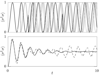
Figure 2: Quantum jumps in a driven two-level atom. Top: evolution of the excited-state probability for a single atom (quantum trajectory) with jumps to the ground state, corresponding to a detected photon. Four other trajectories are included to illustrate the dephasing due to the random nature of the jumps. Bottom: ensemble-averaged excited-state probability computed from the master equation (solid line), an average of 20 trajectories (dashed line), and an average of 2000 trajectories (dotted line). Time is measured in units of $2\pi/\Omega$ [see Eq. (169)], and the decay rate is $\Gamma=0.1$ in the same units.

X.3 Imaged Detection of Fluorescence

X.3.1 Center-of-Mass Dynamics

Now we want to consider how the evolution of the atomic internal state influences the atomic center-of-mass motion. To account for the external atomic motion, we use the center-of-mass Hamiltonian

$$H_{\mathrm{\scriptscriptstyle CM}}=\frac{p^{2}}{2m}+V(x)$$ (139)

in addition to the internal atomic Hamiltonian $H_{\mathrm{\scriptscriptstyle A}}$. We also need to explicitly include the spatial dependence of the field by letting

$$g_{\mathbf{k}}\longrightarrow g_{\mathbf{k}}e^{i\mathbf{k}\cdot\mathbf{r}}$$ (140)

in the interaction Hamiltonian (105). In the weak-excitation limit, we can take $\mathbf{k}$ to have the value $\mathbf{k}_{\mathrm{\scriptscriptstyle L}}$ of an externally applied probe field (the emitted photons are elastically scattered from the incident field).

To include the center of mass in the atomic state, we can explicitly write the state in terms of momentum-dependent coefficients as

$$|{\psi}\rangle=\int d\mathbf{p}\,\psi_{\mathrm{e}}(\mathbf{p})|{\mathbf{p},\mathrm{e}}\rangle+\sum_{\mathbf{k},\zeta}\psi_{\mathbf{k},\zeta}(\mathbf{p})|{\mathbf{p},\mathrm{g},1_{\mathbf{k},\zeta}}\rangle.$$ (141)

Notice that the new interaction Hamiltonian

$$H_{\mathrm{\scriptscriptstyle AF}}=\sum_{\mathbf{k},\zeta}\hbar\left(g_{\mathbf{k},\zeta}a_{\mathbf{k},\zeta}\sigma^{\dagger}e^{i\mathbf{k}\cdot\mathbf{r}}+g^{*}_{\mathbf{k},\zeta}a^{\dagger}_{\mathbf{k},\zeta}\sigma e^{-i\mathbf{k}\cdot\mathbf{r}}\right)$$ (142)

couples the state $|{\mathbf{p},\mathrm{e}}\rangle$ to the states $|{\mathbf{p}-\hbar\mathbf{k},\mathrm{g},1_{\mathbf{k},\zeta}}\rangle$ (in the momentum basis), giving rise to the atomic momentum recoil from spontaneous emission. (The additional recoil due to the absorption of the photon comes about by examining the coupling to the driving field.) The derivation of the last section carries through here with the replacement

$$\sigma\longrightarrow\sigma e^{-i\mathbf{k}_{\mathrm{\scriptscriptstyle L}}\cdot\mathbf{r}}.$$ (143)

Summing over all possible emission directions, the unconditioned master equation (128) becomes

$$\partial_{t}\rho=-\,\frac{i}{\hbar}[H_{\mathrm{\scriptscriptstyle A}}+H_{\mathrm{\scriptscriptstyle CM}},\rho]+\Gamma\int d\Omega\,f(\theta,\phi)\,\mathcal{D}\!\left[\sigma e^{-i\mathbf{k}_{\mathrm{\scriptscriptstyle L}}\cdot\mathbf{r}}\right]\rho,$$ (144)

where $f(\theta,\phi)$ is the normalized classical angular distribution for the radiated light, which here represents the angular probability distribution for the emitted photons.

Applying the same reasoning here as for the quantum-jump master equation (135), we obtain

$$\begin{array}[]{rcl}d\rho&{}={}&\displaystyle-\,\frac{i}{\hbar}[H_{\mathrm{\scriptscriptstyle A}}+H_{\mathrm{\scriptscriptstyle CM}},\rho]dt+\frac{\Gamma}{2}\left[\!\left\langle{\sigma^{\dagger}\sigma}\right\rangle-\sigma^{\dagger}\sigma,\rho\right]_{+}dt\\ &&\displaystyle{}+\int d\Omega\left(\frac{\sigma e^{-i\mathbf{k}\cdot\mathbf{r}}\rho\sigma^{\dagger}e^{i\mathbf{k}\cdot\mathbf{r}}}{\!\left\langle{\sigma^{\dagger}\sigma}\right\rangle}-\rho\right)\frac{dN(\theta,\phi)}{d\Omega},\end{array}$$ (145)

where

$$\left\langle\!\left\langle{\frac{dN(\theta,\phi)}{d\Omega}}\right\rangle\!\right\rangle=\Gamma\!\left\langle{\sigma^{\dagger}\sigma}\right\rangle f(\theta,\phi)\,dt$$ (146)

as before. We can simplify this equation by carrying out the angular integral, defining $dN$ to be one whenever $\max[dN(\theta,\phi)]=1$. The result is

$$\begin{array}[]{rcl}d\rho&{}={}&\displaystyle-\,\frac{i}{\hbar}[H_{\mathrm{\scriptscriptstyle A}}+H_{\mathrm{\scriptscriptstyle CM}},\rho]dt+\frac{\Gamma}{2}\left[\!\left\langle{\sigma^{\dagger}\sigma}\right\rangle-\sigma^{\dagger}\sigma,\rho\right]_{+}dt\\ &&\displaystyle{}+\left(\frac{\sigma e^{-i\mathbf{k}_{\mathrm{\scriptscriptstyle L}}\cdot\mathbf{r}}\rho\sigma^{\dagger}e^{i\mathbf{k}\cdot\mathbf{r}}}{\!\left\langle{\sigma^{\dagger}\sigma}\right\rangle}-\rho\right)dN\end{array}$$ (147)

with

$$\left\langle\!\left\langle{dN}\right\rangle\!\right\rangle=\Gamma\!\left\langle{\sigma^{\dagger}\sigma}\right\rangle dt$$ (148)

as before. The angles $\theta$ and $\phi$ are then stochastic variables with probability density $f(\theta,\phi)\sin\theta$.

X.3.2 Imaging

The above master equation (145) is for an angle-resolving detector. What we see is that angle-resolved detection keeps explicit track of the atomic momentum kicks due to spontaneous emission. An imaging detector, on the other hand, gives up resolution of the direction of the emitted photon wave vector $\mathbf{k}$, thus obtaining instead some position information about the atom. An imaging system operates by summing fields from many directions together and then detecting the resulting interference pattern. The procedure for obtaining the measurement operators for the imaging system is as follows Holland et al. (1996); Greenwood et al. (1997). Notice that we can regard the master equation (145) as a normal jump process of the form (135), with measurement operators

$$\sigma(\theta,\phi)=\sqrt{f(\theta,\phi)}\,\sigma e^{ik_{\mathrm{\scriptscriptstyle L}}z\cos\theta},$$ (149)

where we sum over all possible emission angles. In writing down this operator, we are specializing to one-dimensional motion along the $z$-axis ($x=y=0$), so we only require the $z$-component $k\cos\theta$ of $\mathbf{k}$. This operator ranges from $-1$ to $1$ in $\cos\theta$ and from $0$ to $2\pi$ in $\phi$. Thus, we can write down Fourier coefficients, since these functions are defined on a bounded domain, with two indices $\alpha$ and $\beta$:

$$\tilde{\sigma}_{\alpha\beta}=\frac{\sigma}{\sqrt{4\pi}}\int_{0}^{2\pi}d\phi\int_{-1}^{1}d(\cos\theta)\,\sqrt{f(\theta,\phi)}\,e^{ik_{\mathrm{\scriptscriptstyle L}}z\cos\theta}e^{-i\alpha\pi\cos\theta}e^{-i\beta\phi}.$$ (150)

If we consider an atom whose radiation pattern is axially symmetric, then performing the $\phi$ integral amounts to letting $f(\theta,\phi)\longrightarrow f(\theta)/2\pi$, since the integral is nonzero only for $\beta=0$. Carrying this out and suppressing the $\beta$ dependence,

$$\tilde{\sigma}_{\alpha}=\frac{\sigma}{\sqrt{2}}\int_{-1}^{1}d(\cos\theta)\,\sqrt{f(\theta)}\,e^{ik_{\mathrm{\scriptscriptstyle L}}(z-\alpha\lambda/2)\cos\theta}.$$ (151)

Notice that with the normalization convention for the Fourier coefficients here,

$$\int d\Omega\,\sigma^{\dagger}(\theta,\phi)\sigma(\theta,\phi)=\sum_{\alpha}\tilde{\sigma}^{\dagger}_{\alpha}\tilde{\sigma}_{\alpha},$$ (152)

so that the set of measurement operators is complete and properly normalized in either basis.

Notice that the $\tilde{\sigma}_{\alpha}$ operators contain localized functions of the position $z$, and thus correspond to position measurements. For example, a radiating atomic dipole oriented along the $z$-axis has

$$f(\theta)=\frac{3}{4}\sin^{2}\theta,$$ (153)

which gives measurement operators of the form

$$\tilde{\sigma}_{\alpha}=\sigma\sqrt{\frac{3\pi^{2}}{8}}\frac{J_{1}(k_{\mathrm{\scriptscriptstyle L}}z_{\alpha})}{k_{\mathrm{\scriptscriptstyle L}}z_{\alpha}},$$ (154)

where $z_{\alpha}:=z-\alpha\lambda/2$, and $J_{1}(x)$ is an ordinary Bessel function. Notice also that the set of possible measurement values is not continuous, but rather is discretely spaced by $\lambda/2$.

X.3.3 Gaussian Aperture

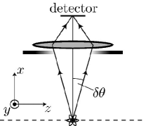
Figure 3: Basic setup for imaging resonance fluorescence from a single atom as a continuous position measurement. Light scattered from a probe laser (not shown) is collected by a Gaussian aperture of angular half-width $\delta\theta$ and focused by a lens on a position-sensitive detector, such as a photodiode array. The atom is constrained to move along the $z$-axis.

For the ideal imaging system we have considered here, the aperture extends over the full $4\pi$ solid angle (requiring, for example, arbitrarily large lenses on either side of the atom), though in practice it is rare to come anywhere close to this extreme. Thus, we will include the effects of an aperture that only allows the imaging system to detect radiated light within a limited solid angle (Fig. 3). For mathematical convenience, we will choose an aperture with a Gaussian spatial profile. We consider the above case of motion along the $z$-axis, with the atomic dipole oriented along the $z$-axis. Then photons going into any azimuthal angle $\phi$ are equivalent as far as providing position information about the atom, since the form of $\sigma(\theta,\phi)$ is independent of $\phi$. Thus, it suffices to consider only the $\theta$ dependence of the aperture, as any $\phi$ dependence contributes only by reducing the effective detection efficiency of the photodetector. Intuitively, one expects a camera imaging system to be most effective when oriented normal to the $z$-axis, so we choose the aperture to be centered about $\theta=\pi/2$. We thus take the intensity transmission function of the aperture to be

$$T(\theta)=\exp\left[-\,\frac{2(\theta-\pi/2)^{2}}{(\delta\theta)^{2}}\right].$$ (155)

The generalization of Eq. (151) to this case is

$$\tilde{\sigma}_{\alpha}=\frac{\sigma}{\sqrt{2}}\int_{-1}^{1}d(\cos\theta)\,\sqrt{T(\theta)f(\theta)}\,e^{ik_{\mathrm{\scriptscriptstyle L}}(z-\alpha\lambda/2)\cos\theta}.$$ (156)

If $\delta\theta$ is small, then the integrand is only appreciable for $\theta$ near $\pi/2$ due to the Gaussian factor. Recentering the integrand, making the small-angle approximation in the rest of the integrand, and extending the limits of integration, we find

$$\begin{array}[]{rcl}\tilde{\sigma}_{\alpha}&{}={}&\displaystyle\sigma\sqrt{\frac{3}{8}}\int_{-\pi/2}^{\pi/2}\!\!\!\!\!d\theta\,\cos^{2}\theta\,e^{-ik_{\mathrm{\scriptscriptstyle L}}(z-\alpha\lambda/2)\sin\theta}\exp\left[-\,\frac{\theta^{2}}{(\delta\theta)^{2}}\right]\\ &{}\approx{}&\displaystyle\sigma\sqrt{\frac{3}{8}}\int_{-\infty}^{\infty}\!\!\!d\theta\,e^{-ik_{\mathrm{\scriptscriptstyle L}}(z-\alpha\lambda/2)\theta}\exp\left[-\,\frac{\theta^{2}}{(\delta\theta)^{2}}\right]\\ &{}={}&\displaystyle\sigma\sqrt{\frac{3\pi}{8}}\delta\theta\,\exp\left[-\left(\frac{k_{\mathrm{\scriptscriptstyle L}}\,\delta\theta}{2}\right)^{2}\,\left(z-\frac{\alpha\lambda}{2}\right)^{2}\right].\end{array}$$ (157)

Thus, the measurement operator in this case is actually Gaussian. We can write the fraction of photons transmitted by the aperture as an efficiency

$$\eta_{\theta}:=\int_{-1}^{1}d(\cos\theta)\,T(\theta)f(\theta)\approx\frac{3}{4}\sqrt{\frac{\pi}{2}}\,\delta\theta$$ (158)

in the same regime of small $\delta\theta$. Then the Gaussian measurement operators $\tilde{\sigma}_{\alpha}$ satisfy

$$\sum_{\alpha}\tilde{\sigma}_{\alpha}^{\dagger}\tilde{\sigma}_{\alpha}=\eta_{\theta}\sigma^{\dagger}\sigma.$$ (159)

This normalization is sensible, although as we will see later, $\eta_{\theta}$ turns out not to be the actual measurement efficiency.

X.3.4 Spatial Continuum Approximation

If an atom is initially completely delocalized, after one photon is detected and the collapse operator $\tilde{\sigma}_{\alpha}$ applies, the atom is reduced to a width of order

$$\delta\alpha=\frac{1}{k_{\mathrm{\scriptscriptstyle L}}\,\delta\theta}=\frac{\lambda}{2\pi\,\delta\theta}.$$ (160)

Since this is much larger than the spacing

$$\Delta\alpha=\frac{\pi}{k_{\mathrm{\scriptscriptstyle L}}}=\frac{\lambda}{2},$$ (161)

it is effectively impossible to “see” the discreteness of the measurement record, and it is a good approximation to replace the set of measurement operators with a set corresponding to a continuous range of possible measurement outcomes. Since in the limit of small spacing $\Delta x$, it is a good approximation to write an integral as a sum

$$\sum_{n}f(n\Delta x)\,\Delta x=\int dx\,f(x)$$ (162)

for an arbitrary function $f(x)$, we can make the formal identification

$$\tilde{\sigma}_{\alpha}\longrightarrow\frac{\tilde{\sigma}(\alpha)}{\sqrt{\Delta\alpha}}$$ (163)

to obtain the continuum limit of the position collapse operators. Thus, we have

$$\begin{array}[]{rcl}\tilde{\sigma}(\alpha)&{}={}&\displaystyle\int dz|{z}\rangle\langle{z}|\,\sigma\sqrt{\eta_{\theta}}\frac{1}{\sqrt{\sqrt{2\pi}\,\delta\alpha}}\exp\left[-\,\frac{\left(z-\alpha\right)^{2}}{4(\delta\alpha)^{2}}\right].\end{array}$$ (164)

We have inserted the identity here to make this expression a proper operator on the atomic center-of-mass state. Again, $\alpha$ is now a continuous index with dimensions of length, rather than an integer index.

Thus, from the form of Eq. (137), we can deduce the following form of the master equation for imaged photodetection through the Gaussian aperture:

$$\begin{array}[]{rcl}d\rho&{}={}&\displaystyle-\,\frac{i}{\hbar}[H_{\mathrm{\scriptscriptstyle A}}+H_{\mathrm{\scriptscriptstyle CM}},\rho]dt+\Gamma\int d\Omega\,\mathcal{D}[\sigma(\theta,\phi)]\rho\,dt\\ &&\displaystyle{}+\eta_{\theta}\Gamma\!\left\langle{\sigma^{\dagger}\sigma}\right\rangle\rho\,dt\\ &&\displaystyle{}-\Gamma\int d\Omega\,T(\theta)\,\sigma(\theta,\phi)\,\rho\,\sigma^{\dagger}(\theta,\phi)\,dt\\ &&\displaystyle{}+\left[\frac{\tilde{\sigma}(\alpha)\,\rho\,\tilde{\sigma}^{\dagger}(\alpha)}{\!\left\langle{\tilde{\sigma}^{\dagger}(\alpha)\tilde{\sigma}(\alpha)}\right\rangle}-\rho\right]dN.\end{array}$$ (165)

Recalling the normalization

$$\int d\Omega\,T(\theta)\,\sigma^{\dagger}(\theta,\phi)\sigma(\theta,\phi)=\int d\alpha\,\tilde{\sigma}^{\dagger}(\alpha)\tilde{\sigma}(\alpha)=\eta_{\theta}\sigma^{\dagger}\sigma,$$ (166)

we have for the Poisson process

$$\left\langle\!\left\langle{dN}\right\rangle\!\right\rangle=\Gamma\,dt\int d\alpha\!\left\langle{\tilde{\sigma}^{\dagger}(\alpha)\tilde{\sigma}(\alpha)}\right\rangle=\eta_{\theta}\Gamma\!\left\langle{\sigma^{\dagger}\sigma}\right\rangle dt.$$ (167)

Again, $\alpha$ is a random real number corresponding to the result of the position measurement for a given spontaneous emission event. The probability density for $\alpha$ is

$$\begin{array}[]{rcl}P(\alpha)&{}={}&\displaystyle\frac{\!\left\langle{\tilde{\sigma}^{\dagger}(\alpha)\tilde{\sigma}(\alpha)}\right\rangle}{\eta_{\theta}\!\left\langle{\sigma^{\dagger}\sigma}\right\rangle}\\ &{}={}&\displaystyle\frac{1}{\!\left\langle{\sigma^{\dagger}\sigma}\right\rangle}\int dz\,|\psi_{\mathrm{e}}(z)|^{2}\frac{1}{\sqrt{2\pi}\,\delta\alpha}\exp\left[-\,\frac{(z-\alpha)^{2}}{2(\delta\alpha)^{2}}\right],\end{array}$$ (168)

that is, in the case of a localized atomic wave packet, a Gaussian probability density with variance $(\delta\alpha)^{2}$.

X.4 Adiabatic Approximation

So far, we have seen how the internal and external dynamics of the atom are intrinsically linked. Now we would like to focus on the external atomic dynamics. To do so, we will take advantage of the natural separation of time scales of the dynamics. The internal dynamics are damped at the spontaneous emission rate $\Gamma$, which is typically on the order of $\sim\!\!10^{7}\;\mathrm{s}^{-1}$. The external dynamics are typically much slower, corresponding to kHz or smaller oscillation frequencies for typical laser dipole traps. The adiabatic approximation assumes that the internal dynamics equilibrate rapidly compared to the external dynamics, and are thus always in a quasi-equilibrium state with respect to the external state.

X.4.1 Internal Quasi-Equilibrium

In treating the internal dynamics, we have noted that the atom decays, but not why it was excited in the first place. A resonant, driving (classical) laser field enters in the form Loudon (1983)

$$H_{\mathrm{\scriptscriptstyle D}}=\frac{\hbar\Omega}{2}\left(\sigma+\sigma^{\dagger}\right),$$ (169)

where the Rabi frequency $\Omega$ characterizes the strength of the laser–atom interaction. In writing down this interaction, we have implicitly made the standard unitary transformation to a rotating frame where $H_{\mathrm{\scriptscriptstyle A}}=0$. We have also assumed the driving field propagates along a normal to the $z$-axis, so we have not written any spatial dependence of the field in $H_{\mathrm{\scriptscriptstyle D}}$.

The usual unconditioned master equation with this interaction, but neglecting the external motion (that is equivalent to the usual, on-resonance optical Bloch equations) is

$$\partial_{t}\rho=-\,\frac{i}{\hbar}[H_{\mathrm{\scriptscriptstyle D}},\rho]+\Gamma\mathcal{D}[\sigma]\rho.$$ (170)

This equation implies that the expectation value of an operator $A$ evolves as

$$\partial_{t}\!\left\langle{A}\right\rangle=-\,\frac{i}{\hbar}\!\left\langle{[A,H_{\mathrm{\scriptscriptstyle D}}]}\right\rangle+\Gamma\!\left\langle{\sigma^{\dagger}A\sigma-\frac{1}{2}[\sigma^{\dagger}\sigma,A]_{+}}\right\rangle.$$ (171)

This gives the following equations of motion for the density-matrix elements:

$$\begin{array}[]{rcl}\partial_{t}\rho_{\mathrm{ee}}&{}={}&\displaystyle\partial_{t}\!\left\langle{\sigma^{\dagger}\sigma}\right\rangle=\frac{i\Omega}{2}\left(\!\left\langle{\sigma}\right\rangle-\!\left\langle{\sigma^{\dagger}}\right\rangle\right)-\Gamma\!\left\langle{\sigma^{\dagger}\sigma}\right\rangle,\\ \partial_{t}\rho_{\mathrm{eg}}&{}={}&\displaystyle\partial_{t}\!\left\langle{\sigma}\right\rangle=\frac{i\Omega}{2}\left(\!\left\langle{\sigma^{\dagger}\sigma}\right\rangle-\!\left\langle{\sigma\sigma^{\dagger}}\right\rangle\right)-\frac{\Gamma}{2}\!\left\langle{\sigma}\right\rangle.\end{array}$$ (172)

The remaining matrix elements are determined by $\rho_{\mathrm{ge}}=\rho_{\mathrm{eg}}^{*}$ and $\rho_{\mathrm{gg}}=\!\left\langle{\sigma\sigma^{\dagger}}\right\rangle=1-\,\!\left\langle{\sigma^{\dagger}\sigma}\right\rangle$. Setting the time derivatives to zero, we can solve these equations to obtain

$$\begin{array}[]{rcl}\!\left\langle{\sigma^{\dagger}\sigma}\right\rangle_{\mathrm{ss}}&{}={}&\displaystyle\frac{\Omega^{2}/\Gamma^{2}}{1+2\Omega^{2}/\Gamma^{2}},\\ \!\left\langle{\sigma}\right\rangle_{\mathrm{ss}}&{}={}&\displaystyle\frac{-i\Omega/\Gamma}{1+2\Omega^{2}/\Gamma^{2}},\end{array}$$ (173)

for the internal steady-state of the atom.

X.4.2 External Master Equation

To make the adiabatic approximation and eliminate the internal dynamics, we note that there is no effect on the external dynamics apart from the slow center-of-mass motion in the potential $V(x)$ and the collapses due to the detection events. When the internal timescales damp much more quickly than the external time scales, we can make the replacement

$$\!\left\langle{\sigma^{\dagger}\sigma}\right\rangle\longrightarrow\!\left\langle{\sigma^{\dagger}\sigma}\right\rangle_{\mathrm{ss}}$$ (174)

in the master equation (165). Also, in steady state, the internal equations of motion (172) give

$$\!\left\langle{\sigma^{\dagger}\sigma}\right\rangle=\frac{\Omega^{2}/\Gamma^{2}}{1+\Omega^{2}/\Gamma^{2}}\!\left\langle{\sigma\sigma^{\dagger}}\right\rangle,$$ (175)

so that the ground- and excited-state populations are proportional. When we also account for the atomic spatial dependence, this argument applies at each position $z$, so that we can write

$$|\psi_{\mathrm{e}}(z)|^{2}=\frac{\Omega^{2}/\Gamma^{2}}{1+\Omega^{2}/\Gamma^{2}}|\psi_{\mathrm{g}}(z)|^{2},$$ (176)

where we are using the general decomposition

$$\langle z|\psi\rangle=\psi_{\mathrm{e}}(z)|{\mathrm{e}}\rangle+\psi_{\mathrm{g}}(z)|{\mathrm{g}}\rangle$$ (177)

for the atomic state vector. Thus, the spatial profile of the atom is independent of its internal state, so we need not assign multiple wave functions $\psi_{\mathrm{g}}(z)$ and $\psi_{\mathrm{e}}(z)$ to different internal states of the atom.

Furthermore, we will take a partial trace over the internal degrees of freedom by defining the external density operator

$$\rho_{\mathrm{ext}}:=\!\left\langle{\mathrm{e}|\rho|\mathrm{e}}\right\rangle+\!\left\langle{\mathrm{g}|\rho|\mathrm{g}}\right\rangle.$$ (178)

The result of applying the same partial trace on the master equation is

$$\begin{array}[]{rcl}d\rho_{\mathrm{ext}}&{}={}&\displaystyle-\,\frac{i}{\hbar}[H_{\mathrm{\scriptscriptstyle CM}},\rho_{\mathrm{ext}}]dt\\ &&\displaystyle{}+\gamma\int d\Omega\,[1-T(\theta)]\,f(\theta,\phi)\,\mathcal{D}[e^{-ik_{\mathrm{\scriptscriptstyle L}}z\cos\theta}]\rho_{\mathrm{ext}}\,dt\\ &&\displaystyle{}+\left[\frac{A(\alpha)\,\rho_{\mathrm{ext}}\,A^{\dagger}(\alpha)}{\!\left\langle{A^{\dagger}(\alpha)A(\alpha)}\right\rangle}-\rho_{\mathrm{ext}}\right]dN,\end{array}$$ (179)

where

$$\begin{array}[]{rcl}\left\langle\!\left\langle{dN}\right\rangle\!\right\rangle&{}={}&\displaystyle\eta_{\theta}\gamma\,dt\\ \tilde{\sigma}(\alpha)&{}=:{}&\sigma A(\alpha)\\ \gamma&{}:={}&\Gamma\!\left\langle{\sigma^{\dagger}\sigma}\right\rangle.\end{array}$$ (180)

The form (179) follows from the fact that the density operator $\rho$ factorizes into external and internal parts, as we saw in Eq. (177). Also, Eq. (168) becomes

$$\begin{array}[]{rcl}P(\alpha)&{}={}&\displaystyle\int dz\,|\psi(z)|^{2}\frac{1}{\sqrt{2\pi}\,\delta\alpha}\exp\left[-\,\frac{(z-\alpha)^{2}}{2(\delta\alpha)^{2}}\right],\end{array}$$ (181)

where $\psi(z)$ is the effective state-independent wave function for the atom. When the external state is not pure, we simply make the substitution $|\psi(z)|^{2}\longrightarrow\langle{z}|\rho_{\mathrm{ext}}|{z}\rangle$ in Eq. (181) to handle this.

Now we have what we want: a master equation for the atomic center-of-mass state that exhibits localizing collapses due to a physical measurement process. What we essentially have is continuous evolution, with the end of each interval of mean length $(\eta_{\theta}\gamma)^{-1}$ punctuated by a POVM-type reduction of the form $\rho\longrightarrow A(\alpha)\rho A^{\dagger}(\alpha)$. But note that here there is extra disturbance for the amount of information we gain, because the aperture only picks up a fraction of the available information. We will return to this point shortly.

X.5 White-Noise Limit

We now have a POVM with a form similar to Eq. (22), but we still have a quantum-jump master equation for a position measurement that does not look like Eq. (32). However, we can note that the Gaussian form of the collapse operator $A(\alpha)$ is applied to the state after every time interval of average length $\Delta t=(\eta_{\theta}\gamma)^{-1}$. In the regime of slow atomic center-of-mass motion, the collapses come quickly compared to the motion. Then it is a good approximation to take the formal limit $\Delta t\longrightarrow 0$, while keeping the rate of information gain constant. (Note that the same result arises in homodyne detection, where the emitted light interferes with a strong phase-reference field, without any coarse-graining approximation.)

X.5.1 Quantum-State Diffusion

Comparing Eq. (181) with Eq. (24), we see that they are the same if we identify

$$4k\Delta t=\frac{1}{2(\delta\alpha)^{2}}.$$ (182)

Note that $k$ here refers to the measurement strength, not the wave number $k_{\mathrm{\scriptscriptstyle L}}$ of the scattered light. Solving for the measurement strength,

$$k=\frac{\eta_{\theta}\gamma}{8(\delta\alpha)^{2}}=\frac{\pi^{2}\eta_{\theta}\gamma(\delta\theta)^{2}}{2\lambda^{2}}.$$ (183)

Repeating the procedure of Section IV, we can take the limit $\Delta t\longrightarrow 0$ with $k$ fixed. The resulting master equation, in “quantum-state diffusion” form, is

$$\begin{array}[]{rcl}d\rho_{\mathrm{ext}}&{}={}&\displaystyle-\,\frac{i}{\hbar}[H_{\mathrm{\scriptscriptstyle CM}},\rho_{\mathrm{ext}}]dt\\ &&\displaystyle{}+\gamma\int d\Omega\,[1-T(\theta)]\,f(\theta,\phi)\,\mathcal{D}[e^{-ik_{\mathrm{\scriptscriptstyle L}}z\cos\theta}]\rho_{\mathrm{ext}}\,dt\\ &&\displaystyle{}+2k\mathcal{D}[z]\rho_{\mathrm{ext}}\,dt{}+\sqrt{2\eta_{\phi}k}\mathcal{H}[z]\rho_{\mathrm{ext}}\,dW.\end{array}$$ (184)

The form here is the same as in Eq. (32), except for an extra “disturbance term” representing the undetected photons. We have also added an extra efficiency $\eta_{\phi}$ to model aperturing in the $\phi$ direction and other effects such as the intrinsic (quantum) efficiency of the imaging detector.

X.5.2 Diffusion Rates

To simplify the master equation (184), we will analyze the diffusion rates due to the second and third terms (proportional to $\gamma$ and $k$, respectively). From the analysis of Eqs. (97), recall that the term $2k\mathcal{D}[z]\rho_{\mathrm{ext}}\,dt$ causes diffusion in momentum at the rate

$$D_{k}=2\hbar^{2}k=\frac{\eta_{\theta}}{4}\gamma\hbar^{2}k_{\mathrm{\scriptscriptstyle L}}^{2}(\delta\theta)^{2}.$$ (185)

This is the disturbance corresponding to the information gain. The relation $k=D_{k}/(2\hbar^{2})$ will be useful below.

We can compute the total diffusion rate due to the spontaneously emitted photons as follows. Each photon emission causes a momentum kick of magnitude $\hbar k_{\mathrm{\scriptscriptstyle L}}\cos\theta$, and the spontaneous emission rate is $\gamma$. Averaging over the angular photon distribution, the diffusion rate becomes

$$D_{\mathrm{\scriptscriptstyle SE}}=\gamma\hbar^{2}k_{\mathrm{\scriptscriptstyle L}}^{2}\int d\Omega\,f(\theta,\phi)\cos^{2}\theta=\frac{\gamma\hbar^{2}k_{\mathrm{\scriptscriptstyle L}}^{2}}{5}.$$ (186)

On the other hand, the diffusion rate due only to the detected photons is

$$\begin{array}[]{rcl}D_{\theta}&{}={}&\displaystyle\gamma\hbar^{2}k_{\mathrm{\scriptscriptstyle L}}^{2}\int d\Omega\,T(\theta)\,f(\theta,\phi)\cos^{2}\theta\\ &{}={}&\displaystyle\gamma\hbar^{2}k_{\mathrm{\scriptscriptstyle L}}^{2}\frac{3}{4}\int_{0}^{\pi}d\theta\,\sin^{3}\theta\,\cos^{2}\theta\exp\left[-\,\frac{2(\theta-\pi/2)^{2}}{(\delta\theta)^{2}}\right]\\ &{}\approx{}&\displaystyle\frac{\eta_{\theta}}{4}\gamma\hbar^{2}k_{\mathrm{\scriptscriptstyle L}}^{2}(\delta\theta)^{2},\end{array}$$ (187)

where we used the fact that $\delta\theta$ is small. This is precisely the same rate as $D_{k}$, since they are two different representations of the same physical process.

We see now that the second and third terms of Eq. (184) have the same effect of momentum diffusion, but at different rates. We can formally combine them to obtain

$$\begin{array}[]{rcl}d\rho_{\mathrm{ext}}&{}={}&\displaystyle-\,\frac{i}{\hbar}[H_{\mathrm{\scriptscriptstyle CM}},\rho_{\mathrm{ext}}]dt\\ &&\displaystyle{}+2k_{\mathrm{eff}}\mathcal{D}[z]\rho_{\mathrm{ext}}\,dt{}+\sqrt{2\eta_{\mathrm{eff}}k_{\mathrm{eff}}}\mathcal{H}[z]\rho_{\mathrm{ext}}\,dW,\end{array}$$ (188)

where the effective measurement strength is

$$k_{\mathrm{eff}}=\frac{D_{\mathrm{\scriptscriptstyle SE}}}{2\hbar^{2}}=\frac{\gamma k_{\mathrm{\scriptscriptstyle L}}^{2}}{10},$$ (189)

and the effective measurement efficiency is

$$\eta_{\mathrm{eff}}=\frac{\eta_{\phi}k}{k_{\mathrm{eff}}}=\frac{5}{4}\eta_{\phi}\eta_{\theta}(\delta\theta)^{2}.$$ (190)

Notice that since $\delta\theta$ is assumed small, the apparent efficiency $\eta_{\mathrm{eff}}$ derived from comparing the information rate to the disturbance rate, is much smaller than the photon-detection efficiency of $\eta_{\phi}\eta_{\theta}$. Evidently, the photons radiated near $\theta=\pi/2$ are much less effective compared to the photons radiated near $\theta=0$ or $\pi$. This result is counterintuitive when considering typical imaging setups as we have considered here, but suggests that other ways of processing the radiated photons (e.g., measuring the phase of photons radiated closer to the $z$-axis) are more effective than camera-like imaging.

XI Conclusion

We have presented what we hope is a readily accessible introduction to continuous measurements in quantum systems. If you have read and digested most of the above, you should have a good basic understanding of how to treat such measurements and manipulate the equations that describe them. There is now a considerable literature discussing such measurements in a variety of systems, and here we give a brief overview of this literature so as to provide a pointer to further reading. We have already mentioned that continuous measurement has many applications in areas such as feedback control and metrology, and references on these topics have been given in the introduction. The early pioneering work on continuous measurement may be found in Refs. Srinivas and Davies (1981); Barchielli et al. (1982); Gisin (1984); Barchielli and Lupieri (1985); Diosi (1986a); Belavkin (1987); Diosi (1986b); Belavkin (1989). Derivations of continuous measurements driven by Gaussian noise in quantum-optical systems are given in Refs. Carmichael et al. (1989); Wiseman and Milburn (1993b); Doherty and Jacobs (1999), and further applications in quantum optics may be found in Refs. Wiseman (1993); Carmichael (1993); Garraway and Knight (1994); Wiseman (1995, 1996b); Plenio and Knight (1998); Wiseman (1996a). Derivations and applications of stochastic Schrödinger equations with jump (Poisson) processes—developed originally in quantum optics as a tool for the simulation of master equations using the “Monte Carlo” method, as in Section X.2—may be found in Zoller et al. (1987); Hegerfeldt and Wilser (1991); Holland et al. (1991); Dalibard et al. (1992); Gardiner et al. (1992); Plenio (1994); Hegerfeldt and Plenio (1996); Garraway and Knight (1994); Holland et al. (1996); Plenio and Knight (1998). A treatment of continuous measurement in a solid-state system is given in Korotkov (2001), and further applications in these systems may be found in Goan and Milburn (2001); Hopkins et al. (2003); Brun and Goan (2003); Santamore et al. (2004); Ruskov et al. (2005); Sarovar et al. (2005); Jordan and Korotkov (2006). Last, but not least, if the reader is interested in treatments of quantum continuous measurements using the rigorous mathematical language of filtering theory, these may be found in Refs. Bouten et al. (2006); Belavkin (1993, 1994, 1987). Other rigorous treatments are given in Refs. Barchielli and Lupieri (1985); Barchielli (1993).

XII Acknowledgments

The authors would like to thank Tanmoy Bhattacharya, Michael Raymer, Elizabeth Schoene, and Jeremy Thorn for insightful comments and corrections. D.A.S. acknowledges support from the National Science Foundation, and K.J. acknowledges support from the Hearne Institute for Theoretical Physics, the National Security Agency, the Army Research Office, and the Disruptive Technologies Office.

Kurt Jacobs is an Assistant Professor of Physics at the University of Massachusetts at Boston. He completed a master’s degree in physics with Dan Walls at Auckland University in 1995, and a Ph.D. with Peter Knight at Imperial College, London, in 1998. During his time at Auckland he was introduced to classical continuous measurement theory by Sze Tan, and was exposed to the recently developed field of quantum continuous measurement particularly in interactions with Howard Wiseman who was then a postdoc at Auckland. He continued to work on this subject during his Ph.D., and then joined Los Alamos National Laboratory where he worked with Salman Habib on problems in quantum feedback control and the quantum-to-classical transition. His work currently focuses on these two areas, including applications of continuous measurement and control in atom optics and quantum-nano-electro mechanics.

Daniel Steck is an Assistant Professor of Physics at the University of Oregon. He performed his Ph.D. work, involving experiments in quantum chaos and transport, with Mark Raizen at the University of Texas at Austin. He was then a postdoctoral fellow at Los Alamos National Laboratory with Salman Habib, working on the theory of quantum measurement and feedback control. His work now focuses on the study of continuous quantum measurements and the transition between quantum and classical dynamics in ultracold-atom experiments.

References

- Belavkin (1987) V. P. Belavkin, in Information, Complexity and Control in Quantum Physics, edited by A. Blaquiere, S. Diner, and G. Lochak (Springer-Verlag, New York, 1987).
- Bushev et al. (2006) P. Bushev, D. Rotter, A. Wilson, F. Dubin, C. Becher, J. Eschner, R. Blatt, V. Steixner, P. Rabl, and P. Zoller, Phys. Rev. Lett. 96, 043003 (2006).
- Combes and Jacobs (2006) J. Combes and K. Jacobs, Phys. Rev. Lett. 96, 010504 (2006).
- D’Helon and James (2006) C. D’Helon and M. R. James, Phys. Rev. A 73, 053803 (2006).
- Doherty and Jacobs (1999) A. C. Doherty and K. Jacobs, Phys. Rev. A 60, 2700 (1999).
- Hopkins et al. (2003) A. Hopkins, K. Jacobs, S. Habib, and K. Schwab, Phys. Rev. B 68, 235328 (2003).
- Rabl et al. (2005) P. Rabl, V. Steixner, and P. Zoller, Eprint: quant-ph/0506185 (2005).
- Steck et al. (2004) D. Steck, K. Jacobs, H. Mabuchi, T. Bhattacharya, and S. Habib, Phys. Rev. Lett. 92, 223004 (2004).
- Steck et al. (2006) D. Steck, K. Jacobs, H. Mabuchi, S. Habib, and T. Bhattacharya, Phys. Rev. A 74, 012322 (2006).
- Steixner et al. (2005) V. Steixner, P. Rabl, and P. Zoller, Eprint: quant-ph/0506187 (2005).
- Wiseman and Doherty (2005) H. M. Wiseman and A. C. Doherty, Phys. Rev. Lett. 94, 070405 (2005).
- Berry and Wiseman (2002) D. W. Berry and H. M. Wiseman, Phys. Rev. A 65, 043803 (2002).
- Geremia et al. (2005) J. Geremia, J. K. Stockton, and H. Mabuchi, Phys. Rev. Lett. 94, 203002 (2005).
- Pope et al. (2004) D. T. Pope, H. M. Wiseman, and N. K. Langford, Phys. Rev. A 70, 043812 (2004).
- Stockton et al. (2004) J. K. Stockton, J. M. Geremia, A. C. Doherty, and H. Mabuchi, Phys. Rev. A 69, 032109 (2004).
- Wiseman (1995) H. M. Wiseman, Phys. Rev. Lett. 75, 4587 (1995).
- Dolinar (1973) S. Dolinar, Tech. Rep. 111, Research Laboratory of Electronics (MIT, Cambridge, 1973).
- Geremia (2004) J. M. Geremia, Phys. Rev. A 70, 062303 (2004).
- Jacobs (2007) K. Jacobs, Quant. Information Comp. 7, 127 (2007).
- Ahn et al. (2002) C. Ahn, A. C. Doherty, and A. J. Landahl, Phys. Rev. A 65, 042301 (2002).
- Sarovar et al. (2004) M. Sarovar, C. Ahn, K. Jacobs, and G. J. Milburn, Phys. Rev. A 69, 052324 (2004).
- van Handel and Mabuchi (2006) R. van Handel and H. Mabuchi, Eprint: quant-ph/0511221 (2006).
- Bhattacharya et al. (2000) T. Bhattacharya, S. Habib, and K. Jacobs, Phys. Rev. Lett. 85, 4852 (2000).
- Bhattacharya et al. (2003) T. Bhattacharya, S. Habib, and K. Jacobs, Phys. Rev. A 67, 042103 (2003).
- Everitt et al. (2005) M. J. Everitt, T. D. Clark, P. B. Stiffell, J. F. Ralph, A. Bulsara, and C. Harland, New J. Phys. 7, 64 (2005).
- Ghose et al. (2004) S. Ghose, P. Alsing, I. Deutsch, T. Bhattacharya, and S. Habib, Phys. Rev. A 69, 052116 (2004).
- Ghose et al. (2005) S. Ghose, P. M. Alsing, B. C. Sanders, and I. H. Deutsch, Phys. Rev. A 72, 014102 (2005).
- Habib et al. (2002) S. Habib, K. Jacobs, H. Mabuchi, R. Ryne, K. Shizume, and B. Sundaram, Phys. Rev. Lett. 88, 040402 (2002).
- Habib et al. (2006) S. Habib, K. Jacobs, and K. Shizume, Phys. Rev. Lett. 96, 010403 (2006).
- Brun (2002) T. A. Brun, Am. J. Phys. 70, 719 (2002).
- Braginsky et al. (1995) V. B. Braginsky, F. Y. Khalili, and K. S. Thorne, Quantum Measurement (Cambridge, 1995).
- Wiseman (1996a) H. M. Wiseman, Quant. Semiclass. Opt. 8, 205 (1996a).
- Carmichael (1993) H. Carmichael, An Open Systems Approach to Quantum Optics (Springer-Verlag, Berlin, 1993).
- Nielsen and Chuang (2000) M. A. Nielsen and I. L. Chuang, Quantum Computation and Quantum Information (Cambridge University Press, 2000).
- Schumacher (1996) B. Schumacher, Phys. Rev. A 54, 2614 (1996).
- Fuchs and Jacobs (2001) C. A. Fuchs and K. Jacobs, Phys. Rev. A 63, 062305 (2001).
- Kloeden and Platen (1992) P. E. Kloeden and E. Platen, Numerical Solution of Stochastic Differential Equations (Springer, Berlin, 1992).
- Caves and Milburn (1987) C. M. Caves and J. G. Milburn, Phys. Rev. A 36, 5543 (1987).
- Gardiner (1985) C. W. Gardiner, Handbook of Stochastic Methods (Springer, 1985).
- Gillespie (1996) D. T. Gillespie, Am. J. Phys. 64, 225 (1996).
- Jacobs and Knight (1998) K. Jacobs and P. L. Knight, Phys. Rev. A 57, 2301 (1998).
- Barchielli (1993) A. Barchielli, Int. J. Theor. Phys. 32, 2221 (1993).
- Dziarmaga et al. (2004) J. Dziarmaga, D. A. R. Dalvit, and W. H. Zurek, Phys. Rev. A 69, 022109 (2004).
- Wiseman and Milburn (1993a) H. M. Wiseman and G. J. Milburn, Phys. Rev. A 47, 642 (1993a).
- Adler (2000) S. L. Adler, Phys. Lett. A 265, 58 (2000).
- Wiseman and Diosi (2001) H. M. Wiseman and L. Diosi, Chem. Phys. 91, 268 (2001).
- Lindblad (1976) G. Lindblad, Comm. Math. Phys. 48, 199 (1976).
- Habib (2004) S. Habib, Eprint: quant-ph/0406011 (2004).
- Landauer (1993) R. Landauer, Physica A 194, 551 (1993).
- Milonni (1994) P. W. Milonni, The Quantum Vacuum (Academic Press, 1994).
- Scully and Zubairy (1997) M. O. Scully and M. S. Zubairy, Quantum Optics (Cambridge, 1997).
- Weisskopf and Wigner (1930) V. Weisskopf and E. Wigner, Z. Phys. 63, 54 (1930).
- Greenwood et al. (1997) W. Greenwood, P. Pax, and P. Meystre, Phys. Rev. A 56, 2109 (1997).
- Holland et al. (1996) M. Holland, S. Marksteiner, P. Marte, and P. Zoller, Phys. Rev. Lett. 76, 3683 (1996).
- Loudon (1983) R. Loudon, The Quantum Theory of Light (Oxford University Press, Oxford, 1983), 2nd ed.
- Barchielli et al. (1982) A. Barchielli, L. Lanz, and G. M. Prosperi, Nuovo Cimento B 72, 79 (1982).
- Barchielli and Lupieri (1985) A. Barchielli and G. Lupieri, J. Math. Phys. 26, 2222 (1985).
- Belavkin (1989) V. P. Belavkin, Phys. Lett. A 140, 355 (1989).
- Diosi (1986a) L. Diosi, Phys. Lett. A 114, 451 (1986a).
- Diosi (1986b) L. Diosi, Phys. Lett. A 129, 419 (1986b).
- Gisin (1984) N. Gisin, Phys. Rev. Lett. 52, 1657 (1984).
- Srinivas and Davies (1981) M. D. Srinivas and E. B. Davies, Optica Acta 28, 981 (1981).
- Carmichael et al. (1989) H. J. Carmichael, S. Singh, R. Vyas, and P. R. Rice, Phys. Rev. A 39, 1200 (1989).
- Wiseman and Milburn (1993b) H. M. Wiseman and G. J. Milburn, Phys. Rev. A 47, 642 (1993b).
- Garraway and Knight (1994) B. M. Garraway and P. L. Knight, Phys. Rev. A 50, 2548 (1994).
- Plenio and Knight (1998) M. B. Plenio and P. L. Knight, Rev. Mod. Phys. 70, 101 (1998).
- Wiseman (1993) H. M. Wiseman, Phys. Rev. A 47, 5180 (1993).
- Wiseman (1996b) H. M. Wiseman, Quant. Semiclass. Opt. 8, 205 (1996b).
- Dalibard et al. (1992) J. Dalibard, Y. Castin, and K. Mølmer, Phys. Rev. Lett. 68, 580 (1992).
- Gardiner et al. (1992) C. W. Gardiner, A. S. Parkins, and P. Zoller, Phys. Rev. A 46, 4363 (1992).
- Hegerfeldt and Plenio (1996) G. C. Hegerfeldt and M. B. Plenio, Phys. Rev. A 53, 1164 (1996).
- Hegerfeldt and Wilser (1991) G. C. Hegerfeldt and T. S. Wilser, in Proceedings of the II International Wigner Symposium, edited by H. D. Doebner, W. Scherer, and F. Schroeck (World Scientific, Singapore, 1991), p. 104.
- Holland et al. (1991) M. J. Holland, D. F. Walls, and P. Zoller, Phys. Rev. Lett. 67, 1716 (1991).
- Plenio (1994) M. B. Plenio, Ph.D. thesis, University of Göttingen (1994).
- Zoller et al. (1987) P. Zoller, M. Marte, and D. F. Walls, Phys. Rev. A 35, 198 (1987).
- Korotkov (2001) A. N. Korotkov, Phys. Rev. B 63, 115403 (2001).
- Brun and Goan (2003) T. A. Brun and H.-S. Goan, Phys. Rev. A 68, 032301 (2003).
- Goan and Milburn (2001) H.-S. Goan and G. J. Milburn, Phys. Rev. B 64, 235307 (2001).
- Jordan and Korotkov (2006) A. N. Jordan and A. N. Korotkov, Phys. Rev. B 74, 085307 (2006).
- Ruskov et al. (2005) R. Ruskov, K. Schwab, and A. N. Korotkov, Phys. Rev. B 71, 235407 (2005).
- Santamore et al. (2004) D. H. Santamore, A. C. Doherty, and M. C. Cross, Phys. Rev. B 70, 144301 (2004).
- Sarovar et al. (2005) M. Sarovar, H.-S. Goan, T. P. Spiller, and G. J. Milburn, Phys. Rev. A 72, 062327 (2005).
- Belavkin (1993) V. P. Belavkin, Prob. Theory App. 38, 742 (1993).
- Belavkin (1994) V. P. Belavkin, Prob. Theory App. 39, 640 (1994).
- Bouten et al. (2006) L. Bouten, R. van Handel, and M. R. James, Eprint: math.PR/0606118 (2006).