Projective Ring Line Encompassing
Two-Qubits

Metod Saniga,¹ Michel Planat² and Petr Pracna³

Abstract

The projective line over the (non-commutative) ring of two-by-two matrices with coefficients in $GF(2)$ is found to fully accommodate the algebra of 15 operators — generalized Pauli matrices — characterizing two-qubit systems. The relevant sub-configuration consists of 15 points each of which is either simultaneously distant or simultaneously neighbor to (any) two given distant points of the line. The operators can be identified with the points in such a one-to-one manner that their commutation relations are exactly reproduced by the underlying geometry of the points, with the ring geometrical notions of neighbor/distant answering, respectively, to the operational ones of commuting/non-commuting. This remarkable configuration can be viewed in two principally different ways accounting, respectively, for the basic 9+6 and 10+5 factorizations of the algebra of the observables. First, as a disjoint union of the projective line over $GF(2)\times GF(2)$ (the “Mermin” part) and two lines over $GF(4)$ passing through the two selected points, the latter omitted. Second, as the generalized quadrangle of order two, with its ovoids and/or spreads standing for (maximum) sets of five mutually non-commuting operators and/or groups of five maximally commuting subsets of three operators each. These findings open up rather unexpected vistas for an algebraic geometrical modelling of finite-dimensional quantum systems and give their numerous applications a wholly new perspective.

MSC Codes: 51C05, 51E12, 81R99, 81Q99
PACS Numbers: 02.10.Hh, 02.40.Dr, 03.65.Ca
Keywords: Projective Ring Lines – Generalized Quadrangle of Order Two – Two-Qubits

Projective lines defined over finite associative rings with unity/identity^1-7 have recently been recognized to be an important novel tool for getting a deeper insight into the underlying algebraic geometrical structure of finite dimensional quantum systems.^8-10 Focusing almost uniquely on the two-qubit case, i.e., the set of 15 operators/generalized four-by-four Pauli spin matrices, of particular importance turned out to be the lines defined over the direct product of the simplest Galois fields, $GF(2)\times GF(2)\times\ldots\times GF(2)$. Here, the line defined over $GF(2)\times GF(2)$ plays a prominent role in grasping qualitatively the basic structure of so-called Mermin squares,^9,10 i. e., three-by-three arrays in certain remarkable 9 + 6 split-ups of the algebra of operators, whereas the line over $GF(2)\times GF(2)\times GF(2)$ reflects some of the basic features of a specific 8 + 7 (“cube-and-kernel”) factorization of the set.¹⁰ Motivated by these partial findings, we started our quest for such a ring line that would provide us with a complete picture of the algebra of all the 15 operators/matrices. After examining a large number of lines defined over commutative rings,^6,7 we gradually realized that a proper candidate is likely to be found in the non-commutative domain and this, indeed, turned out to be a right move. It is, as we shall demonstrate in sufficient detail, the projective line defined over the full two-by-two matrix ring with entries in $GF(2)$ — the unique simple non-commutative ring of order 16 featuring six units (invertible elements) and ten zero-divisors.¹¹ Having in mind the conceptual rather than formal side of the task, we shall try to reduce the technicalities of the exposition to a minimum, referring instead the interested reader to the relevant literature.

We first recall the concept of a projective ring line.^1-7 Given an associative ring $R$ with unity/identity^12-14 and $GL(2,R)$, the general linear group of invertible two-by-two matrices with entries in $R$, a pair $(a,b)\in R^{2}$ is called admissible over $R$ if there exist $c,d\in R$ such that

$$\left(\begin{array}[]{cc}a&b\\ c&d\\ \end{array}\right)\in GL(2,R).$$ (1)

The projective line over $R$, usually denoted as $P_{1}(R)$, is the set of equivalence classes of ordered pairs $(\varrho a,\varrho b)$, where $\varrho$ is a unit of $R$ and $(a,b)$ is admissible. Two points $X:=(\varrho a,\varrho b)$ and $Y:=(\varrho c,\varrho d)$ of the line are called distant or neighbor according as

$$\left(\begin{array}[]{cc}a&b\\ c&d\\ \end{array}\right)\in GL(2,R)~{}~{}~{}~{}{\rm or}~{}~{}~{}~{}\left(\begin{array}[]{cc}a&b\\ c&d\\ \end{array}\right)\notin GL(2,R),$$ (2)

respectively. $GL(2,R)$ has an important property of acting transitively on a set of three pairwise distant points; that is, given any two triples of mutually distant points there exists an element of $GL(2,R)$ transforming one triple into the other.

The projective line we are exclusively interested in here is the one defined over the full two-by-two matrix ring with GF(2)-valued coefficients, i. e.,

$$R=M_{2}(GF(2))\equiv\left\{\left(\begin{array}[]{cc}\alpha&\beta\\ \gamma&\delta\\ \end{array}\right)\mid~{}\alpha,\beta,\gamma,\delta\in GF(2)\right\}.$$ (3)

Labelling these matrices as follows

$$~{}1\equiv\left(\begin{array}[]{cc}1&0\\ 0&1\\ \end{array}\right),~{}2\equiv\left(\begin{array}[]{cc}0&1\\ 1&0\\ \end{array}\right),~{}3\equiv\left(\begin{array}[]{cc}1&1\\ 1&1\\ \end{array}\right),~{}4\equiv\left(\begin{array}[]{cc}0&0\\ 1&1\\ \end{array}\right),$$ (12)

$$~{}5\equiv\left(\begin{array}[]{cc}1&0\\ 1&0\\ \end{array}\right),~{}6\equiv\left(\begin{array}[]{cc}0&1\\ 0&1\\ \end{array}\right),~{}7\equiv\left(\begin{array}[]{cc}1&1\\ 0&0\\ \end{array}\right),~{}8\equiv\left(\begin{array}[]{cc}0&1\\ 0&0\\ \end{array}\right),$$ (21)

$$~{}9\equiv\left(\begin{array}[]{cc}1&1\\ 0&1\\ \end{array}\right),~{}10\equiv\left(\begin{array}[]{cc}0&0\\ 1&0\\ \end{array}\right),~{}11\equiv\left(\begin{array}[]{cc}1&0\\ 1&1\\ \end{array}\right),~{}12\equiv\left(\begin{array}[]{cc}0&1\\ 1&1\\ \end{array}\right),$$ (30)

$$13\equiv\left(\begin{array}[]{cc}1&1\\ 1&0\\ \end{array}\right),~{}14\equiv\left(\begin{array}[]{cc}0&0\\ 0&1\\ \end{array}\right),~{}15\equiv\left(\begin{array}[]{cc}1&0\\ 0&0\\ \end{array}\right),~{}0\equiv\left(\begin{array}[]{cc}0&0\\ 0&0\\ \end{array}\right),$$ (39)

one can readily verify that addition and multiplication in $M_{2}(GF(2))$ is carried out as shown in Table 1.¹⁵ Checking first for admissibility (Eq. (1)) and then grouping the admissible pairs left-proportional by a unit into equivalence classes (of cardinality six each), we find that $P_{1}(M_{2}(GF(2)))$ possesses altogether 35 points, with the following representatives of each equivalence class (see Refs. 6–8 for more details about this methodology and a number of illustrative examples of a projective ring line):

$$(1,1),~{}(1,2),~{}(1,9),~{}(1,11),~{}(1,12),(1,13),$$

$$(1,0),~{}(1,3),~{}(1,4),~{}(1,5),~{}(1,6),~{}(1,7),~{}(1,8),~{}(1,10),~{}(1,14),~{}(1,15),$$

$$(0,1),~{}(3,1),~{}(4,1),~{}(5,1),~{}(6,1),~{}(7,1),~{}(8,1),~{}(10,1),~{}(14,1),~{}(15,1),$$

$$(3,4),~{}(3,10),~{}(3,14),~{}(5,4),~{}(5,10),~{}(5,14),~{}(6,4),~{}(6,10),~{}(6,14).$$ (40)

From the multiplication table one can easily recognize that the representatives in the first row of the last equation have both entries units (1 being, obviously, unity/multiplicative identity), those of the second and third row have one entry unit(y) and the other a zero-divisor, whilst all pairs in the last row feature zero-divisors in both the entries. At this point we are ready to shown which “portion” of $P_{1}(M_{2}(GF(2)))$ is the proper algebraic geometrical setting of two-qubits.

Table 1: Addition (top) and multiplication (bottom) in $M_{2}(GF(2))$.

$+$	$0$	$1$	$2$	$3$	$4$	$5$	$6$	$7$	$8$	$9$	$10$	$11$	$12$	$13$	$14$	$15$
$0$	$0$	$1$	$2$	$3$	$4$	$5$	$6$	$7$	$8$	$9$	$10$	$11$	$12$	$13$	$14$	$15$
$1$	$1$	$0$	$3$	$2$	$5$	$4$	$7$	$6$	$9$	$8$	$11$	$10$	$13$	$12$	$15$	$14$
$2$	$2$	$3$	$0$	$1$	$6$	$7$	$4$	$5$	$10$	$11$	$8$	$9$	$14$	$15$	$12$	$13$
$3$	$3$	$2$	$1$	$0$	$7$	$6$	$5$	$4$	$11$	$10$	$9$	$8$	$15$	$14$	$13$	$12$
$4$	$4$	$5$	$6$	$7$	$0$	$1$	$2$	$3$	$12$	$13$	$14$	$15$	$8$	$9$	$10$	$11$
$5$	$5$	$4$	$7$	$6$	$1$	$0$	$3$	$2$	$13$	$12$	$15$	$14$	$9$	$8$	$11$	$10$
$6$	$6$	$7$	$4$	$5$	$2$	$3$	$0$	$1$	$14$	$15$	$12$	$13$	$10$	$11$	$8$	$9$
$7$	$7$	$6$	$5$	$4$	$3$	$2$	$1$	$0$	$15$	$14$	$13$	$12$	$11$	$10$	$9$	$8$
$8$	$8$	$9$	$10$	$11$	$12$	$13$	$14$	$15$	$0$	$1$	$2$	$3$	$4$	$5$	$6$	$7$
$9$	$9$	$8$	$11$	$10$	$13$	$12$	$15$	$14$	$1$	$0$	$3$	$2$	$5$	$4$	$7$	$6$
$10$	$10$	$11$	$8$	$9$	$14$	$15$	$12$	$13$	$2$	$3$	$0$	$1$	$6$	$7$	$4$	$5$
$11$	$11$	$10$	$9$	$8$	$15$	$14$	$13$	$12$	$3$	$2$	$1$	$0$	$7$	$6$	$5$	$4$
$12$	$12$	$13$	$14$	$15$	$8$	$9$	$10$	$11$	$4$	$5$	$6$	$7$	$0$	$1$	$2$	$3$
$13$	$13$	$12$	$15$	$14$	$9$	$8$	$11$	$10$	$5$	$4$	$7$	$6$	$1$	$0$	$3$	$2$
$14$	$14$	$15$	$12$	$13$	$10$	$11$	$8$	$9$	$6$	$7$	$4$	$5$	$2$	$3$	$0$	$1$
$15$	$15$	$14$	$13$	$12$	$11$	$10$	$9$	$8$	$7$	$6$	$5$	$4$	$3$	$2$	$1$	$0$
$\times$	$0$	$1$	$2$	$3$	$4$	$5$	$6$	$7$	$8$	$9$	$10$	$11$	$12$	$13$	$14$	$15$
$0$	$0$	$0$	$0$	$0$	$0$	$0$	$0$	$0$	$0$	$0$	$0$	$0$	$0$	$0$	$0$	$0$
$1$	$0$	$1$	$2$	$3$	$4$	$5$	$6$	$7$	$8$	$9$	$10$	$11$	$12$	$13$	$14$	$15$
$2$	$0$	$2$	$1$	$3$	$7$	$5$	$6$	$4$	$14$	$12$	$15$	$13$	$9$	$11$	$8$	$10$
$3$	$0$	$3$	$3$	$0$	$3$	$0$	$0$	$3$	$6$	$5$	$5$	$6$	$5$	$6$	$6$	$5$
$4$	$0$	$4$	$4$	$0$	$4$	$0$	$0$	$4$	$14$	$10$	$10$	$14$	$10$	$14$	$14$	$10$
$5$	$0$	$5$	$6$	$3$	$0$	$5$	$6$	$3$	$6$	$3$	$0$	$5$	$6$	$3$	$0$	$5$
$6$	$0$	$6$	$5$	$3$	$3$	$5$	$6$	$0$	$0$	$6$	$5$	$3$	$3$	$5$	$6$	$0$
$7$	$0$	$7$	$7$	$0$	$7$	$0$	$0$	$7$	$8$	$15$	$15$	$8$	$15$	$8$	$8$	$15$
$8$	$0$	$8$	$15$	$7$	$7$	$15$	$8$	$0$	$0$	$8$	$15$	$7$	$7$	$15$	$8$	$0$
$9$	$0$	$9$	$13$	$4$	$3$	$10$	$14$	$7$	$8$	$1$	$5$	$12$	$11$	$2$	$6$	$15$
$10$	$0$	$10$	$14$	$4$	$0$	$10$	$14$	$4$	$14$	$4$	$0$	$10$	$14$	$4$	$0$	$10$
$11$	$0$	$11$	$12$	$7$	$4$	$15$	$8$	$3$	$6$	$13$	$10$	$1$	$2$	$9$	$14$	$5$
$12$	$0$	$12$	$11$	$7$	$3$	$15$	$8$	$4$	$14$	$2$	$5$	$9$	$13$	$1$	$6$	$10$
$13$	$0$	$13$	$9$	$4$	$7$	$10$	$14$	$3$	$6$	$11$	$15$	$2$	$1$	$12$	$8$	$5$
$14$	$0$	$14$	$10$	$4$	$4$	$10$	$14$	$0$	$0$	$14$	$10$	$4$	$4$	$10$	$14$	$0$
$15$	$0$	$15$	$8$	$7$	$0$	$15$	$8$	$7$	$8$	$7$	$0$	$15$	$8$	$7$	$0$	$15$

To this end, we consider two distant points of the line. Taking into account the above-mentioned three-distant-transitivity of $GL(2,R)$, we can take these, without any loss of generality, to be the points $U:=(1,0)$ and $V:=(0,1)$. Next we pick up all those points of the line which are either simultaneously distant or simultaneously neighbor to $U$ and $V$. Employing the left part of Eq. (2), we find the following six points

$$C_{1}=(1,1),~{}C_{2}=(1,2),~{}C_{3}=(1,9),$$

$$C_{4}=(1,11),~{}C_{5}=(1,12),~{}C_{6}=(1,13),$$ (41)

to belong to the first family, whereas the right part of Eq. (2) tells us that the second family comprises the following nine points

$$C_{7}=(3,4),~{}C_{8}=(3,10),~{}C_{9}=(3,14),$$

$$C_{10}=(5,4),~{}C_{11}=(5,10),~{}C_{12}=(5,14),$$

$$C_{13}=(6,4),~{}C_{14}=(6,10),~{}C_{15}=(6,14).$$ (42)

Making again use of Eq. (2), one finds that the points of our special subset of $P_{1}(M_{2}(GF(2)))$ are related with each other as shown in Table 2; from this table it can readily be discerned that to every point of the configuration there are six neighbor and eight distant points, and that the maximum number of pairwise neighbor points is three.

Table 2: The distant and neighbor (“+” and “$-$”, respectively) relation between the points of the configuration. The points are arranged in such a way that the last nine of them (i. e., $C_{7}$ to $C_{15}$) form the projective line over $GF(2)\times GF(2)$.^8-10

	$C_{1}$	$C_{2}$	$C_{3}$	$C_{4}$	$C_{5}$	$C_{6}$	$C_{7}$	$C_{8}$	$C_{9}$	$C_{10}$	$C_{11}$	$C_{12}$	$C_{13}$	$C_{14}$	$C_{15}$
$C_{1}$	$-$	$-$	$-$	$-$	$+$	$+$	$-$	$+$	$+$	$+$	$-$	$+$	$+$	$+$	$-$
$C_{2}$	$-$	$-$	$+$	$+$	$-$	$-$	$-$	$+$	$+$	$+$	$+$	$-$	$+$	$-$	$+$
$C_{3}$	$-$	$+$	$-$	$+$	$-$	$-$	$+$	$-$	$+$	$-$	$+$	$+$	$+$	$+$	$-$
$C_{4}$	$-$	$+$	$+$	$-$	$-$	$-$	$+$	$+$	$-$	$+$	$-$	$+$	$-$	$+$	$+$
$C_{5}$	$+$	$-$	$-$	$-$	$-$	$+$	$+$	$-$	$+$	$+$	$+$	$-$	$-$	$+$	$+$
$C_{6}$	$+$	$-$	$-$	$-$	$+$	$-$	$+$	$+$	$-$	$-$	$+$	$+$	$+$	$-$	$+$
$C_{7}$	$-$	$-$	$+$	$+$	$+$	$+$	$-$	$-$	$-$	$-$	$+$	$+$	$-$	$+$	$+$
$C_{8}$	$+$	$+$	$-$	$+$	$-$	$+$	$-$	$-$	$-$	$+$	$-$	$+$	$+$	$-$	$+$
$C_{9}$	$+$	$+$	$+$	$-$	$+$	$-$	$-$	$-$	$-$	$+$	$+$	$-$	$+$	$+$	$-$
$C_{10}$	$+$	$+$	$-$	$+$	$+$	$-$	$-$	$+$	$+$	$-$	$-$	$-$	$-$	$+$	$+$
$C_{11}$	$-$	$+$	$+$	$-$	$+$	$+$	$+$	$-$	$+$	$-$	$-$	$-$	$+$	$-$	$+$
$C_{12}$	$+$	$-$	$+$	$+$	$-$	$+$	$+$	$+$	$-$	$-$	$-$	$-$	$+$	$+$	$-$
$C_{13}$	$+$	$+$	$+$	$-$	$-$	$+$	$-$	$+$	$+$	$-$	$+$	$+$	$-$	$-$	$-$
$C_{14}$	$+$	$-$	$+$	$+$	$+$	$-$	$+$	$-$	$+$	$+$	$-$	$+$	$-$	$-$	$-$
$C_{15}$	$-$	$+$	$-$	$+$	$+$	$+$	$+$	$+$	$-$	$+$	$+$	$-$	$-$	$-$	$-$

The final step is to identify these 15 points with the 15 generalized Pauli matrices/operators of two-qubits (see, e. g., Ref. 10, Eq. (1)) in the following way

$$C_{1}=\sigma_{z}\otimes\sigma_{x},~{}C_{2}=\sigma_{y}\otimes\sigma_{y},~{}C_{3}=1_{2}\otimes\sigma_{x},$$

$$C_{4}=\sigma_{y}\otimes\sigma_{z},~{}C_{5}=\sigma_{y}\otimes 1_{2},~{}C_{6}=\sigma_{x}\otimes\sigma_{x},$$

$$C_{7}=\sigma_{x}\otimes\sigma_{z},~{}C_{8}=\sigma_{y}\otimes\sigma_{x},~{}C_{9}=\sigma_{z}\otimes\sigma_{y},$$

$$C_{10}=\sigma_{x}\otimes 1_{2},~{}C_{11}=\sigma_{x}\otimes\sigma_{y},~{}C_{12}=1_{2}\otimes\sigma_{y},$$

$$C_{13}=1_{2}\otimes\sigma_{z},~{}C_{14}=\sigma_{z}\otimes\sigma_{z},~{}C_{15}=\sigma_{z}\otimes 1_{2},$$ (43)

where $1_{2}$ is the $2\times 2$ unit matrix, $\sigma_{x}$, $\sigma_{y}$ and $\sigma_{z}$ are the classical Pauli matrices and the symbol “$\otimes$” stands for the tensorial product of matrices, in order to readily verify that Table 2 gives the correct commutation relations between these operators with the symbols “+” and “$-$” now having the meaning of “non-commuting” and “commuting”, respectively. Slightly rephrased, one and the same “incidence matrix”, Table 2, pertains to two distinct configurations of a completely different origin: a set of points of the projective line over a particular finite ring, with the symbols “$+$”/“$-$” having the algebraic geometrical meaning of distant/neighbor, as well as a set of operators of four-dimensional Hilbert space, with the same symbols acquiring the operational meaning of non-commuting/commuting, respectively.

This remarkable configuration can be interpreted in two principally different ways, which account, respectively, for the basic 9+6 (Fig. 1, left) and 10+5 (Fig. 1, right) factorizations of the algebra of observables. The first is simply a disjoint union of the projective line over $GF(2)\times GF(2)$ and two lines over $GF(4)$ passing through the two selected points $U$ and $V$, these latter omitted. As demonstrated in detail elsewhere,^9,10 the line over $GF(2)\times GF(2)$ underlies the qualitative structure of Mermin’s magic squares, i. e., $3\times 3$ arrays of nine observables commuting pairwise in each row and column and arranged so that their product properties contradict those of the assigned eigenvalues. The two lines over $GF(4)$ represent the remaining, bipartite part of the split-up, where three points/observables on each of the lines are mutually distant/non-commuting and every point/observable of one line is neighbor to/commutes with any point/observable of the other line (see Fig. 1, left).

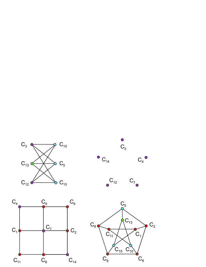
Figure 1: The two basic factorizations of the algebra of the 15 observables/operators of a two-qubit system. A 9+6 factorization (left) corresponds geometrically to the split-up of our sub-configuration of $P_{1}(M_{2}(GF(2)))$ into the projective line over $GF(2)\times GF(2)$ (bottom) and a couple of projective lines over $GF(4)$ having two points in common (top). A 10+5 one (right) corresponds, as also demonstrated in a different way in Fig. 2, to the partition of the generalized quadrangle into one of its ovoids (top) and the Petersen graph (bottom). In both the cases, two points/observables are joined by a line-segment only if they are neighbor/commute and the color is used to illustrate how the two factorizations relate to each other.

The second interpretation involves a generalized quadrangle, a rank two point-line incidence geometry where two points share at most one line and where for any point $X$ and a line ${\cal L}$, $X\notin{\cal L}$, there exists exactly one line through $X$ which intersect ${\cal L}$.^16-20 The generalized quadrangle associated with our observables is of order two, i. e., the one where every line contains three points and every point is on three lines. Such a quadrangle has, indeed, 15 points (and, because of its self-duality, the same number of lines), each of which is joined by a line with other six (Fig. 2, left). If one removes from this quadrangle one of its ovoids, i. e., a set of (five) points that has exactly one point in common with every line (Fig. 2, middle), one is left with the set of ten points that form the famous Petersen graph (Fig. 2, right);^19,20 five points of an ovoid answer to nothing but the five mutually distant points of $P_{1}(GF(4))$ and, so, to the five (i. e., the maximum number of) mutually non-commuting observables of two-qubits. If, dually, one removes from the quadrangle a spread, i. e., a set of (five) pairwise disjoint lines that partition the point set, one gets the dual of the Petersen graph (Fig. 3); five lines of a spread represent nothing but the five maximum subsets of three mutually commuting operators each, whose associated bases are mutually unbiased.^10,21 It is a straightforward exercise to associate the points of the quadrangle with the operators/observables $C_{i}$, Eq. (8), in such a way to recover Table 2, after substituting the “$-$”/“$+$” sign for any two points of the quadrangle which are/are not on a common line.

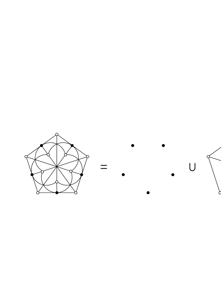
Figure 2: The generalized quadrangle of order two (left) and its factorization into an ovoid (middle) and the “Petersen” part (right). The lines of the quadrangle are illustrated by the straight segments as well as by the segments of circles; note that not every intersection of two segments counts for a point of the quadrangle.

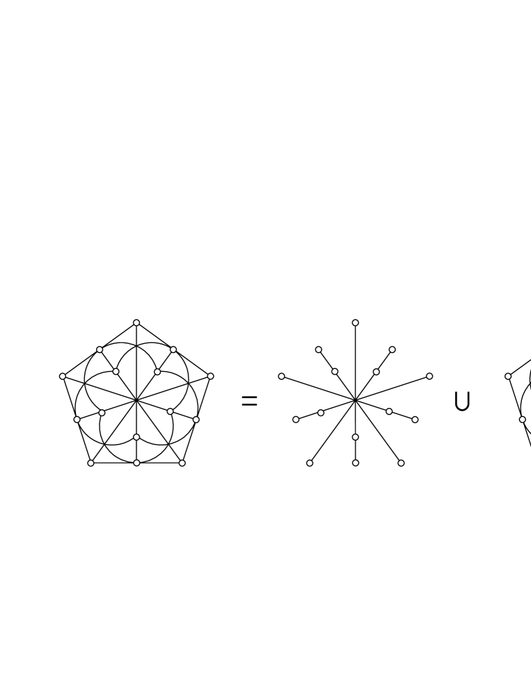
Figure 3: A dual view of the generalized quadrangle of order two (left) as a disjoint union of one of its spreads (middle) and a dual of the Petersen graph, or a 2-spread (right).

To complete this interesting algebraic geometrical picture of two-qubits there remains to be introduced one more important geometrical object. The attentive reader might have noticed that we have already employed two different kinds of the projective lines defined over rings of order four and characteristic two, viz. the line defined over the field $GF(4)$ and that defined over the direct product ring $GF(2)\times GF(2)$; the former was seen to answer to an ovoid of the generalized quadrangle, alias to a set of five mutually non-commuting operators (Fig. 1, right – top), while the latter corresponds to a grid of nine points on six lines, alias to a Mermin’s square of operators (Fig. 1, left – bottom). There, however, exists one more associative ring with unity of order four and characteristic two, namely the (local) factor ring of polynomials $GF(2)[x]/\langle x^{2}\rangle$.^12-14 This ring is also a subring of $M_{2}(GF(2))$, so the corresponding projective line is expected to play a role in our model, too. And this is indeed the case. As demonstrated, for example, in Ref. 6 (Table 3), the projective line $P_{1}(GF(2)[x]/\langle x^{2}\rangle)$ features six points any of which is neighbor to one and distant to the remaining four points, comprising thus three pairs of neighbors. In the set of Pauli operators this configuration is present as the sextuple of operators commuting with a given operator; taking the latter to be, e. g., $C_{13}$, the six operators in question, as readily discerned from Table 2, are $\{$$C_{4}$, $C_{5}$; $C_{7}$, $C_{10}$; $C_{14}$, $C_{15}$$\}$, which indeed form three pairs of commuting members (these pairs being separated from each other by a semicolon). In the generalized quadrangle any such configuration resides as the sextuple of points collinear with a given point. A deeper understanding and a fuller appreciation of this observation is acquired after introducing the concept of a geometric hyperplane. A geometric hyperplane $H$ of a finite geometry is a set of points such that every line of the geometry either contains exactly one point of $H$, or is completely contained in $H$.^20, 22 It is easy to verify that for the generalized quadrangle of order two $H$ is of one of the following three kinds:²² 1) $H_{{\rm ov}}$, an ovoid (there are six such hyperplanes); 2) $H_{{\rm cl}}(X)$, a set of points collinear with a given point $X$, the point itself inclusive (there are 15 such hyperplanes); and 3) $H_{{\rm gr}}$, a grid as defined above (there are 10 such hyperplanes). One thus reveals a perfect parity between the three kinds of the geometric hyperplanes of the generalized quadrangle of order two and the three kinds of the projective lines over the rings of four elements and characteristic two embedded in our sub-configuration of $P_{1}(M_{2}(GF(2)))$, giving rise to the three kinds of the distinguished subsets of the Pauli operators of two-qubits, as summarized in Table 3.

Table 3: Three kinds of the distinguished subsets of the generalized Pauli operators of two-qubits (TQ) viewed as the geometric hyperplanes in the generalized quadrangle of order two (GQ) and/or as the projective lines over the rings of order four and characteristic two living in the projective line $P_{1}(M_{2}(GF(2)))$ (PL).

GQ	$H_{{\rm ov}}$	$H_{{\rm cl}}(X)\setminus\{X\}$	$H_{{\rm gr}}$
PL	$P_{1}(GF(4))$	$P_{1}(GF(2)[x]/\langle x^{2}\rangle)$	$P_{1}(GF(2)\times GF(2))$
TQ	set of five mutually	set of six operators	nine operators of a
	non-commuting operators	commuting with a given one	Mermin’s square

As a final note, it is worth mentioning that the generalized quadrangle of order two also resides in $P_{1}(M_{2}(GF(2)))$ as the projective line over the so-called Jordan system of symmetric two-by-two matrices over $GF(2)$,²³ or, equivalently, as a generic hyperplane section of the Klein quadric in the 5-dimensional projective space over $GF(2)$.²²

We have demonstrated that the basic properties of a system of two interacting spin-1/2 particles are uniquely embodied in the (sub)geometry of a particular projective line, found to be equivalent to the generalized quadrangle of order two. As such systems are the simplest ones exhibiting phenomena like quantum entanglement and quantum non-locality and play, therefore, a crucial role in numerous applications like quantum cryptography, quantum coding, quantum cloning/teleportation and/or quantum computing to mention the most salient ones, our discovery thus not only offers a principally new geometrically-underlined insight into their intrinsic nature, but also gives their applications a wholly new perspective and opens up rather unexpected vistas for an algebraic geometrical modelling of their higher-dimensional counterparts.^24,25

Acknowledgements
The first author thanks Prof. Hans Havlicek (Vienna University of Technology) for bringing to our attention the description of the generalized quadrangle of order two as the projective line over the Jordan system of the ring in question. This work was partially supported by the Science and Technology Assistance Agency under the contract $\#$ APVT–51–012704, the VEGA project $\#$ 2/6070/26 (both from Slovak Republic), the trans-national ECO-NET project $\#$ 12651NJ “Geometries Over Finite Rings and the Properties of Mutually Unbiased Bases” (France) and by the project 1ET400400410 of the Academy of Sciences of the Czech Republic.

References

- [1] Blunck, A., and Havlicek, H., “Projective representations I: Projective lines over a ring,” Abh. Math. Sem. Univ. Hamburg 70, 287–299 (2000).
- [2] Blunck, A., and Havlicek, H., “Radical parallelism on projective lines and non-linear models of affine spaces,” Mathematica Pannonica 14, 113–127 (2003).
- [3] Blunck, A., and Havlicek, H., “On distant-isomorphisms of projective lines,” Aequationes Mathematicae 69, 146–163 (2005).
- [4] Havlicek, H., “Divisible designs, Laguerre geometry, and beyond,” Quaderni del Seminario Matematico di Brescia 11, 1–63 (2006).
- [5] Herzer, A., “Chain geometries,” in Handbook of Incidence Geometry, edited by F. Buekenhout (Elsevier, Amsterdam, 1995), pp. 781–842.
- [6] Saniga, M., Planat, M., Kibler, M. R., and Pracna, P., “A classification of the projective lines over small rings,” Chaos, Solitons Fractals, submitted, math.AG/0606500.
- [7] Saniga, M., and Planat, M., “On the fine structure of the projective line over GF(2) GF(2) GF(2),” Chaos, Solitons Fractals, in press, math.AG/0604307.
- [8] Saniga, M., and Planat, M., “The projective line over the finite quotient ring GF(2)[]/ and quantum entanglement. Theoretical background,” Theoretical and Mathematical Physics, accepted, quant-ph/0603051.
- [9] Saniga, M., Planat, M., and Minarovjech, M., “The projective line over the finite quotient ring GF(2)[]/ and quantum entanglement. The Mermin “magic” square/pentagram,” Theoretical and Mathematical Physics, accepted, quant-ph/0603206.
- [10] Planat, M., Saniga, M., and Kibler, M. R., “Quantum entanglement and finite ring geometry,” SIGMA 2, Paper 066 (2006), quant-ph/0605239.
- [11] Saniga, M., Planat, M., and Pracna, P., “A classification of the projective lines over small rings II. Non-commutative case,” math.AG/0606500.
- [12] Fraleigh, J. B., A First Course in Abstract Algebra (Addison-Wesley, Reading, 1994), pp. 273–362.
- [13] McDonald, B. R., Finite Rings with Identity (Marcel Dekker, New York, 1974).
- [14] Raghavendran, R., “Finite associative rings,” Comp. Mathematica 21, 195–229 (1969).
- [15] Nöbauer, C., The book of the rings — part I, 2000, preprint available online at http://www.algebra.uni-linz.ac.at/noebsi/pub/rings.ps, pp. 433 and 531.
- [16] Van Maldeghem, H., Generalized Polygons (Birkhäuser, Basel, 1998).
- [17] Polster, B., and Van Maldeghem, H., “Some constructions of small generalized polygons,” Journal of Combinatorial Theory A96, 162–179 (2001).
- [18] Polster, B., A Geometrical Picture Book (Springer, New York, 1998).
- [19] Polster, B., “Pretty pictures of geometries,” Bull. Belg. Math. Soc. 5, 417–425 (1998).
- [20] Polster, B., Schroth, A. E., and Van Maldeghem, H., “Generalized flatland,” Math. Intelligencer 23, 33–47 (2001).
- [21] Lawrence, J., Brukner, Č., and Zeilinger, A., “Mutually unbiased binary observable sets on N qubits,” Physical Review A 65, 032320 (2002).
- [22] Payne, S. E., and Thas, J. A., Finite Generalized Quadrangles (Pitman, Boston–London-Melbourne, 1984).
- [23] Havlicek, H., “From pentacyclic coordinates to chain geometries, and back,” Mitt. Math. Ges. Hamburg, in press.
- [24] Saniga, M., and Planat, M., “Multiple qubits as symplectic polar spaces of order two,” quant-ph/0612179.
- [25] Planat, M., and Saniga, M., “On the Pauli graphs relevant to -qudits,” in preparation.