Lissajous curves and semiclassical theory: The two-dimensional harmonic oscillator

Abstract

The semiclassical treatment of the two-dimensional harmonic oscillator provides an instructive example of the relation between classical motion and the quantum mechanical energy spectrum. We extend previous work on the anisotropic oscillator with incommensurate frequencies and the isotropic oscillator to the case with commensurate frequencies for which the Lissajous curves appear as classical periodic orbits. Because of the three different scenarios depending on the ratio of its frequencies, the two-dimensional harmonic oscillator offers a unique way to explicitly analyze the role of symmetries in classical and quantum mechanics.

I Introduction

In 1940 J. M. Jauch and E. L. Hill discussed the relation between symmetries and degeneracies in the spectra of quantum systems. As examples they considered the hydrogen problem, the two-dimensional Kepler problem, and the isotropic harmonic oscillator, but the two-dimensional anisotropic harmonic oscillator resisted their analysis. The authors concluded “We feel, however, that the difficulties encountered in this relatively simple problem throw question on the true interpretation of classical multiply-periodic motions in quantum mechanics.” jauch40

Although the problem is now understood on a group theoretical level, louck73 ; krame75 ; moshi75 the remark by Jauch and Hill motivates us to study the relation between the motion of a classical anisotropic oscillator with commensurate frequencies and its quantum mechanical energy spectrum. This link is provided by semiclassical theory gutzw98 which relates the density of states to properties of the classical periodic orbits. We will restrict the discussion to the two-dimensional case where harmonic potentials already provide three different scenarios for periodic orbits.

For the isotropic harmonic oscillator all orbits are periodic and constitute a continuous family of which two representatives are depicted in Fig. 1(a). Any two distinct periodic orbits can be deformed continuously into each other via other periodic orbits. The situation is different for an anisotropic harmonic oscillator with incommensurate frequencies where only the two normal modes shown in Fig. 1(b) correspond to periodic orbits. The most interesting classical dynamics is exhibited by the harmonic oscillator with commensurate frequencies of which an example is shown in Fig. 1(c). Here, Lissajous curves appear as additional periodic orbits that form a continuous family. These trajectories, which will play an important role in the following, take their name after Jules Antoine Lissajous who gave an extensive discussion of these curves in a study aimed at a comparison of the relative frequencies of two tuning forks. lissa57 Previous work addressing these curves should not be forgotten.crowe81

Figure 1: Examples of the periodic orbits of a two-dimensional harmonic oscillator. The dashed line corresponds to an equipotential line. (a) Isotropic harmonic oscillator. (b) Anisotropic harmonic oscillator with incommensurate frequencies. In this case only the two orbits shown are periodic. (c) Anisotropic harmonic oscillator with commensurate frequency ratio 1:2. In contrast to the case with incommensurate frequencies, Lissajous curves become possible.

It has been proven that semiclassical theory gives the exact expression for the density of states of an isotropiccreag96 as well as for the incommensurate harmonic oscillator.brack95 An interesting property of the harmonic oscillator is that the appropriate limit from incommensurate to commensurate frequencies yields the correct density of states even for the commensurate harmonic oscillator,brack95 although only two periodic orbits are explicitly taken into account. Although taking such a limit considerably simplifies the calculation, it is unsatisfying that a full analysis of the density of states based on all the classical periodic orbits is lacking. Furthermore, a complete account for the symmetries of the commensurate anisotropic harmonic oscillator is not possible without the Lissajous curves. As we will show, the proper treatment of all the periodic orbits of the commensurate anisotropic harmonic oscillator yields the exact density of states and the exact symmetry reduced densities of states. Our analysis thus closes the last lacuna left in the semiclassical treatment of the two-dimensional harmonic oscillator. This system now lends itself well to illustrating the relation between classical dynamics and the symmetry properties of the quantum mechanical energy spectrum.

II The energy spectrum in terms of classical mechanics: the incommensurate harmonic oscillator

Among the three types of two-dimensional harmonic oscillators depicted in Fig. 1, the relation between the quantum mechanical density of states and classical properties is most readily established for the incommensurate harmonic oscillator. The Hamiltonian of a particle of mass $m$ moving in a two-dimensional harmonic potential with eigenfrequencies $\omega_{1}$ and $\omega_{2}$ is given by

$$H=\frac{p_{1}^{2}}{2m}+\frac{m}{2}\omega_{1}^{2}q_{1}^{2}+\frac{p_{2}^{2}}{2m}+\frac{m}{2}\omega_{2}^{2}q_{2}^{2}.$$ (1)

We first use the fact that the total Hamiltonian $H$ can be decomposed into two contributions $H_{1}(q_{1},p_{1})$ and $H_{2}(q_{2},p_{2})$ describing two uncoupled one-dimensional harmonic oscillators. From the classical density of states of the $i$th normal mode,

$$\bar{\rho}_{i}(E)=\!\int\frac{dq_{i}dp_{i}}{2\pi\hbar}\delta\Big{(}E-\frac{p_{i}^{2}}{2m}-\frac{m}{2}\omega_{i}^{2}q_{i}^{2}\Big{)}=\frac{1}{\hbar\omega_{i}},$$ (2)

the classical density of states of the two-dimensional oscillator is obtained by the convolution

$$\bar{\rho}(E)=\!\int_{0}^{E}dE^{\prime}\bar{\rho}_{1}(E-E^{\prime})\bar{\rho}_{2}(E^{\prime})=\frac{E}{\hbar^{2}\omega_{1}\omega_{2}}.$$ (3)

The quantum mechanical energy spectrum is given by

$$E_{\nu_{1},\nu_{2}}=\hbar\omega_{1}\Big{(}\nu_{1}+\frac{1}{2}\Big{)}+\hbar\omega_{2}\Big{(}\nu_{2}+\frac{1}{2}\Big{)},$$ (4)

where $\nu_{1},\nu_{2}=0,1,2,\dots$ The corresponding quantum mechanical density of states is

$$\rho(E)=\sum_{\nu_{1},\nu_{2}=0}^{\infty}\delta(E-E_{\nu_{1},\nu_{2}}).$$ (5)

Equation (5) can be interpreted in terms of the classical properties of the incommensurate harmonic oscillator if it is appropriately re-expressed. We perform a Laplace transform of Eq. (5) and find the partition function of the incommensurate harmonic oscillator

$$\mathcal{Z}_{\beta} =\!\int_{0}^{\infty}\!dE\,\rho(E)\exp(-\beta E)$$ (6)

$$=\frac{1}{4\sinh\Big{(}\displaystyle\frac{\hbar\beta\omega_{1}}{2}\Big{)}\sinh\Big{(}\displaystyle\frac{\hbar\beta\omega_{2}}{2}\Big{)}}.$$

The inversion of the Laplace transform by means of a contour integration yields three kinds of contributions from the various poles on the imaginary axis. The double pole at $\beta=0$ gives rise to the classical density of states (3), and the poles at $\beta=\pm i2\pi n/\hbar\omega_{1}$ and $\beta=\pm i2\pi n/\hbar\omega_{2}$ with $n=1,2,\dots$ lead to contributions responsible for the difference between the classical and quantum density of states. The latter can thus be expressed as

$$\rho(E)=\bar{\rho}(E)+\delta\rho_{1}(E)+\delta\rho_{2}(E).$$ (7)

After evaluating the residues, we obtain

$$\delta\rho_{1}(E)=\frac{1}{\pi\hbar}\sum_{r=1}^{\infty}T_{1}\frac{\cos\Big{(}\displaystyle r\frac{2\pi E}{\hbar\omega_{1}}-\frac{\pi}{2}\sigma_{r,1}\Big{)}}{2|\sin(\pi r\omega_{2}/\omega_{1})|},$$ (8)

with

$$\sigma_{r,1}=2r+1+2\Big{[}r\frac{\omega_{2}}{\omega_{1}}\Big{]}.$$ (9)

The quantities $\delta\rho_{2}(E)$ and $\sigma_{r,2}$ are expressed in the same way with the indices $1$ and $2$ interchanged. We have written the expressions in a form that anticipates the following discussion. In particular, we have introduced the periods $T_{i}=2\pi/\omega_{i}$ of the two normal modes and phases $\sigma_{r,i}$. In Eq. (9) $[x]$ denotes the integer part of $x$.

We expect that it should be possible to relate the terms in $\delta\rho_{i}$ to the properties of the two periodic orbits shown in Fig. 1(b). As a motivation we remark that within the Feynman path integral approachfeynm48 all paths joining two points in a given time contribute to the corresponding quantum propagator a phase factor $\exp(iS/\hbar)$, where $S$ is Hamilton’s principal function of the path. For $S\gg\hbar$, we can apply the semiclassical approximationgutzw98 ; remark and find that the path integral is dominated by the stationary points of $S$, that is, the classical paths. Within this approximation even the contribution of quantum fluctuations can be expressed in terms of properties of the classical motion.brack97 ; ingol02

The propagator can be related to the density of states by means of the Green function $G(E)=(E-H)^{-1}$, the Fourier transform of the propagator. From the relation

$$\rho(E) =-\frac{1}{\pi}\lim_{\epsilon\to 0^{+}}\text{Im}\,(\text{Tr}\,[G(E+i\epsilon)])$$ (10)

$$=-\frac{1}{\pi}\lim_{\epsilon\to 0^{+}}\text{Im}\sum_{\nu_{1},\nu_{2}}\frac{1}{E+i\epsilon-E_{\nu_{1},\nu_{2}}},$$

we see that $\rho(E)$ involves the trace over the Green function, so that the initial and final points of the contributing classical paths coincide. Equation (10) contains contributions from very short orbits which yield $\bar{\rho}(E)$ and periodic orbits of finite length contribute to $\delta\rho(E)=\delta\rho_{1}(E)+\delta\rho_{2}(E)$. The latter relation is given by the Gutzwiller trace formula gutzw90 ; brack97 of which Eq. (8) is an example.

These considerations indicate that within the semiclassical approximation the density of states can be expressed in terms of classical properties, but such an expression cannot be expected in general. However, it was shown by Brack and Jainbrack95 that the incommensurate harmonic oscillator is one of the rare cases where the Gutzwiller formula yields the exact density of states. As a consequence, it should be possible to interpret the various terms in Eq. (8) by means of a classical periodic orbit. We will check now that this is the case.

We have already mentioned that the prefactor $T_{1}$ in Eq. (8) represents the period of the first normal mode. The argument of the cosine function in the numerator contains the classical action

$$W_{1}(E)=\!\oint dq_{1}p_{1}=\frac{2\pi E}{\omega_{1}}$$ (11)

of the fundamental periodic orbit along the $q_{1}$ axis for a given energy $H_{1}=E$; we sum over all repetitions counted by $r$.

The denominator is determined by the lateral stability of the periodic orbit as the following argument shows. The equations of motion of a harmonic oscillator can easily be solved, and we find

$$\begin{pmatrix}q_{i}(t)\\ p_{i}(t)\\ \end{pmatrix}=\mathsf{X}_{i}(t)\begin{pmatrix}q_{i}(0)\\ p_{i}(0)\end{pmatrix}$$ (12)

with the matrizant

$$\mathsf{X}_{i}(t)=\begin{pmatrix}\cos(\omega_{i}t)&\displaystyle\frac{\sin(\omega_{i}t)}{m\omega_{i}}\\ -m\omega_{i}\sin(\omega_{i}t)&\cos(\omega_{i}t)\\ \end{pmatrix}.$$ (13)

We again consider the periodic orbit along the $q_{1}$ axis which is specified by the initial conditions $q_{2}(0)=0$ and $p_{2}(0)=0$. We are interested in the evolution of a small lateral perturbation during $r$ oscillations. After the time $rT_{1}$, we find a deviation

$$\begin{pmatrix}\delta q_{2}\\ \delta p_{2}\end{pmatrix}=[\mathsf{X}_{2}(rT_{1})-\openone]\begin{pmatrix}q_{2}(0)\\ p_{2}(0)\end{pmatrix}$$ (14)

in the direction orthogonal to the periodic orbit with respect to the perturbed initial condition. The matrix $\mathsf{X}_{2}(rT_{1})$ thus measures the stability during $r$ repetitions of the first normal mode against a small initial perturbation. It enters the denominator of Eq. (8) by means of its property

$$\sqrt{|\det[\mathsf{X}_{2}(rT_{1})-\openone]|}=2|\sin(\pi r\omega_{2}/\omega_{1})|.$$ (15)

The last quantity requiring interpretation is the Maslov index $\sigma_{r,1}$ defined by Eq. (9). It collects all phases appearing in the evaluation of the stationary phase integral of the first periodic orbit. Because the derivation of Eq. (9) within a semiclassical approach is more demanding, we refer the reader interested in the details to the literature.brack95

We started from an exact expression for the density of states of the incommensurate harmonic oscillator and arrived at a semiclassical interpretation. In contrast, in the following two sections, we will go the opposite way and first derive a semiclassical expression for the density of states of the isotropic harmonic oscillator and the commensurate anisotropic harmonic oscillator by exploiting the system’s classical properties. At the end of each section, we will then compare with the exact quantum mechanical result.

III Semiclassical theory in the presence of a continuous symmetry: the isotropic harmonic oscillator

As we have seen, the semiclassical density of states is intimately related to the classical periodic orbits. Because the incommensurate harmonic oscillator exhibits only two such orbits, its semiclassical density of states is relatively simple to determine.

As the next step toward a semiclassical understanding of the commensurate anisotropic harmonic oscillator, we consider the more complex case of equal frequencies, $\omega_{1}=\omega_{2}=\omega$. The fundamental periods of oscillations along the $q_{1}$- and $q_{2}$-axes are equal, $T_{1}=T_{2}=T=2\pi/\omega$ and from Eq. (13) we find $\mathsf{X}_{2}(rT_{1})=\mathsf{X}_{1}(rT_{2})=\openone$ for any integer $r$, which is related to the fact that any starting point on an energy surface $H=E$ in the four-dimensional phase space leads to a periodic orbit. In particular, the oscillations along the $q_{1}$- and $q_{2}$-axes are still periodic and should contribute to the semiclassical density of states as was the case in Sec. II. However, the denominators in Eq. (8) reflecting the stability of the orbits vanish. The resulting divergences indicate that the evaluation of the propagator within the stationary phase approximation fails because the stationary points are no longer isolated but form a continuous family. A small perturbation of the initial conditions thus leads to another periodic orbit close to the original one. It is even possible to continuously deform the two Lissajous curves depicted in Fig. 1(a) into each other. The existence of a family of periodic orbits is a consequence of the presence of a continuous symmetry that maps a given orbit to a neighboring one. Hence, the relation between the classical properties and the density of states discussed in the Sec. II has to be modified.

To understand the necessary changes, we consider the phase space symmetries of the isotropic harmonic oscillator and define the quantities golds80 ; mcint59

$$J_{1} =\frac{1}{2\omega}\Big{(}\frac{p_{1}p_{2}}{m}+m\omega^{2}q_{1}q_{2}\Big{)}$$ (16a)

$$J_{2} =\frac{1}{2}(q_{1}p_{2}-q_{2}p_{1})$$ (16b)

$$J_{3} =\frac{1}{2\omega}\Big{(}\frac{p_{1}^{2}}{2m}+\frac{m}{2}\omega^{2}q_{1}^{2}-\frac{p_{2}^{2}}{2m}-\frac{m}{2}\omega^{2}q_{2}^{2}\Big{)},$$ (16c)

for which we find the Poisson brackets

$$\{J_{i},J_{j}\}=\epsilon_{ijk}J_{k},$$ (17)

where $\epsilon_{ijk}$ is the completely antisymmetric tensor. Two of the $J_{i}$ have an obvious physical meaning. $J_{2}$ is proportional to the angular momentum and generates rotations around the axis perpendicular to the $q_{1}$-$q_{2}$ plane. It thus accounts for the rotational symmetry of the isotropic oscillator in real space. $J_{3}$ represents the difference of the energies of the normal modes. $J_{2}$ and $J_{3}$ are conserved quantities as can be verified explicitly by evaluating the Poisson bracket with the Hamiltonian of the isotropic harmonic oscillator. Because $J_{1}$ results from the Poisson bracket of two conserved quantities, it is a constant of the motion as well. We also have

$$J_{1}^{2}+J_{2}^{2}+J_{3}^{2}=\Big{(}\frac{E}{2\omega}\Big{)}^{2}.$$ (18)

From the quantum version of Eq. (17)

$$[J_{i},J_{j}]=i\hbar\epsilon_{ijk}J_{k}$$ (19)

the relation to spin 1/2 is evident. Both the spin 1/2 and the isotropic two-dimensional harmonic oscillator exhibit a SU(2) symmetry, which indicates how the periodic orbits of the isotropic harmonic oscillator can be classified.

It is useful to recall the concept of a Bloch sphere. If we introduce spherical coordinates, every state of a spin 1/2 can be expressed in terms of the orthogonal basis states $|{\uparrow}\rangle$ and $|{\downarrow}\rangle$ as

$$|\psi\rangle=\cos(\theta/2)|{\uparrow}\rangle+\sin(\theta/2)e^{i\varphi}|{\downarrow}\rangle,$$ (20)

where $\theta$ runs from $0$ to $\pi$ and $\varphi$ from $0$ to $2\pi$. This representation provides a one-to-one mapping between the spin states and the points on a sphere. In particular, the cartesian coordinates $x_{i}$ of a point on the Bloch sphere are proportional to the spin expectation values $\langle S_{i}\rangle$. We also note that the spin operators serve as generators of rotations on the Bloch sphere so that an arbitrary state can be generated by starting from a given initial state, for example, $|{\uparrow}\rangle$.

In close analogy, there is a one-to-one correspondence between a point $\hat{r}$ on a unit sphere and a classical periodic orbit of the isotropic harmonic oscillator. The orbit is uniquely characterized by the values of the conserved quantities in Eq. (16) which can be expressed by $\vec{J}=(E/2\omega)\hat{r}$. According to Eq. (16c), the latitude on the Bloch sphere determines the distribution of the energy between the two oscillation modes along the coordinate axes. The north and south pole of the Bloch sphere correspond to extremal values of $J_{3}$, that is, to an oscillation along one of the coordinate axes. The equator represents all periodic orbits where the energy is equally shared between the two modes. The position on the equator determines the relative phase of the two oscillatory motions.

In four-dimensional phase space these three conserved quantities leave one degree of freedom undetermined, which corresponds to the motion along the periodic orbit generated by the Hamiltonian. In analogy to spin 1/2, all periodic orbits can be generated from a given periodic orbit by means of the conserved quantities in Eq. (16).

A generalized trace formula that takes into account continuous symmetries was given in Refs. creag91, ; creag92, ; murat03, . If we adapt Eq. (5.1) in Ref. creag92, to the special case of an isotropic harmonic oscillator where all periodic orbits are members of a single two-parametric family, we find that the deviation from the classical density of states of the semiclassical (sc) density of states is

$$\delta\rho_{\rm sc}(E)=\frac{TV|\vec{J}|}{2(\pi\hbar)^{2}}\sum_{r=1}^{\infty}\cos\Big{(}r\frac{W}{\hbar}-(\sigma_{r}+1)\frac{\pi}{2}\Big{)}.$$ (21)

As before, Eq. (21) is valid only for positive energies. It resembles Eq. (8) in several respects, but there are differences due to the existence of a family of periodic orbits. We first remark that all members of the family share the same action $W$, period $T$, and Maslov indices $\sigma_{r}$ for $r$ repetitions of the periodic orbit. Therefore, apart from the factor $T=2\pi/\omega$, which arises from the integral along a periodic orbit, an additional factor $V|\vec{J}|$ appears as a result of the integration over the family. The volume occupied by the family is given by the surface of the Bloch sphere $V=4\pi$. The factor $|\vec{J}|=E/2\omega$ reflects our choice for the basis of the Lie algebra characterizing the symmetry group. creag92 ; creag96 A comparison of Eqs. (8) and (21) reveals that the factor derived from stability considerations in Eq. (15) is missing for the isotropic harmonic oscillator. This difference should be expected because every perturbation of a periodic orbit will lead to another periodic orbit so that in contrast to the incommensurate harmonic oscillator, the question of lateral stability for the isotropic harmonic oscillator does not make sense.

We note that the change in the symmetry properties prevents us from deriving the Maslov index from the expression Eq. (9) by simply setting $\omega_{1}=\omega_{2}$. The result for the incommensurate harmonic oscillator has to be modified by an additional symmetry-induced contributioncreag96 ; doll04 $\Delta\sigma=-2$ so that the Maslov index of the isotropic harmonic oscillator becomes

$$\sigma_{r}=4r-1.$$ (22)

Substituting the expressions for the period $T$, the surface of the Bloch sphere $V$, and the factor $|\vec{J}|$ given below Eq. (21) as well as the action $W=2\pi E/\omega$ and the Maslov index (22) in the generalized trace formula (21), we arrive at the semiclassical correction to the classical density of states for the isotropic harmonic oscillator

$$\delta\rho_{\rm sc}(E) =\frac{2E}{\hbar^{2}\omega^{2}}\sum_{r=1}^{\infty}\cos\Big{(}r\frac{2\pi E}{\hbar\omega}\Big{)}$$ (23)

$$=\frac{E}{\hbar^{2}\omega^{2}}\Big{[}\sum_{n=-\infty}^{\infty}\delta\Big{(}\frac{E}{\hbar\omega}-n\Big{)}-1\Big{]},$$

In the second step, we have used the Poisson resummation formula. After adding the classical density of states (3) we recover for positive energies the exact quantum mechanical result as was the case for the incommensurate harmonic oscillator.

IV Semiclassical theory for the commensurate anisotropic harmonic oscillator

IV.1 From the anisotropic to the isotropic oscillator

We now turn to the case of different but commensurate frequencies where isolated periodic orbits coexist with a family of periodic orbits. A key point for understanding the properties of a commensurate anisotropic harmonic oscillator, both with respect to group theory and to its semiclassical treatment, is the mapping to the isotropic harmonic oscillator. With the spatial symmetries in mind, it might come as a surprise that such a mapping should be possible because an anisotropic harmonic oscillator does not obey the rotational symmetry characteristic for the isotropic case. In fact, real space symmetries are not useful here and we will be required to consider symmetries in phase space.

To motivate the relation between the commensurate anisotropic harmonic oscillator and the isotropic harmonic oscillator, we consider the energy spectrum of a harmonic oscillator with commensurate frequencies satisfying $k_{1}\omega_{1}=k_{2}\omega_{2}=\omega$, where $k_{1}$ and $k_{2}$ are assumed to be integers without a common divisor. It is instructive to express the quantum numbers $\nu_{i}$ appearing in the energy spectrum (4) in the commensurate case as $\nu_{i}=n_{i}k_{i}+\lambda_{i}$, where $\lambda_{i}=0,1,\dots,k_{i}-1$ and $n_{i}=0,1,2,\dots$,louck73 so that the energy spectrum takes the form

$$E=\hbar\omega\Big{(}n_{1}+n_{2}+\frac{\lambda_{1}}{k_{1}}+\frac{\lambda_{2}}{k_{2}}+\frac{k_{1}+k_{2}}{2k_{1}k_{2}}\Big{)}.$$ (24)

These eigenenergies can be viewed as describing $k_{1}k_{2}$ sets of spectra of a two-dimensional isotropic harmonic oscillator shifted in energy relative to each other so that the isotropic harmonic oscillator appears to be represented multiple times in the commensurate anisotropic harmonic oscillator. This interpretation motivates us to seek a mapping between these two systems and also to find their classical counterparts.

Because we are interested in the phase space structure, we briefly recall the results of the Hamilton-Jacobi method applied to the harmonic oscillator.golds80 The action $W_{i}$ is given by Eq. (11) and the corresponding angle can be expressed as

$$\vartheta_{i}=\arctan\Big{(}\frac{m\omega q_{i}}{k_{i}p_{i}}\Big{)}.$$ (25)

The motion of the harmonic oscillator thus takes place on a torus that is parametrized by the angles $\vartheta_{1}$ and $\vartheta_{2}$. The size of the torus is determined by the actions $W_{1}$ and $W_{2}$. The solid line in Fig. 2(a) depicts the motion on the torus for a commensurate anisotropic harmonic oscillator with $k_{1}=5$ and $k_{2}=4$.

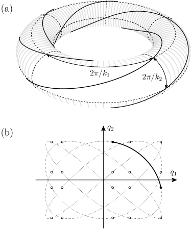
Figure 2: The motion of a commensurate anisotropic harmonic oscillator with $k_{1}=5$ and $k_{2}=4$ is depicted in action-angle variables and in spatial coordinates. (a) The full line represents a trajectory of the commensurate anisotropic harmonic oscillator on a torus in phase space parametrized by action-angle variables. The white section indicates one of the $k_{1}k_{2}$ elementary cells delineated by the dashed lines. Each cell after identification of its opposite borders corresponds to an isotropic harmonic oscillator. (b) The projection of the trajectory onto real space leads to a Lissajous curve. The small circles indicate the positions where the trajectory crosses from one elementary cell into another one. The full line represents the trajectory in one such cell.

According to Eq. (11), the mapping from a commensurate anisotropic harmonic oscillator to an isotropic harmonic oscillator can be achieved by the transformationlouck73 ; moshi75 ; krame75

$$W_{i} \mapsto\widetilde{W}_{i}=\frac{W_{i}}{k_{i}}$$ (26a)

$$\vartheta_{i} \mapsto\widetilde{\vartheta}_{i}=k_{i}\vartheta_{i}.$$ (26b)

The definition of the new angles $\widetilde{\vartheta}_{i}$ ensures that the transformation is canonical. Remarkably, the different angles $\vartheta_{i}+\lambda_{i}2\pi/k_{i}$, $\lambda_{i}=0,1,\ldots k_{i}-1$ are mapped onto the same angle $\widetilde{\vartheta}_{i}$, because we have to identify $\widetilde{\vartheta}_{i}+2\pi$ with $\widetilde{\vartheta}_{i}$ as usual. The transformation (26) thus leads to a folding of phase space into $k_{i}$ sheets for each mode $i$. This folding is necessary to turn the commensurate anisotropic harmonic oscillator into an isotropic harmonic oscillator, because it ensures that the original periods $T_{i}=2\pi k_{i}$ of the normal modes are mapped onto equal periods $\widetilde{T}=2\pi$. After the canonical transformation (26) we now have $k_{1}k_{2}$ isotropic harmonic oscillators instead of one commensurate anisotropic harmonic oscillator. Figure 2(a) illustrates the transformation (26). The white cell covering the interval $2\pi/k_{i}$ for angle $\vartheta_{i}$ turns into a square of side length $2\pi$ by the transformation (26). By identifying opposite sides of the cell, a new torus is formed on which the motion of an isotropic harmonic oscillator in phase space takes place. Because the original torus contains $k_{1}k_{2}$ such cells marked by the dashed lines, Eq. (26) provides a mapping from a commensurate anisotropic harmonic oscillator to $k_{1}k_{2}$ isotropic harmonic oscillators.

IV.2 Symmetries of the commensurate anisotropic harmonic oscillator

We can now analyze the symmetries present in the commensurate anisotropic harmonic oscillator: There exists a discrete symmetry associated with the mapping from the commensurate anisotropic harmonic oscillator to multiple copies of isotropic harmonic oscillators. In addition, according to Sec. III, each isotropic harmonic oscillator possesses the continuous symmetry SU(2). The presence of the discrete symmetry is a direct consequence of the folding of phase space discussed in Sec. IV.1. We can introduce complex variables $z_{i}=\sqrt{W_{i}}\exp(-i\vartheta_{i})$ to write the transformation (26) as

$$\tilde{z}_{i}=\frac{|z_{i}|}{\sqrt{k_{i}}}\Big{(}\frac{z_{i}}{|z_{i}|}\Big{)}^{k_{i}},$$ (27)

which is invariant under $z_{i}\mapsto z_{i}\exp(2\pi i/k_{i})$. Hence, the symmetry operations consist of rotations in the complex plane by multiples of $2\pi/k_{i}$. The rotations form a symmetry group $\mathcal{C}_{i}=\{c_{{\rm g},i},c^{2}_{{\rm g},i},\ldots,c^{k_{i}}_{{\rm g},i}\}$ generated by the fundamental rotation $c_{{\rm g},i}$ by $2\pi/k_{i}$. The identity is given by the group element $c^{k_{i}}_{{\rm g},i}$ which leads to a rotation by $2\pi$. Taking together the rotations for both oscillator modes, we arrive at the product group $\mathcal{C}=\mathcal{C}_{1}\times\mathcal{C}_{2}$ containing $k_{1}k_{2}$ elements and generated by the element $c_{\rm g}=c_{{\rm g},1}\times c_{{\rm g},2}$. For later use we note that the irreducible representationsremark2 ; tinkh64 of $\mathcal{C}$ can be labeled by a tupel $(\lambda_{1},\lambda_{2})$ with $\lambda_{i}=0,1,\ldots,k_{i}-1$. The characterremark2 $\mathcal{X}$ of the group element $c_{\rm g}$ in the representation $(\lambda_{1},\lambda_{2})$ is given by $\mathcal{X}_{\lambda_{1},\lambda_{2}}(c_{\rm g})=\exp(2\pi i\zeta_{\lambda_{1},\lambda_{2}})$, where we have introduced the phases

$$\zeta_{\lambda_{1},\lambda_{2}}=\frac{\lambda_{1}}{k_{1}}+\frac{\lambda_{2}}{k_{2}}.$$ (28)

We emphasize that here we are concerned with a phase space symmetry. In real space, a symmetry operation would map a segment of a Lissajous curve such as the solid curve in Fig. 2(b) onto one of the other segments (delimited in the figure by two small circles) of the same Lissajous curve. By starting from a fundamental segment, we can arrive at the complete Lissajous curve by successively applying the generator $c_{\rm g}$ of the group $k_{1}k_{2}$ times. In the Bloch sphere picture, each segment is represented as a point on a Bloch sphere corresponding to one isotropic harmonic oscillator. Because the commensurate anisotropic harmonic oscillator has been mapped onto $k_{1}k_{2}$ isotropic harmonic oscillators, a complete Lissajous curve corresponds to one point on each of $k_{1}k_{2}$ Bloch spheres. The mapping between two segments of a Lissajous curve then implies a jump from one Bloch sphere to another one.

IV.3 Construction of the semiclassical density of states

For the semiclassical treatment of the commensurate anisotropic harmonic oscillator, we need to know which periodic orbits come in families and which ones are isolated. We start with a general Lissajous curve where both one-dimensional harmonic oscillators along the $q_{1}$- and $q_{2}$-axes have to return to the starting point of their oscillations at the same time. Because their fundamental periods are equal to $T_{i}=2\pi k_{i}/\omega$ and $k_{1}$ and $k_{2}$ are assumed to have no common divisor, the fundamental period for a Lissajous curve is given by $T=2\pi k_{1}k_{2}/\omega$. A Lissajous curve in configuration space corresponds to a periodic orbit in full phase space where $\mathsf{X}_{1}(2\pi k_{1}k_{2})=\mathsf{X}_{2}(2\pi k_{1}k_{2})=\openone$. By varying the energy difference between the two oscillators and the relative phase of their oscillations, all possible Lissajous curves are obtained, including their degeneracies into oscillations along the coordinate axes.

During the time $T$, $k_{2}$ oscillations along the $q_{1}$ axis and $k_{1}$ oscillations along the $q_{2}$ axis occur. Hence, all oscillations along the $q_{1}$ ($q_{2}$) axis with fundamental period $T_{1}$ ($T_{2}$) that are not repeated $k_{2}$ ($k_{1}$) times or multiples thereof are not members of the family of Lissajous curves. They cannot be deformed continuously into a Lissajous curve nor into each other and lie isolated in phase space. Accordingly, for the isolated periodic orbits, one of the matrizants $\textsf{X}_{1}$ or $\textsf{X}_{2}$ becomes equal to unity but not both.

These different types of periodic orbits lead to a decomposition of the semiclassical density of states of the commensurate anisotropic harmonic oscillator into four terms

$$\rho_{\rm sc}(E)=\bar{\rho}(E)+\delta\rho_{\Gamma}(E)+\delta\rho_{1}(E)+\delta\rho_{2}(E),\quad(E>0)$$ (29)

where $\bar{\rho}$ is the classical density of states (3). $\delta\rho_{\Gamma}$ accounts for the contribution of the family of Lissajous curves denoted by $\Gamma$ here and in the following, and the last two terms arise from the contribution of the isolated periodic orbits. The latter can be treated in the same way as the two periodic orbits of the incommensurate harmonic oscillator in Sec. II. From Eq. (8) we find after substituting the corresponding period and the Maslov index (9):

$$\delta\rho_{1}(E)=\frac{k_{1}}{\hbar\omega}\sum_{r=1}^{\infty}{}^{\prime}(-1)^{r}\frac{\sin\Big{(}\displaystyle k_{1}r\frac{2\pi E}{\hbar\omega}\Big{)}}{\sin(\pi rk_{1}/k_{2})}.$$ (30)

The prime indicates that the sum is restricted to the isolated periodic orbits, that is, those repetitions $r$ for which the denominator does not vanish; $\delta\rho_{2}(E)$ is obtained by interchanging $k_{1}$ and $k_{2}$ in Eq. (30).

To determine the contribution $\delta\rho_{\Gamma}$ of the family of Lissajous curves to the density of states, we make use of the discrete symmetry presented in Sec. IV.2. The mapping to the isotropic harmonic oscillator will allow us to take advantage of the results of Sec. III.

The presence of a symmetry imposes a structure on the dynamical equations that lets us consider the kinematics in a reduced space. In a quantum mechanical picture, the full Hilbert space of the problem can be decomposed into invariant subspaces corresponding to the irreducible representations of the underlying symmetry group.tinkh64 As a consequence, the solution of the Schrödinger equation that is restricted to these subspaces yields symmetry-reduced spectra.

A semiclassical treatment of this idea was used in Refs. lauri91, –robbi89, for discrete symmetries in configuration space and in Ref. creag93, for continuous symmetries. Although the commensurate anisotropic harmonic oscillator exhibits a discrete as well as a continuous symmetry, we use symmetry reduction only for the discrete group $\mathcal{C}$. After we have determined the symmetry reduced densities of states, we will sum over all irreducible representations. It can be generally shown that the full spectrum is constructed in this way.robbi89 ; creag93 ; doll04

An orthogonal projection corresponding to the irreducible representation $(\lambda_{1},\lambda_{2})$ can be achieved using the projection operator tinkh64

$$P_{(\lambda_{1},\lambda_{2})}=\frac{d_{\lambda_{1},\lambda_{2}}}{|\mathcal{C}|}\sum_{c}\mathcal{X}^{\ast}_{\lambda_{1},\lambda_{2}}\!(c)\>U(c),$$ (31)

where $U(c)$ is the unitary operator describing the action of the group element $c$ in Hilbert space. $d_{\lambda_{1},\lambda_{2}}$ is given by the dimension of the irreducible representation which in our case is always equal to one.remark2 By this projection the Green function $G(E)$, its trace and, in view of Eq. (10), the density of states are modified accordingly.doll04 The reduced densities of states corresponding to the irreducible representation $(\lambda_{1},\lambda_{2})$ are found to be

$$\delta\rho_{\Gamma}^{(\lambda_{1},\lambda_{2})}(E)$$ (32)

$$=\frac{2E}{\hbar^{2}\omega^{2}}\sum_{r=1}^{\infty}\cos\Big{[}2\pi r\Big{(}\frac{E}{\hbar\omega}-\zeta_{\lambda_{1},\lambda_{2}}\Big{)}-(\tilde{\sigma}_{r}+1)\frac{\pi}{2}\Big{]}.$$

The phases $\zeta_{\lambda_{1},\lambda_{2}}$ are defined in Eq. (28) and arise from the character $\mathcal{X}$ present in Eq. (31). As we will see in the discussion of Fig. 3, this phase is responsible for a relative shift of the reduced energy spectra.

Figure 3: Density of states of the commensurate anisotropic harmonic oscillator with frequency ratio 3:2. (a) Contribution of the classical density of states and the family of periodic orbits. The six different symmetry classes $(\lambda_{1},\lambda_{2})$ that repeat themselves periodically are indicated. (b) The contribution arising from the isolated periodic orbits. (c) The total density of states of the commensurate anisotropic harmonic oscillator.

The expression (32) can also be interpreted within a classical picture, where the available phase space is reduced to a primitive cell, for example, the white area depicted in Fig. 2(a). The motion in full phase space may be recovered using symmetry operations. Correspondingly, a Lissajous curve of the commensurate anisotropic harmonic oscillator is reduced to a fundamental segment, for example, the full line in Fig. 2(b). The endpoints of such a segment are identified, thus yielding a periodic orbit of the isotropic harmonic oscillator whose continuous SU(2) symmetry still remains. We therefore can directly apply the results of Sec. III. It turns out that the contribution to the semiclassical density of states of the $r$th repetition of such an orbit acquires an additional phase given by the character of the group element $c_{\rm g}^{r}$. This group operation is needed to close the corresponding partial orbit in full phase space and, within a classical picture, can be viewed as the origin of the shift of the reduced energy spectra mentioned previously.

It remains to determine the Maslov index $\tilde{\sigma}_{r}$ of an orbit segment in Eq. (32). Let us consider as a representative of the whole family the oscillation along the $q_{1}$ axis. We recall that only $k_{2}$ repetitions of the fundamental periodic orbit form a member of the family. We also have to keep in mind that we are now working in reduced dynamics where the $k_{1}k_{2}$th part of a periodic orbit of a commensurate anisotropic harmonic oscillator appears as a periodic orbit of an isotropic harmonic oscillator. We therefore have to replace $r$ in Eq. (9) by $rk_{2}/k_{1}k_{2}$. If we add the correction $\Delta\sigma=-2$ as in the derivation of Eq. (22) for the isotropic harmonic oscillator, we obtain

$$\tilde{\sigma}_{r}=2r\frac{k_{1}+k_{2}}{k_{1}k_{2}}-1.$$ (33)

With Eqs. (3), (30), (32), and (33) we have all the information needed to construct the full density of states (29). We proceed in two steps as illustrated in Fig. 3 for the special case of $k_{1}=3$ and $k_{2}=2$. First, we note that the symmetry reduction performed for the family of periodic orbits can also be applied to the classical density of states $\bar{\rho}(E)$. As we have seen, the reduced dynamics takes place in only the $k_{1}k_{2}$th part of the original phase space volume. Correspondingly, the classical density of states contributes to each reduced density of states only $\bar{\rho}(E)/k_{1}k_{2}$. We add this contribution to each of the reduced densities of states arising from the family of periodic orbits and arrive at $k_{1}k_{2}$ series of delta peaks with a height increasing linearly with energy. The density of states resulting from these two contributions is shown in Fig. 3(a) where $k_{1}k_{2}=6$ irreducible representations lead to a corresponding number of series of delta peaks shifted relative to each other in energy.

This density of states has to be corrected by the contribution $\delta\rho_{1}(E)+\delta\rho_{2}(E)$ arising from the isolated orbits (see Fig. 3(b)). The sum of all contributions is shown in Fig. 3(c), where we can check that the eigenenergies with their degeneracies are correctly generated. We remark that the first two peaks of Fig. 3(a) are canceled by the first two peaks in Fig. 3(b), so that the ground state energy $5\hbar\omega/12$ is associated with the irreducible representation (0,0).

Although this example indicates that the semiclassical treatment reproduces the spectrum of the commensurate anisotropic harmonic oscillator, it is useful to explicitly perform the sum over the reduced densities of states (32)

$$\delta\rho_{\Gamma}(E)=\sum_{\lambda_{1}=0}^{k_{1}-1}\sum_{\lambda_{2}=0}^{k_{2}-1}\delta\rho_{\Gamma}^{(\lambda_{1},\lambda_{2})}(E).$$ (34)

By interchanging the double sum with the sum over all repetitions $r$ in Eq. (32), it is seen that Eq. (34) vanishes except when $r$ is a multiple of $k_{1}k_{2}$. Therefore only such orbits of the reduced dynamics actually contribute, which are repeated $k_{1}k_{2}$ times. As expected, these orbits are exactly the full Lissajous curves.

We may now replace the summation index $r$ in Eq. (32) by $r=k_{1}k_{2}k$ where $k=1,2,\ldots$, and arrive at

$$\delta\rho_{\Gamma}(E)$$ (35)

$$=\frac{2Ek_{1}k_{2}}{\hbar^{2}\omega^{2}}\sum_{k=1}^{\infty}(-1)^{k(k_{1}+k_{2})}\cos\Big{(}kk_{1}k_{2}\frac{2\pi E}{\hbar\omega}\Big{)}.$$

Adding the classical density of states and the contributions of the isolated orbits, Eq. (29) yields the exact density of states of the commensurate anisotropic harmonic oscillator.brack95 This result can be checked by summing the exact partition function and taking the inverse Laplace transform as we did for the incommensurate harmonic oscillator in Sec. II.

V Conclusions

The harmonic oscillator is a unique system with fundamental applications in many areas in physics. It admits exact solutions that are often helpful in the illustration of theoretical approaches and methods. As we have seen, it is particularly interesting to consider a semiclassical treatment where a relation between classical and quantum properties can be established. Beyond the interesting different scenarios for periodic orbits provided by the two-dimensional harmonic oscillator, this system beautifully illustrates the relation between classical phase space symmetries and quantum degeneracies.

VI Suggested problems

Problem 1. The conserved quantities $J_{k}$ of the isotropic harmonic oscillator defined in Eq. (16) can be interpreted as generators of infinitesimal transformations. For example, $J_{2}$ generates rotations around the axis perpendicular to the $x_{1}$-$x_{2}$ plane. To better understand the significance of $J_{1}$, consider its action on the energies $H_{1}$ and $H_{2}$ of the two modes, that is, evaluate the Poisson brackets $\{H_{i},J_{1}\}$. How does $J_{1}$ modify an orbit? Hint: The ratio of $H_{1}$ and $H_{2}$ is related to the eccentricity of the orbit, see Ref. mcint59, for a discussion.

It is also instructive to consider the $J_{k}$ as quantum-mechanical operators. Express them in terms of creation and annihilation operators $b_{i}^{\dagger}$ and $b_{i}$, respectively, for the two modes. Determine the action of $J_{1}\pm iJ_{2}$ on an eigenstate $|\nu_{1},\nu_{2}\rangle$ with $H_{i}|\nu_{1},\nu_{2}\rangle=\hbar\omega(\nu_{i}+1/2)|\nu_{1},\nu_{2}\rangle$.

Problem 2. For the one-dimensional harmonic oscillator a transformation of the density of states analogous to but simpler than the transition from Eq. (5) to Eqs. (7)–(9) can be performed. From the partition function $\mathcal{Z}_{\beta}$ of the one-dimensional harmonic oscillator, determine the density of states by an inverse Laplace transformation

$$\rho(E)=\frac{1}{2\pi i}\!\int_{\epsilon-i\infty}^{\epsilon+i\infty}d\beta\mathcal{Z}_{\beta}\exp(\beta E),$$ (36)

where $\epsilon>0$. Use residue calculus and close the contour in the left complex half plane. The resultant expression for the density of states should contain the classical contribution $\bar{\rho}=1/\hbar\omega$ and an oscillating part

$$\delta\rho(E)=\frac{2}{\hbar\omega}\sum_{r=1}^{\infty}\cos\Big{(}2\pi r\Big{(}\frac{E}{\hbar\omega}-\frac{1}{2}\Big{)}\Big{)}.$$ (37)

How can this result be interpreted in terms of the classical properties of the one-dimensional oscillator? Discuss the differences between the one- and two-dimensional case.

References

- (1) J. M. Jauch and E. L. Hill, “On the problem of degeneracy in quantum mechanics,” Phys. Rev. 57, 641–645 (1940).
- (2) J. D. Louck, M. Moshinsky, and K. B. Wolf, “Canonical transformations and accidental degeneracy. I. The anisotropic oscillator,” J. Math. Phys. 14, 692–695 (1973).
- (3) P. Kramer, M. Moshinsky, and T. H. Seligman, “Complex extensions of canonical transformations and quantum mechanics,” in Group Theory and Its Applications III, edited by E. M. Loebl (Academic Press, NY, 1975), pp. 249–332.
- (4) M. Moshinsky, J. Patera, and P. Winternitz, “Canonical transformation and accidental degeneracy. III. A unified approach to the problem,” J. Math. Phys. 16, 82–92 (1975).
- (5) M. C. Gutzwiller, “Resource Letter ICQM-1: The interplay between classical and quantum mechanics,” Am. J. Phys. 66, 304–324 (1998).
- (6) J. Lissajous, “Mémoire sur l’étude optique des mouvements vibratoires,” Ann. Chim. Phys. 51, 147–231 (1857).
- (7) For a discussion of work prior to that of Lissajous, see for example, A. D. Crowell, “Motion of the earth as viewed from the moon and the Y-suspended pendulum,” Am. J. Phys. 49, 452–454 (1981).
- (8) S. C. Creagh, “Trace formula for broken symmetry,” Ann. Phys. (N.Y.) 248, 60–94 (1996).
- (9) M. Brack and S. R. Jain, “Analytical tests of Gutzwiller’s trace formula for harmonic-oscillator potentials,” Phys. Rev. A 51, 3462–3468 (1995).
- (10) R. P. Feynman, “Space-time approach to non-relativistic quantum mechanics,” Rev. Mod. Phys. 20, 367–387 (1948).
- (11) The semiclassical approximation discussed here should be distinguished from the semiclassical description where a quantum system is coupled to an electromagnetic or gravitational field that is treated classically.
- (12) M. Brack and R. K. Bhaduri, Semiclassical Physics (Addison-Wesley, Reading, MA, 1997).
- (13) Details of the derivation of the propagator and the partition function of the one-dimensional harmonic oscillator by means of the Feynman path integral and a discussion of some aspects of the semiclassical approximation can be found in: G.-L. Ingold, “Path integrals and their application to dissipative quantum systems,” Lect. Notes Phys. 611, 1–53 (2002), arXiv:quant-ph/0208026.
- (14) M. C. Gutzwiller, Chaos in Classical and Quantum Mechanics (Springer, NY, 1990).
- (15) H. Goldstein, Classical Mechanics, (Addison-Wesley, Reading, MA, 1980), 2nd ed.
- (16) H. V. McIntosh, “On accidental degeneracy in classical and quantum mechanics,” Am. J. Phys. 27, 620–625 (1959).
- (17) S. C. Creagh and R. G. Littlejohn, “Semiclassical trace formulas in the presence of continuous symmetries,” Phys. Rev. A 44, 836–850 (1991).
- (18) S. C. Creagh and R. G. Littlejohn, “Semiclassical trace formulae for systems with non-Abelian symmetry,” J. Phys. A: Math. Gen. 25, 1643–1669 (1992).
- (19) P. Muratore-Ginanneschi, “Path integration over closed loops and Gutzwiller’s trace formula,” Phys. Rep. 383, 299–397 (2003).
- (20) R. Doll, “Semiklassische Behandlung harmonischer Potentiale in zwei Dimensionen: Die Rolle der diskreten und kontinuierlichen Symmetrie,” diploma thesis (Universität Augsburg, 2004), www.opus-bayern.de/uni-augsburg/volltexte/2005/111.
- (21) A (matrix) representation of a symmetry group is a mapping from the group elements to square matrices . The matrices lead to the same multiplication table as the corresponding group elements. The character of a group element in a certain representation is defined as the trace of the corresponding matrix. The groups discussed here are cyclic and therefore abelian. As for all abelian groupstinkh64 there are irreducible representations of . These are one-dimensional so that the matrices degenerate to numbers and thus coincide with their character. Because of , we obtain for the irreducible representations , labeled by .
- (22) See for example, M. Tinkham, Group Theory and Quantum Mechanics (McGraw-Hill, NY, 1964).
- (23) B. Lauritzen, ‘‘Discrete symmetries and the periodic-orbit expansions,’’ Phys. Rev. A 43, 603--606 (1991).
- (24) T. H. Seligman and H. A. Weidenmüller, ‘‘Semi-classical periodic-orbit theory for chaotic Hamiltonians with discrete symmetries,’’ J. Phys. A: Math. Gen. 27, 7915--7923 (1994).
- (25) J. M. Robbins, ‘‘Discrete symmetries in periodic-orbit theory,’’ Phys. Rev. A 40, 2128--2136 (1989).
- (26) S. C. Creagh, ‘‘Semiclassical mechanics of symmetry reduction,’’ J. Phys. A: Math. Gen. 26, 95--118 (1993).