When Non-Gaussian States are Gaussian: Generalization of Non-Separability Criterion for Continuous Variables

Abstract

We present a class of non-Gaussian two-mode continuous variable states for which the separability criterion for Gaussian states can be employed to detect whether they are separable or not. These states reduce to the two-mode Gaussian states as a special case.

Whether a quantum state is entangled or not represents a very important question in quantum-information theory. Such knowledge reveals whether one can take advantage of the non-local properties of the state in quantum protocols such as quantum teleportation tele and quantum cryptography crypt . This issue has been dealt with by many authors in recent years primarily in qubit systems where the Peres-Horodecki partial transpose separability condition was the first method to figure out if a two-qubit state was separable peres . In general, for $N$ qubits the solution is not known. Continuous variable systems have proven to be an extremely useful setting for quantum cryptography and communication vloock . In these protocols entangled states are required and the question of separability arises naturally. For two-mode systems separability criteria for Gaussian states were established in Refs. simon ; cirac which proved to be both necessary and sufficient. More recently necessary and sufficient conditions for the partial transposition of bipartite harmonic quantum states to be nonnegative are formulated in Ref. vogel ; miran and separability criteria based on uncertainty relations for two-mode representations of SU(2) and SU(1,1) algebras in Refs. agarwal ; hillery ; nha can be obtained from from the former result as special cases. These criteria have particularly targeted uncovering whether non-Gaussian states are separable or not as previous criteria fail to detect relatively simple entangled states.

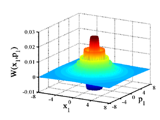
Figure 1: (Color online) The Wigner function of the reduced state of a $k$-photon two-mode squeezed vacuum state as represented in the phase space defined by $\hat{x}_{1}=\hat{a}_{1}^{\dagger}+\hat{a},\hat{p}_{1}=i(\hat{a}_{1}^{\dagger}-\hat{a}_{1})$ with $k=3$. This state is non-Gaussian.

In this paper we approach the problem from a different perspective. The Wigner function of the reduced state of a two-mode quantum state is shown in Fig. 1. Clearly the Wigner function is non-Gaussian and hence the two-mode state from which it is derived is non-Gaussian as well. Say an experimentalist measures (that is reconstructs from a tomographically complete measurement) this state in the laboratory. What exactly can she say about the separability of the state? At first sight not a great deal. However we will show that in fact this state’s separability is completely known and understood in terms of its interpretation as a Gaussian state. Furthermore we introduce a whole class of these states for which the usual two-mode Gaussian states are a special case.

Gaussian states of a two-mode continuous variable quantum system have been much studied in the literature and their entanglement properties are quite well established seraf ; dmmzvb . Here we briefly review their characterization. Let $\hat{a}^{\dagger},\hat{a}$ be the bosonic creation and annihilation operators acting on a Fock Hilbert space as $\hat{a}|\,n\rangle=\sqrt{n}|\,n-1\rangle$, $\hat{a}^{\dagger}|\,n\rangle=\sqrt{n+1}|\,n+1\rangle$ and satisfying the Weyl-Heisenberg commutation relations $[\hat{a},\hat{a}^{\dagger}]=1{\rm I}$. We can introduce position and momentum operators $\hat{x}=\hat{x}^{\dagger}+\hat{x}$, $\hat{p}=i(\hat{a}^{\dagger}-\hat{a})$ (setting $\hbar=1$) which define phase space through the continuous range of their eigenvalues. For two modes these position and momentum operators are defined in each Hilbert space. We gather these operators into a single vector $\vec{\hat{x}}=(\hat{x}_{1},\hat{p}_{1},\hat{x}_{2},\hat{p}_{2})$ for clarity. By definition the Wigner function of a Gaussian state, $\rho$, takes the form $W(x)=\exp[-x^{\prime}\sigma x^{\prime T}/2]/\pi\sqrt{\det\sigma}$, where $x^{\prime}=x-\langle\hat{x}\rangle$ and $\sigma_{jk}=(\langle\hat{x}_{j}\hat{x}_{k}+\hat{x}_{k}\hat{x}_{j}\rangle)/2-\langle\hat{x}_{j}\rangle\langle\hat{x}_{k}\rangle$ is called the covariance matrix with $\langle\hat{O}\rangle={\mbox{Tr}}[\rho\hat{O}]$. The Wigner function thus depends only on the first and second moments of the position and momentum operators marcinkiewicz . Furthermore, via local operations the covariance matrix can be brought to the simpler form

$$\sigma_{sf}=\left(\begin{array}[]{cccc}b_{1}&0&c_{1}&0\\ 0&b_{2}&0&c_{2}\\ c_{1}&0&d_{1}&0\\ 0&c_{2}&0&d_{2}\end{array}\right),$$ (1)

where $b_{i},c_{i}$ and $d_{i}$ satisfy $\frac{b_{1}-1}{d_{1}-1}=\frac{b_{2}-1}{d_{2}-1}$ and $\mid c_{1}\mid-\mid c_{2}\mid=\sqrt{(b_{1}-1)(d_{1}-1)}-\sqrt{(b_{2}-1)(d_{2}-1)}$ as shown in Ref. cirac . The necessary and sufficient condition for the state to be separable is then

$$\langle(\Delta\hat{u})^{2}\rangle+\langle(\Delta\hat{v})^{2}\rangle\geq q_{0}^{2}+\frac{1}{q_{0}^{2}},$$ (2)

with $\hat{u}=q_{0}\hat{x}_{1}-\frac{c_{1}}{\mid c_{1}\mid q_{0}}\hat{x}_{2}$, $\hat{v}=q_{0}\hat{p}_{1}-\frac{c_{2}}{\mid c_{2}\mid q_{0}}\hat{p}_{2},$ and $q_{0}^{2}=\sqrt{(d_{i}-1)/(b_{i}-1)}$. Actually this expression simplifies to $\sum_{j=1}^{2}\sqrt{(b_{j}-1)(d_{j}-1)}\geq\sum_{j=1}^{2}\mid c_{j}\mid$ when both $b_{1}-1\geq 0$ and $d_{1}-1\geq 0$ or $\sum_{j=1}^{2}(-1)^{j}\sqrt{(b_{j}-1)(d_{j}-1)}\geq\sum_{j=1}^{2}\mid c_{j}\mid$ otherwise. In the following section we impose an additional criterion: we will relate the degree of entanglement of Gaussian states to an energy of these states.

Gaussian states are an important class of states, but some quantum protocols require paris the usage of non-Gaussian states. These states are more difficult to handle mathematically than Gaussian states which only require knowledge of the first and second moments of a finite set of observables. One of the reasons why it is more difficult to analyse non-Gaussian states is that they are characterized by an infinite set of non-zero cumulants i.e. higher-order moments of system observables cannot be expressed in terms of the first and second order moments. What is important to note is that in order to define Gaussian states one needs to be able to construct observables from creation and annihilation operators which satisfy the Weyl-Heisenberg commutation relations. It is therefore possible to choose other operators satisfying these commutation relations and use these to construct new observables whose eigenvalues define a completely different phase space. In particular we can choose multi-photon operators like

$$\hat{A}^{(k)\dagger}=\sqrt{\left[\left[\frac{\hat{N}}{k}\right]\right]\frac{(\hat{N}-k)!}{\hat{N}!}}\hat{a}^{\dagger k},$$ (3)

as in Ref. brandt , satisfying $[\hat{A}^{(k)},\hat{A}^{(k)\dagger}]=1{\rm I}$ where $\hat{N}=\hat{a}^{\dagger}\hat{a}$, $[[\hat{N}/k]]=\sum_{n}[[n/k]]|\,n\rangle\langle n\,|$, $(\hat{N}-k)!/\hat{N}!=\sum_{n}\frac{(n-k)!}{n!}|\,n\rangle\langle n\,|$, and $[[n/k]]$ denotes the largest positive integer less than or equal to $n/k$ . They are constructed in such a way as to create or annihilate $k$ photons at a time. These operators can also be interpreted as acting on a “multi-photon Fock space”, $\tilde{\cal H}$, as $\hat{A}^{(k)\dagger}|\,n\rangle_{k}=\sqrt{n+1}|\,n+1\rangle_{k}$, $\hat{A^{(k)}}|\,n\rangle_{k}=\sqrt{n}|\,n-1\rangle_{k}$ where the subscript on the multi-photon number state $|\,n\rangle_{k}$ indicates we are referring to those states satisfying

$$|\,n\rangle_{k}=\frac{\hat{A}^{(k)\dagger n}}{\sqrt{n!}}|\,0\rangle_{k}.$$ (4)

Their action on the usual Fock space is given by

$$\hat{A}^{(k)\dagger}|\,nk+m\rangle = \sqrt{n+1}|\,(n+1)k+m\rangle$$

$$\hat{A}^{(k)}|\,nk+m\rangle = \sqrt{n}|\,(n-1)k+m\rangle,$$ (5)

with $n\geq 0$ and $0\leq m\leq k-1$. Thus, for the multiphoton number operators $\hat{N}^{(k)}=\hat{A}^{(k)^{\dagger}}\hat{A}^{(k)}$ each eigenvalue is k-times degenerated (including the vacua, i.e. $\hat{A}^{(k)}|\,m\rangle=0$ for $m<k$).

As before we can construct position and momentum operators (acting on $\tilde{\cal H}$ only) for the two modes $\vec{X}^{(k)}=(\hat{X}_{1}^{(k)},\hat{P}_{1}^{(k)},\hat{X}_{2}^{(k)},\hat{P}_{2}^{(k)})$ with $\hat{X}_{j}^{(k)}=\hat{A}_{j}^{(k)\dagger}+\hat{A}_{j}^{(k)}$, $\hat{P}_{j}^{(k)}=i(\hat{A}_{i}^{(k)\dagger}-\hat{A}_{j}^{(k)})$ and the eigenvalues of these operators define the phase space. In this phase space we have Gaussian states whose Wigner functions are Gaussian while if we represent the states using a Wigner function in the usual phase space the states are highly non-Gaussian. The separability criterion from Ref. cirac carries over here so that given a state has a covariance matrix in the form

$$\sigma_{sf}=\left(\begin{array}[]{cccc}B^{(k)}_{1}&0&C^{(k)}_{1}&0\\ 0&B^{(k)}_{2}&0&C^{(k)}_{2}\\ C^{(k)}_{1}&0&D^{(k)}_{1}&0\\ 0&C^{(k)}_{2}&0&D^{(k)}_{2}\end{array}\right),$$ (6)

we know it is separable if

$$\sum_{j=1}^{2}\sqrt{(B^{(k)}_{j}-1)(D^{(k)}_{j}-1)}\geq\sum_{j=1}^{2}\mid C^{(k)}_{j}\mid,$$ (7)

when both $B^{(k)}_{1}-1\geq 0$ and $D^{(k)}_{1}-1\geq 0$ or

$$\sum_{j=1}^{2}(-1)^{j}\sqrt{(B^{(k)}_{j}-1)(D^{(k)}_{j}-1)}\geq\sum_{j=1}^{2}\mid C^{(k)}_{j}\mid,$$ (8)

otherwise. Of course the local operations required to transform the state under consideration to one which can be represented by such a covariance matrix are non-Gaussian operations in terms of the creation and annihilation operators $\hat{a}_{1}^{\dagger},\hat{a}_{1},\hat{a}_{2}^{\dagger},\hat{a}_{2}$. Experimentally the operations could be constructed as proposed in Ref. braunlloyd .

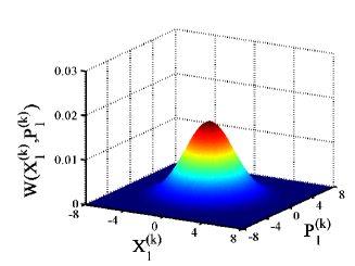
Figure 2: (Color online) The Wigner function of the reduced state of a $k$-photon two-mode squeezed vacuum state as represented in the phase space defined by $\hat{X}_{1}=\hat{A}_{1}^{(k)\dagger}+\hat{A}^{(k)},\hat{P}_{1}=i(\hat{A}_{1}^{(k)\dagger}-\hat{A}_{1}^{(k)})$ with $k=3$. The state is a thermal state and its Gaussian nature is clearly evident.

As an example we can take the multi-photon two-mode squeezed vacuum state which has the form $|\,\Psi\rangle=\sqrt{1-\gamma^{2}}\sum_{n}\gamma^{n}|\,n\rangle_{k}|\,n\rangle_{k}$. The reduced state in either mode is given by $\rho^{(k)}=(1-\gamma^{2})\sum_{n}\gamma^{2n}|\,n\rangle_{k}\langle n\,|$, a thermal state. The Wigner function of this state in the $(X^{(k)}_{1},P^{(k)}_{1})$ reduced phase space is shown in Fig. 2 and has the expected Gaussian form. However a simple calculation shows us that

$$|\,\Psi\rangle = \sqrt{1-\gamma^{2}}\sum_{n}\gamma^{n}\frac{\hat{A}_{1}^{(k)\dagger n}\hat{A}_{2}^{(k)\dagger n}}{n!}|\,0\rangle_{k}|\,0\rangle_{k}$$ (9)

$$= \sqrt{1-\gamma^{2}}\sum_{n}\gamma^{n}|\,kn\rangle|\,kn\rangle$$

giving a reduced density matrix $\rho=(1-\gamma^{2})\sum_{n}\gamma^{2n}|\,kn\rangle\langle kn\,|$. The Wigner function for this state in the $(x_{1},p_{1})$ reduced phase space is plotted in Fig. 1 showing that it is clearly non-Gaussian and even contains negative parts.

The covariance matrix of the two-mode multi-photon squeezed state is as in Eq. (6) with $B^{(k)}_{i}=D^{(k)}_{i}=\cosh 2r$ and $C^{(k)}_{1}=\sinh 2r=-C^{(k)}_{2}$ where $\gamma=\tanh r$. The separability criterion in Eq. (7) reads $\exp(-2r)\geq 1$ and the state is entangled for $r>0$. How then does the separability criterion relate to measurements of observables in the usual Fock space? For example we need to know what $B^{(k)}_{1}$ is and to this end we must measure $\langle\hat{X}^{(k)2}_{1}\rangle$ and $\langle\hat{X}^{(k)}_{1}\rangle$. For the case $k=2$ we find these expectation values in terms of the operators $\hat{a}_{1},\hat{a}^{\dagger}_{1}$ are

$$\langle\hat{X}_{1}^{(k)\dagger 2}\rangle = \frac{1}{2}\left(\left\langle\sqrt{\frac{1}{(\hat{N}_{1}+1)(\hat{N}_{1}+3)}}\hat{a}_{1}^{4}\right\rangle\right.$$

$$+ \left.\left\langle\hat{a}_{1}^{\dagger 4}\sqrt{\frac{1}{(\hat{N}_{1}+1)(\hat{N}_{1}+3)}}\right\rangle+2\langle\hat{N}_{1}\rangle+21{\rm I}\right)$$

and

$$\langle\hat{X}^{(k)}_{1}\rangle^{2}=\frac{1}{2}\left(\left\langle\sqrt{\frac{1}{\hat{N}_{1}+1}}\hat{a}_{1}^{2}\right\rangle+\left\langle\hat{a}_{1}^{\dagger 2}\sqrt{\frac{1}{\hat{N}_{1}+1}}\right\rangle\right)^{2}$$ (11)

with $\hat{N}_{1}=\hat{a}^{\dagger}_{1}\hat{a}_{1}$. While we readily concede that it is a non-trivial task to experimentally measure these expectation values we are motivated by what one is able to say about the separability of a state when full tomography has been carried out and the result is a state such as that in Fig. 1.

For a given squeezing parameter $\gamma$ the two-mode squeezed vacuum state $|\,\Phi\rangle=\sqrt{1-\gamma^{2}}\sum_{n}\gamma^{n}|\,n,n\rangle$ and its multi-photon equivalent $|\,\Psi\rangle=\sqrt{1-\gamma^{2}}\sum_{n}\gamma^{n}|\,n,n\rangle_{k}$ will posess the same degree of entanglement, a fact most easily seen using the the von Neumann entropy of the reduced state of either mode, $S=-{\mbox{Tr}}\rho_{1}\ln\rho_{1}=-{\mbox{Tr}}\rho^{(k)}_{1}\ln\rho^{(k)}_{1}=S^{(k)}$. It should be noted however that uncovering the two-mode entanglement present in each of the above states requires measurement of different observables. In what follows we will compare two states of a two-mode system at a fixed energy value dmmzvb . In terms of the average energy $\langle E\rangle\equiv\langle\Phi\,|\sum_{i}\hat{N}_{i}|\,\Phi\rangle$ with $\hat{N}_{i}=\hat{a}^{\dagger}_{i}\hat{a}_{i}$ the multi-photon squeezed vacuum state with the same degree of entanglement has average energy $\langle E^{(k)}\rangle=k\langle E\rangle$. If we fix the energy of both states at $\langle E\rangle=2\bar{n}$ where $\bar{n}=\langle\Phi\,|N_{i}|\,\Phi\rangle$ then the reduced state of $|\,\Phi\rangle$ can be written as $\rho_{1}=\sum_{n}p_{n}|\,n\rangle\langle n\,|$ with $p_{n}=\bar{n}^{n}/(1+\bar{n})^{1+n}$ and the reduced state of $|\,\Psi\rangle$ can be similarly written as $\rho_{1}^{(k)}=\sum_{n}p_{n}^{(k)}|\,n\rangle_{k}\langle n\,|$ with $p_{n}^{(k)}=\left(\frac{\bar{n}}{k}\right)^{n}/(1+\frac{\bar{n}}{k})^{1+n}$. Thus it is clear that for fixed energy the usual two-mode squeezed vacuum is more entangled than its multi-photon counterpart. Intuitively this makes sense given that the nature of the multi-photon state does not allow certain quantum correlations to exist; for instance, upon measurement of the state in the joint number basis there is zero probability to obtain the result $|\,kn+m,kn+m\rangle$ for $m<k$ and $n\in\mathbb{Z}^{+}$. This result also ties in with the fact that among all continuous variable states with a given fixed energy, the maximally entangled states are Gaussian wolfy .

For mixed states we compare a $k$-photon two-mode mixed state with a usual two-mode mixed state having the same average energy $\langle E\rangle$. To get an intuitive sense of the difference between two such states we look for the minimum purity (defined as $P(\omega)={\rm Tr}\omega^{2}$) allowed for the $k$-photon mixed state given this energy $\langle E\rangle$. The dependence on $k$ is

$$P^{(k)}_{min}=\frac{1}{(\frac{\langle E\rangle}{k}+1)^{2}},$$ (12)

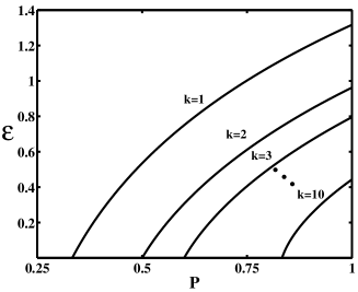
Figure 3: The maximally entangled mixed states of the multi-photon Gaussian states plotted at the same average energy $\langle E\rangle=1$ (units are dimensionless) for different values of $k$. The log-negativity, $\mathcal{E}$, is used to measure the entanglement while the purity, $P$, is used to indicate how mixed the state is.

corresponding to a tensor product of two multi-photon thermal states. As $k$ increases the minimum purity increases asymptotically toward 1 so that the $k$-photon mixed states tend toward the vacuum in the limit $k\rightarrow\infty$. To re-enforce this point in Fig. 3 we plot the maximally entangled multi-photon Gaussian mixed states, see Ref. dmmzvb , for various values of $k$, all at a fixed mean energy $\langle E\rangle=1$. Thus we can say that the maximally entangled $k$-photon mixed states are less entangled than those for $k=1$. For general mixed states this statement is not always true.

We have presented a large class of non-Gaussian states for which the existing separability criterion for Gaussian states can be employed in order to detect their entanglement. In order to clarify our results we recall that an arbitrary unitary transformation $U:{\cal H}\to{\cal H}$ resulting in an “annihilation” operator $\hat{b}_{U}=U\hat{a}U^{\dagger}$ can be exploited to define another class of non-Gaussian states ${\cal C}_{U}=\{\varrho:\varrho=U^{\dagger}\tilde{\varrho}U,\tilde{\varrho}\in{\cal G}\}$, where $\cal G$ denotes the set of “standard” Gaussian states. Due to the fact that unitary transformations preserve an operator’s spectra and the commutation relations, the operators $\hat{b}_{U},\hat{b}^{\dagger}_{U}$ form a representation of the Weyl-Heisenberg group and Gaussian states with respect to these operators can be defined. In fact, as it was pointed out in Ref. cirac the inequality in Eq.(2) provides a sufficient separability criterion for all operators $\hat{\mu},\hat{\nu}$ that are locally unitary equivalent to $\hat{u},\hat{v}$, i.e. $\hat{\mu}=U\hat{u}U^{\dagger}$, $\hat{\nu}=U\hat{v}U^{\dagger}$, respectively. Moreover, these inequalities provide the necessary conditions for entanglement for all Gaussian states defined with respect to new phase-space coordinates, i.e. for all $\varrho\in{\cal C}_{U}$.

We have to note that even though the multi-photon non-Gaussian states analyzed in our paper seem to be of the similar form as discussed above, there is a significant difference. The operators $\hat{a}$ and $\hat{A}_{k}$ are not mutually related by a unitary transformation in the above sense (for more details see Ref. luis93 ). In fact, the number operators $\hat{N}_{k}$ and $\hat{n}$ have different spectra ($\hat{N}_{k}$ is degenerated). The construction in our case is based on the fact that the (semi)infinite Hilbert space of the original harmonic oscillator can be expressed as a finite direct sum of (semi)infinite Hilbert spaces that are isomorphic to the original one, i.e. ${\cal H}=\tilde{\cal H}_{0}\oplus\cdots\oplus\tilde{\cal H}_{k-1}$. Here $\tilde{\cal H}_{j}$ is a linear span of vectors ${\cal H}\ni|\,nk+j\rangle\equiv|\,n\rangle_{j,k}\in\tilde{\cal H}_{j}$ ($n=0,\dots,\infty$). Physically this means that we are restricted to states belonging to the subspace spanned on photon number states separated by a fixed energy $k\hbar\omega$ (representing the energy of $k$ photons). The vacuum for $\tilde{\cal H}_{j}$ is represented by the state $|\,0+j\rangle=|\,j\rangle\in{\cal H}$ The linear spaces ${\cal H}$ and $\tilde{\cal H}_{j}$ are related by a non-bijective transformation. However, since $\tilde{H}_{j}$ and $\tilde{\cal H}_{j^{\prime}}$ are in one-to-one correspondence, we can write ${\cal H}=\bigoplus_{j=0}^{k-1}\tilde{\cal H}_{j}=\tilde{\cal H}_{k}\otimes{\cal V}_{k}$ (${\rm dim}\tilde{\cal H}_{k}=\infty$ and ${\rm dim}{\cal V}_{k}=k$). Using this notation the multiphoton annihilation operators are unitarily related to the original annihilation operator (acting on $\tilde{\cal H}_{k}$) via the unitary transformation $\tilde{U}=\sum_{n,m}(|\,n\rangle_{k}\otimes|\,m\rangle)\langle kn+m\,|$ luis93 performing the transformation from ${\cal H}$ to $\tilde{\cal H}_{k}\otimes{\cal V}_{k}$. In particular, $\tilde{U}\hat{A}^{(k)}\tilde{U}^{\dagger}=\tilde{a}\otimes I$.

The Gaussian states are naturally a special case of these non-Gaussian states as one would expect. For two modes the operation moving from the basis in which the states have a Gaussian Wigner representation to that in which they don’t is local unitary and as such preserves the entanglement. This holds for $\hat{b}_{U}$, but also for multiphoton operators $\hat{A}^{(k)}$, hence the criterion derived for standard Gaussian states can be directly applied to multiphoton Gaussian states as it was demonstrated in the present work. A question remains is how to efficiently verify whether a given state belongs to a certain sector of the Hilbert space $\tilde{\cal H}_{j}$ for a given $k$, or not. The answer can be given by analyzing the expression for the state under consideration in the Fock basis. If the populated (i.e. non-vanishing) levels are separated by the same energy (equivalently, by the same number of photons), then the state belongs to a multiphoton sector $\tilde{\cal H}$ of the Hilbert space $\cal H$ and its multiphoton Wigner function can be further analyzed.

Acknowledgement
This work was supported in part by the European Union projects INTAS-04-77-7289, CONQUEST and QAP, by the Slovak Academy of Sciences via the project CE-PI/2/2005, by the project APVT-99-012304.

References

(1) C. H. Bennett et al.,
Phys. Rev. Lett. 70, 1895 (1993);
S. L. Braunstein et al., Phys. Rev. Lett. 80, 869 (1998).
(2) C. H. Bennett et al.,
Proc. of IEEE International Conference on Computers, Systems and Signal
Processing, Bangalore, India (IEEE, New York, 1984), p. 175; M.
Hillery, Phys. Rev. A 61, 022309 (2000).
(3) A. Peres, Phys. Rev. Lett. 77, 1413 (1996).
(4) P. van Loock, Fort. der Phys. 50, 1177
(2002).
(5) R. Simon, Phys. Rev. Lett. 84, 2726 (2001).
(6) L. M. Duan et al.,
Phys. Rev. Lett. 84, 2722 (2001).
(7) E. Schukin et al., Phys. Rev. Lett. 95, 230502 (2005); E. Schukin et al., Phys. Rev. A 74, 030302(R) (2006).
(8) A. Miranowicz et al., quant-ph/0605001.
(9) G. S. Agarwal and A. Biswas, New J. Phys. 7,
211 (2005).
(10) M. Hillery et al.,
Phys. Rev. Lett. 96, 050503 (2006).
(11) H. Nha and J. Kim, Phys. Rev. A 74, 012317
(2006).
(12) G. Adesso et al.,
Phys. Rev. Lett. 92, 087901 (2004); G. Adesso et al.,
Phys. Rev. A 70, 022318 (2004).
(13) D. McHugh et al.,
Phys. Rev. A 74, 042303 (2006).
(14) J.Marcinkiewicz, Math. Z. 44, 612 (1939).
(15) S. Olivares et al.,
Phys. Rev. A 70, 032112 (2004).
(16) R. A. Brandt et al.,
J. Math. Phys. 10, 1168 (1969).
(17) S. Lloyd et al.,
Phys. Rev. Lett. 82, 1784 (1999).
(18) M. M. Wolf et al.,
Phys. Rev. Lett. 96, 080802 (2006).