Electron Fabry-Perot interferometer with two entangled magnetic impurities

Abstract

We consider a one-dimensional (1D) wire along which single conduction electrons can propagate in the presence of two spin-1/2 magnetic impurities. The electron may be scattered by each impurity via a contact-exchange interaction and thus a spin-flip generally occurs at each scattering event. Adopting a quantum waveguide theory approach, we derive the stationary states of the system at all orders in the electron-impurity exchange coupling constant. This allows us to investigate electron transmission for arbitrary initial states of the two impurity spins. We show that for suitable electron wave vectors, the triplet and singlet maximally entangled spin states of the impurities can respectively largely inhibit the electron transport or make the wire completely transparent for any electron spin state. In the latter case, a resonance condition can always be found, representing an anomalous behaviour compared to typical decoherence induced by magnetic impurities. We provide an explanation for these phenomena in terms of the Hamiltonian symmetries. Finally, a scheme to generate maximally entangled spin states of the two impurities via electron scattering is proposed.

1 Introduction

The remarkable recent progress in the fabrication techniques of nanometric semiconductor structures has stimulated a rapid development of the emerging field of mesoscopic physics [1, 2, 3]. In particular, the fabrication of devices of a size shorter than the electron coherence length has motivated the study of systems where the conduction electrons exhibit a fully quantum mechanical behaviour. Such systems are the electron analogue of optical devices. For instance, a multichannel quantum wire can be regarded as the electron counterpart of an electromagnetic waveguide [3].

On the other hand, there is an active research on the coherent dynamics of the electron spin in mesoscopic systems [4] due to its potential applications to the control of electron transport in so-called “spintronic” devices [5], as well as in the implementations of quantum information processing devices [6]. Such interest is justified by the long decoherence times/distances exhibited by electron spin in semiconductors [4].

In this paper, we consider a 1D wire with two spin-1/2 magnetic impurities embedded at fixed positions. The 1D wire could be realized by a semiconductor quantum wire [2] or a single-wall carbon nanotube [7], while each impurity could be implemented by means of a single-electron quantum dot [4]. Conduction electrons entering the wire undergo multiple scattering by the two impurities before being reflected or transmitted. At each scattering event the electron and impurity spins elastically interact via an exchange coupling which can induce a spin-flip. If the two impurities were static, the present system would reduce to the electron analogue of a Fabry-Perot (FP) interferometer with partially silvered mirrors [8], with the impurities playing the role of the two mirrors. It follows that our system can be considered as a generalized FP interferometer where each mirror has a quantum degree of freedom: the spin.

Since scattering with magnetic impurities is a well-known source of electron decoherence [3], one would expect that, when mirrors with internal degrees of freedom are considered, the typical resonance condition found in a standard FP interferometer [8] would be modified. The expected loss of electron coherence is due to the fact that – contrary to scattering by static impurities which give rise to well fixed phase-shifts – scattering by magnetic impurities causes an uncertainty in the phase shift of the scattered electron [9, 10]. Equivalently, decoherence can be regarded as a consequence of the unavoidable entanglement arising between the electron and impurity spin degrees of freedom [9, 11].

In the present paper, we analyze the case where two magnetic impurities are embedded in the wire. In [12] we have investigated how non-local correlations arising when the scatterers are in an entangled state affect the wire transmittivity. In the present paper, we will extend our analysis providing all the details of our approach and expand the discussion of the possible applications. In particular, we will show that perfect resonance, i.e. perfect transmittivity for suitable electron wave vectors, appears for the singlet maximally entangled state of the impurity spins. Remarkably, these resonant wave vectors turn out to be independent on the electron-impurity coupling constant. Moreover, when this resonant condition is fulfilled, perfect transmittivity is obtained for all possible electron spin states. On the contrary, a large inhibition of electron transmission through the interferometer is observed for the case of the triplet maximally entangled state. As we have pointed out in a recent work, the above behaviour of the singlet and triplet entangled states suggests a novel potential use of entanglement as a tool to modulate the conductance of a 1D wire [12].

This paper is organized as follows. In section 2, we describe in detail the system and the approach used to derive all the transmission amplitudes needed to calculate the single electron transmittivity for any arbitrary initial spin state. In section 3, we discuss the transmission properties of the interferometer for initial spin states with only one impurity spin up. Perfect “transparency” is exhibited for the singlet state of the impurities. Section 4 is devoted to the explanation of this phenomenon. In section 5, we show how our results suggest a possible use of entanglement of the impurity spins as a tool to modulate the transmission of the wire. In section 6 we investigate the transmission properties of a different family of impurity spin states, namely the one for which both spins are aligned. We show that, in this case, entangled states exhibit no relevant interference effects. Finally, in section 7 we propose a scheme to generate maximally entangled states of the impurity spins via electron scattering. The form that an initial spin state must have in order to have perfect transparency is derived in A.

2 System and approach

Our system consists of a clean 1D wire into which two spatially separated, identical spin-1/2 magnetic impurities are embedded. We assume that single conduction electrons can be injected into the wire. Due to the presence of an exchange interaction, each conduction electron undergoes multiple scattering with the impurities before being transmitted or reflected. Let us also assume that the electron spin state can be prepared at the input of the wire and measured at its output (this could be achieved through ferromagnetic contacts at the source and drain of the wire [4]). To be more specific, consider a 1D wire along the $\hat{x}$ direction with the two magnetic impurities, labeled 1 and 2, embedded at $x=0$ and $x=x_{0}$, respectively, as illustrated in figure 1.

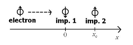
Figure 1: 1D wire with two magnetic impurities, labeled 1 and 2, embedded at $x=0$ and $x=x_{0}$, respectively.

Assuming that the conduction electrons are injected one at a time (this allows us to neglect many-body effects) and that they can occupy only the lowest subband, the Hamiltonian can be written as

$$H=\frac{p^{2}}{2m^{*}}+J\,\mbox{\boldmath$\sigma$}\cdot\mathbf{S}_{1}\,\delta(x)+J\,\mbox{\boldmath$\sigma$}\cdot\mathbf{S}_{2}\,\delta(x-x_{0})$$ (1)

where $p=-i\hbar\nabla$, $m^{*}$ and $\bm{\sigma}$ are the electron momentum operator, effective mass and spin-1/2 operator respectively, $\mathbf{S}_{i}$ ($i=1,2$) is the spin-1/2 operator of the $i$-th impurity and $J$ is the exchange spin-spin coupling constant between the electron and each impurity. All the spin operators are in units of $\hbar$. Since the electron-impurity collisions are elastic, the energy eigenvalues are simply $E=\hbar^{2}k^{2}/2m^{*}$ ($k>0$) where $k$ is a good quantum number. As the total spin Hilbert space is 8D and considering left-incident electrons, it turns out that to each value of $k$ there corresponds an 8-fold degenerate energy level. Let $\mathbf{S}=\bm{\sigma}+\mathbf{S}_{1}+\mathbf{S}_{2}$ be the total spin of the system. Since $\mathbf{S^{2}}$ and $S_{z}$, with quantum numbers $s$ and $m_{s}$, respectively, are constants of motion, $H$ can be block diagonalized, each block corresponding to an eigenspace of fixed $s$ (for three spins 1/2, the possible values of $s$ are $1/2,3/2$) and $m_{s}=-s,...,s$ (from now on the subscript $s$ in $m_{s}$ will be omitted). Let us rewrite equation (1) in the form

$$H=\frac{p^{2}}{2m^{*}}+\frac{J}{2}\left(\mathbf{S}_{e1}^{2}-\frac{3}{2}\right)\delta(x)+\frac{J}{2}\left(\mathbf{S}_{e2}^{2}-\frac{3}{2}\right)\delta(x-x_{0})$$ (2)

where $\mathbf{S}_{ei}=\bm{\sigma}+\mathbf{S}_{i}$ ($i=1,2$) is the total spin of the electron and the $i$-th impurity. Note that in general $\mathbf{S}_{e1}^{2}$ and $\mathbf{S}_{e2}^{2}$ do not commute.

Here we choose as spin space basis the states $\left|s_{e2};s,m\right\rangle$, common eigenstates of $\mathbf{S}_{e2}^{2}$, $\mathbf{S}^{2}$ and $S_{z}$ [13], to express, for a fixed $k$, each of the eight stationary states of the system as an 8D column. Since $\mathbf{S}_{e1}^{2}$ and $\mathbf{S}_{e2}^{2}$ do not commute, the latter in general is not a constant of motion and thus $s_{e2}$ in general is not a good quantum number.

To determine the transmission properties of the interferometer for a given arbitrary initial spin state, we have to calculate the transmission probability amplitudes $t_{s_{e2}}^{(s^{\prime}_{e2};s)}$ that an electron prepared in the incoming state $\left|k\right\rangle\left|s^{\prime}_{e2};s,m\right\rangle$ is transmitted in the state $\left|k\right\rangle\left|s_{e2};s,m\right\rangle$. The calculation of $t_{s_{e2}}^{(s^{\prime}_{e2};s)}$ requires the exact stationary states of the system to be derived. To do this, we properly generalize the quantum waveguide theory approach of reference [14] for an electron scattering with a single magnetic impurity to the case of two impurities. Note that due to the form of $H$ (see equation 2) coefficients $t_{s_{e2}}^{(s^{\prime}_{e2};s)}$ do not depend on $m$, as it will be more clear in the following. We first consider the subspace $s=3/2$ and then the subspace $s=1/2$.

2.1 Subspace $s=3/2$

In this 4D subspace ($m=-3/2,-1/2,1/2,3/2$), both $s_{e1}$ and $s_{e2}$ can assume only the value 1. It follows that in this subspace $\mathbf{S}_{e1}^{2}$ and $\mathbf{S}_{e2}^{2}$ effectively commute. The states $\left|s_{e2};s,m\right\rangle=\left|1;3/2,m\right\rangle$ are thus also eigenstates of $\mathbf{S}_{e1}^{2}$ and the effective electron-impurities potential $V$ in equation (2) reduces to

$$V=\frac{J}{4}\,\delta(x)+\frac{J}{4}\,\delta(x-x_{0})$$ (3)

Note that the two impurities behave as if they were static and the scattering between electron and impurities cannot flip the spins. The four stationary states take therefore the simple product form

$$\left|\Psi_{k,1;3/2,m}\right\rangle=\left|\phi_{k}\right\rangle\left|1;3/2,m\right\rangle$$ (4)

where the second index in the left-hand side stand for $s_{e2}=1$ and where $\left|\phi_{k}\right\rangle$ describes the electron orbital degrees of freedom. To determine the wave function $\phi_{k}(x)$, we split the $\hat{x}$ axis into the three domains $x<0$, $0<x<x_{0}$ and $x>x_{0}$ labeled I, II and III, respectively. Solving the Schrödinger equation, the wave function $\phi_{k,i}(x)$ in each domain $i=I,II,III$ is readily written as

$$\phi_{k,I}(x) = A_{I}e^{ikx}+B_{I}e^{-ikx}\$$ (5)

$$\phi_{k,II}(x) = A_{II}e^{ikx}+B_{II}e^{-ikx}$$ (6)

$$\phi_{k,III}(x) = t_{1}^{(1;3/2)}e^{ikx}$$ (7)

Setting $A_{I}$ to unity, the other four coefficients appearing in equations (5) – (7) can be found by requiring the wave function to be continuous at the two boundaries $x=0$ and $x=x_{0}$ and its derivative $\phi^{\prime}_{k}(x)$ to exhibit a jump at the same points according to

$$\phi^{\prime+}_{k}(0)-\phi^{\prime-}_{k}(0) = \frac{2m^{*}}{\hbar^{2}}\frac{J}{4}\,\phi_{k}(0)$$ (8)

$$\phi^{\prime+}_{k}(x_{0})-\phi^{\prime-}_{k}(x_{0}) = \frac{2m^{*}}{\hbar^{2}}\frac{J}{4}\,\phi_{k}(x_{0})$$ (9)

The last conditions are easily found integrating the Schrödinger equation across each impurity (see e.g. [15]). This yields the following result for the transmission amplitude $t_{1}^{(1;3/2)}$

$$t_{1}^{(1;3/2)}=\frac{64}{64+\pi\rho(E)J\,[16i+(e^{2ikx_{0}}-1)\rho(E)J]}$$ (10)

where $\rho(E)=(\sqrt{2m^{*}/E})/\pi\hbar$ is the density of states per unit length of the wire [1, 2]. $t_{1}^{(1;3/2)}$ is thus a function of the two dimensionless parameters $kx_{0}$ and $\rho(E)J$. Note that it does not depend on $m$ due to the effective form (3) of $V$.

2.2 Subspace $s=1/2$

In this 4D subspace $s_{e1},s_{e2}=0,1$ and thus $\mathbf{S}_{e1}^{2}$ and $\mathbf{S}_{e2}^{2}$ do not commute and $s_{e2}$ is not a good quantum number. This is a signature of the fact that in this space spin-flip may occur. In each of the 2D $m=-1/2,1/2$ subspaces, the two stationary states are thus of the form

$$\left|\Psi_{k,s_{e2}^{\prime};1/2,m}\right\rangle=\sum_{s_{e2}=0,1}\left|\varphi_{k,s_{e2}^{\prime},s_{e2}}\right\rangle\left|s_{e2};1/2,m\right\rangle$$ (11)

where we have used the labeling index $s_{e2}^{\prime}=0,1$ to indicate that the incident spin state of (11) is $\left|s_{e2}^{\prime};1/2,m\right\rangle$ and where $\left|\varphi_{k,s_{e2}^{\prime},s_{e2}}\right\rangle$ describe the electron orbital degrees of freedom (from now on we omit the index $k$). Note that in the case $s=3/2$ discussed in subsection 2.1 $s^{\prime}_{e2}$ and $s_{e2}$ coincide.

For a fixed $s^{\prime}_{e2}=0,1$ the two wave functions $\varphi_{s^{\prime}_{e2},0}(x)$ and $\varphi_{s^{\prime}_{e2},1}(x)$ in each domain $i=I,II,III$ turn out to take a form analogous to (5) – (7)

$$\varphi_{s^{\prime}_{e2},s_{e2},I}(x) = A_{s_{e2},\,I}^{(s^{\prime}_{e2})}\,e^{ikx}+B_{s_{e2},\,I}^{(s^{\prime}_{e2})}\,e^{-ikx}$$ (12)

$$\varphi_{s^{\prime}_{e2},s_{e2},II}(x) = A_{s_{e2},\,II}^{(s^{\prime}_{e2})}\,e^{ikx}+B_{s_{e2},\,II}^{(s^{\prime}_{e2})}\,e^{-ikx}$$ (13)

$$\varphi_{s^{\prime}_{e2},s_{e2},III}(x) = t_{s_{e2}}^{(s^{\prime}_{e2};1/2)}\,e^{ikx}$$ (14)

with $s_{e2}=0,1$. According to the above definition of $s^{\prime}_{e2}$, the stationary state corresponding to a given $s^{\prime}_{e2}$ is obtained by setting $A_{0,\,I}^{(s^{\prime}_{e2}=0)}=1$, $A_{1,\,I}^{(s^{\prime}_{e2}=0)}=0$ and $A_{0,\,I}^{(s^{\prime}_{e2}=1)}=0$, $A_{1,\,I}^{(s^{\prime}_{e2}=1)}=1$. In each case, one has to determine the remaining eight coefficients $B_{0,\,I}^{(s^{\prime}_{e2})},A_{0,\,II}^{(s^{\prime}_{e2})},B_{0\,,II}^{(s^{\prime}_{e2})},t_{0}^{(s^{\prime}_{e2};1/2)},B_{1,\,I}^{(s^{\prime}_{e2})},A_{1,\,II}^{(s^{\prime}_{e2})},B_{1\,,II}^{(s^{\prime}_{e2})},t_{1}^{(s^{\prime}_{e2};1/2)}$. To do this, we need eight constrains. Four of these are obtained imposing the continuity of both $\varphi_{s^{\prime}_{e2},0}(x)$ and $\varphi_{s^{\prime}_{e2},1}(x)$ at $x=0$ and $x=x_{0}$. The other four constrains come from appropriate boundary conditions for the derivatives of $\varphi_{s^{\prime}_{e2},0}(x)$ and $\varphi_{s^{\prime}_{e2},1}(x)$ at the impurities’ sites. To derive these, we insert the ansatz (11) into the Schrödinger equation

$$\Biggl{\{}\frac{p^{2}}{2m^{*}}+\frac{J}{2}\left(\mathbf{S}_{e1}^{2}-\frac{3}{2}\right)\delta(x)+\frac{J}{2}\left(\mathbf{S}_{e2}^{2}-\frac{3}{2}\right)\delta(x-x_{0})-E\Biggl{\}}\sum_{s_{e2}=0,1}\left|\varphi_{s_{e2}^{\prime},s_{e2}}\right\rangle\left|s_{e2};1/2,m\right\rangle=0$$

We now project both sides of equation (2.2) onto $\left|0;1/2,m\right\rangle$ and $\left|1;1/2,m\right\rangle$. This yields the two equations

$$\left\{-\frac{\hbar^{2}}{2m^{*}}\frac{d^{2}}{dx^{2}}+\frac{J}{2}\,\left[\langle 0\left|\mathbf{S}_{e1}^{2}\right|0\rangle-\frac{3}{2}\right]\delta(x)-\frac{3J}{4}\,\delta(x-x_{0})-\frac{\hbar^{2}k^{2}}{2m}\right\}\left|\varphi_{s_{e2}^{\prime},0}\right\rangle$$

$$+\frac{J}{2}\langle 1\left|\mathbf{S}_{e1}^{2}\right|0\rangle\,\delta(x)\left|\varphi_{s_{e2}^{\prime},1}\right\rangle=0$$ (16)

$$\left\{-\frac{\hbar^{2}}{2m^{*}}\frac{d^{2}}{dx^{2}}+\frac{J}{2}\left[\,\langle 1\left|\mathbf{S}_{e1}^{2}\right|1\rangle-\frac{3}{2}\right]\delta(x)+\frac{J}{4}\,\delta(x-x_{0})-\frac{\hbar^{2}k^{2}}{2m}\right\}\left|\varphi_{s_{e2}^{\prime},1}\right\rangle$$

$$+\frac{J}{2}\langle 1\left|\mathbf{S}_{e1}^{2}\right|0\rangle\,\delta(x)\left|\varphi_{s_{e2}^{\prime},0}\right\rangle=0$$ (17)

where $\left|0\right\rangle$ and $\left|1\right\rangle$ stand for $\left|0;1/2,m\right\rangle$ and $\left|1;1/2,m\right\rangle$, respectively. The matrix elements of $\mathbf{S}_{e1}^{2}$ appearing in (16) – (17) can be computed through a change of the coupling scheme expressing basis states $\left|s_{e2};1/2,m\right\rangle$ in terms of $\left|s_{e1};1/2,m\right\rangle$ by means of $6j$ coefficients. This yields

$$\langle 0\left|\mathbf{S}_{e1}^{2}\right|0\rangle=\frac{3}{2}\,\,\,\,\,\,\,\,\,\,\,\langle 1\left|\mathbf{S}_{e1}^{2}\right|0\rangle=\langle 0\left|\mathbf{S}_{e1}^{2}\right|1\rangle=\frac{\sqrt{3}}{2}\,\,\,\,\,\,\,\,\,\,\langle 1\left|\mathbf{S}_{e1}^{2}\right|1\rangle=\frac{1}{2}$$ (18)

Using (18) and integrating both equations (16) and (17) across $x=0$ and $x=x_{0}$, we end with the four equations

$$\Delta\varphi_{s_{e2}^{\prime},0}^{\prime}(0)=\frac{2m^{*}J}{\hbar^{2}}\frac{\sqrt{3}}{4}\,\varphi_{s_{e2}^{\prime},1}(0)$$ (19)

$$\Delta\varphi_{s_{e2}^{\prime},1}^{\prime}(0)=-\frac{2m^{*}J}{\hbar^{2}}\frac{1}{2}\,\varphi_{s_{e2}^{\prime},1}(0)+\frac{2m^{*}J}{\hbar^{2}}\frac{\sqrt{3}}{4}\,\varphi_{s_{e2}^{\prime},0}(0)$$ (20)

$$\Delta\varphi_{s_{e2}^{\prime},0}^{\prime}(x_{0})=-\frac{2m^{*}J}{\hbar^{2}}\frac{3}{4}\,\varphi_{s_{e2}^{\prime},0}(x_{0})$$ (21)

$$\Delta\varphi_{s_{e2}^{\prime},1}^{\prime}(x_{0})=\frac{2m^{*}J}{\hbar^{2}}\,\frac{1}{4}\,\varphi_{s_{e2}^{\prime},1}(x_{0})$$ (22)

where $\Delta\varphi^{\prime}_{s_{e2}^{\prime},s_{e2}}(x)=\varphi_{s_{e2}^{\prime},s_{e2}}^{{}^{\prime}+}(x)-\varphi_{s_{e2}^{\prime},s_{e2}}^{{}^{\prime}-}(x)$.

Equations (19) – (22) represent the appropriate boundary conditions for the derivatives of $\varphi_{s^{\prime}_{e2},0}(x)$ and $\varphi_{s^{\prime}_{e2},1}(x)$ at the impurities’ sites. Note that these imply a coupling between $\left|\varphi_{s^{\prime}_{e2},0}\right\rangle$ and $\left|\varphi_{s^{\prime}_{e2},1}\right\rangle$, as witnessed by equations (19) and (20) and ultimately by the terms proportional to $\langle 1\left|\mathbf{S}_{e1}^{2}\right|0\rangle$ appearing in (16) and (17). This coupling thus results from non commutation of $\mathbf{S}_{e1}^{2}$ and $\mathbf{S}_{e2}^{2}$.

As equations (19) – (22) are added to the matching conditions of $\varphi_{s^{\prime}_{e2},0}(x)$ and $\varphi_{s^{\prime}_{e2},1}(x)$ at $x=0$ and $x=x_{0}$ a linear system of 8 equations is obtained. Once this is solved for $s^{\prime}_{e2}=0$ and $s^{\prime}_{e2}=1$, the following transmission amplitudes $t_{s_{e2}}^{(s^{\prime}_{e2};1/2)}$ are obtained

$$t^{(s_{e2}^{\prime};1/2)}_{0} = \frac{1}{\delta}\left[-64\,e^{2ikx_{0}}\pi^{2}(\rho(E)J)^{2}\left(2(1-s_{e2}^{\prime})+\sqrt{3}s_{e2}^{\prime}\right)\right.$$

$$+ \left.64(\pi\rho(E)J-8i)\left(2(4i+\pi\rho(E)J)(1-s_{e2}^{\prime})+\sqrt{3}\pi\rho(E)Js_{e2}^{\prime}\right)\right]$$

$$t^{(s_{e2}^{\prime};1/2)}_{1} = \frac{64}{\delta}\left[\sqrt{3}\pi\rho(E)J\left(-8i+3(e^{2ikx_{0}}-1)\pi\rho(E)J\right)(1-s_{e2}^{\prime})\right.$$

$$+ \left.\,8s_{e2}^{\prime}(8-3i\pi\rho(E)J)\right]$$

with

$$\delta = \left\{4096+\pi\rho(E)J\left[-2048i+\left(e^{2ikx_{0}}-1\right)\pi\rho(E)J\right.\right.$$ (25)

$$\times \left.\left.\left(-128+96i\pi\rho(E)J+9\left(e^{2ikx_{0}}-1\right)\pi^{2}(\rho(E)J)^{2}\right)\right]\right\}$$

As in the case $s=3/2$, the coefficients $t_{s_{e2}}^{(s^{\prime}_{e2};1/2)}$ are functions of $kx_{0}$ and $\rho(E)J$ and, moreover, they again do not depend on $m$ as suggested by the notation here adopted. The latter circumstance is due to the form (2) of $H$ and to the fact that $6j$ coefficients – and thus matrix elements (18) appearing in (16), (17) – do not depend on $m$ (see e.g. [20]).

As a further signature of non conservation of $\mathbf{S}_{e2}^{2}$ in the present subspace note that $t^{(s_{e2}^{\prime};1/2)}_{s_{e2}}\neq 0$ for $s_{e2}\neq s_{e2}^{\prime}$.

2.3 Calculation of transmittivity for an arbitrary spin state

It is important to stress again that our calculated transmission amplitudes $t^{(s_{e2}^{\prime};1/2)}_{s_{e2}}$ are exact at all orders in the electron-impurity coupling constant $J$. This follows from our quantum waveguide theory approach which addresses the determination of the stationary states through resolution of the Schrödinger equation. This approach is different from the perturbative one adopted in [17] where only a finite number of electron multiple reflections between the two impurities are taken into account performing a few iterations of the Fermi Golden rule.

The knowledge of all coefficients $t_{s_{e2}}^{(s^{\prime}_{e2};s)}$ completely describes the transmission properties of our system. Here we are mainly interested in calculating how an electron with a given wave vector $k$ and for some initial electron-impurities spin state $\left|\chi\right\rangle$ is transmitted through the wire. Thus assuming to have the incident wave $\left|k\right\rangle\left|\chi\right\rangle$, with $\left|\chi\right\rangle$ being an arbitrary spin state, it is straightforward to see that $\left|k\right\rangle\left|\chi\right\rangle$ is the incoming part of the stationary state

$$\left|\Psi_{k,\chi}\right\rangle=\sum_{s_{e2}^{\prime},s,m}\langle s_{e2}^{\prime};s,m\left|\chi\right\rangle\left|\Psi_{k,s_{e2}^{\prime};s,m}\right\rangle$$ (26)

where $s_{e2}^{\prime}=1$ for $s=3/2$ , while $s_{e2}^{\prime}=0,1$ for $s=1/2$. It follows that the transmitted part $\left|\Psi_{k,\chi}\right\rangle_{t}$ of (26) provides the transmitted state into which $\left|k\right\rangle\left|\chi\right\rangle$ evolves after multiple scattering. To calculate $\left|\Psi_{k,\chi}\right\rangle_{t}$ we simply replace each stationary state $\left|\Psi_{k,s_{e2}^{\prime};s,m}\right\rangle$ in (26) with its transmitted part, express the latter in terms of amplitudes $t^{(s_{e2}^{\prime};s)}_{s_{e2}}$ and rearrange (26) as a linear expansion in the basis $\left|s_{e2};s,m\right\rangle$. This yields

$$\left|\Psi_{k,\chi}\right\rangle_{t}=\left|k\right\rangle\sum_{s_{e2},s,m}\gamma_{s_{e2},s,m}(\chi)\left|s_{e2},s,m\right\rangle\\$$

with

$$\gamma_{s_{e2},s,m}(\chi)=\sum_{s_{e2}^{\prime}}t^{(s_{e2}^{\prime};s)}_{s_{e2}}\langle s_{e2}^{\prime};s,m\left|\chi\right\rangle$$ (27)

Coefficients (27) fully describe how an incoming wave $\left|k\right\rangle\left|\chi\right\rangle$ is transmitted after scattering. For instance, the total electron transmittivity $T$ can be calculated as

$$T=\sum_{s_{e2},s,m}|\gamma_{s_{e2},s,m}(\chi)|^{2}$$ (28)

3 Transmission properties for one impurity spin up-states

In this section, we investigate how the electron transmission is affected by an initial spin state of the two impurity spins belonging to the family

$$\left|\Psi(\vartheta,\varphi)\right\rangle=\cos\vartheta\left|\uparrow\downarrow\right\rangle+e^{i\varphi}\sin\vartheta\left|\downarrow\uparrow\right\rangle$$ (29)

with $\vartheta\in[0,2\pi]$ and $\varphi\in[0,\pi]$. This family describes all the states with only one impurity spin up, including both maximally entangled and product states. Following the calculation scheme illustrated in subsection (2.3), the electron transmittivity $T$ when the injected electron spin state is $\left|\uparrow\right\rangle$ can thus be computed setting $\left|\chi\right\rangle=\left|\uparrow\right\rangle\left|\Psi(\vartheta,\varphi)\right\rangle$. The behaviour of $T$ when the impurities are prepared in the product states $\left|\uparrow\downarrow\right\rangle$ ($\vartheta=0$) and $\left|\downarrow\uparrow\right\rangle$ ($\vartheta=\pi/2$) is plotted in figures 2(a) and (b), respectively.

Figure 2: Electron transmittivity $T$ as a function of $kx_{0}$ when the electron is injected in the state $\left|\uparrow\right\rangle$ with the impurities prepared in the state $\left|\uparrow\downarrow\right\rangle$ (a) and $\left|\downarrow\uparrow\right\rangle$ (b). Dotted, dashed and solid lines stand for $\rho(E)J=1,2,10$, respectively.

A behaviour similar to a FP interferometer with partially silvered mirrors [8], with equally spaced maxima of transmittivity, is exhibited. In figure 2(a) principal maxima occur around a value of $kx_{0}\neq n\pi$ ($n$ integer) which tends to $kx_{0}=n\pi$ for increasing values of $\rho(E)J$, while in figure 2(b) they occur at $kx_{0}=n\pi$. As $\rho(E)J$ is increased, maxima become lower and sharper. Remarkably, in both cases the electron and impurities spin state is changed after the scattering (as resulting from the calculated coefficients $\gamma_{s_{e2},s,m}(\chi)$) and the electron undergoes a loss of coherence, since we always have $T<1$ [3, 9, 21]. The above product impurity spins states thus lead to the typical decoherent behaviour encountered with magnetic impurities which avoids a perfect resonance condition $T=1$ to occur (see the Introduction).

We now consider maximally entangled spin states belonging to the family (29) for $\vartheta=\pi/4$. Let us start with the triplet state $\left|\Psi^{+}\right\rangle=(\left|\uparrow\downarrow\right\rangle+\left|\downarrow\uparrow\right\rangle)/\sqrt{2}$ (see figure 3(a)). A behaviour similar to the case of figure 2 is exhibited. Again the transmitted spin state differs from the incident one, this indicating occurrence of spin-flip. In particular, when $kx_{0}=n\pi$, the transmitted state turns out to be a linear combination of $\left|\uparrow\right\rangle\left|\Psi^{+}\right\rangle$ and $\left|\downarrow\right\rangle\left|\uparrow\uparrow\right\rangle$.

Figure 3: Electron transmittivity $T$ as a function of $kx_{0}$ when the electron is injected in the state $\left|\uparrow\right\rangle$ with the impurities prepared in the state $\left|\Psi^{+}\right\rangle$ (a) and $\left|\Psi^{-}\right\rangle$ (b). Dotted, dashed and solid lines stand for $\rho(E)J=1,2,10$, respectively.

A striking behaviour however appears when the impurity spins are prepared in the maximally entangled state $\left|\Psi^{-}\right\rangle=(\left|\uparrow\downarrow\right\rangle-\left|\downarrow\uparrow\right\rangle)/\sqrt{2}$: as shown in figure 3(b), the wire becomes “transparent” for $kx_{0}=n\pi$. In other words, perfect transmittivity $T=1$ is reached at $kx_{0}=n\pi$ regardless of the value of $\rho(E)J$, with peaks getting narrower for increasing values of $\rho(E)J$. Furthermore, under the resonance condition $kx_{0}=n\pi$, the spin state $\left|\uparrow\right\rangle\left|\Psi^{-}\right\rangle$ is transmitted unchanged. Note that this occurs even if $\left|\uparrow\right\rangle\left|\Psi^{-}\right\rangle$ belongs to the $s=1/2$ subspace where spin-flip is allowed (see subsection 2.2). Importantly, this phenomenon takes place regardless of the electron spin state. Indeed, in A we demonstrate that the only spin state $\left|\chi\right\rangle$ allowing perfect transparency of figure 3(b) to occur is of the form

$$\left|\chi\right\rangle=\left(\alpha\left|\uparrow\right\rangle+\beta\left|\downarrow\right\rangle\right)\left|\Psi^{-}\right\rangle$$ (30)

with arbitrary complex values of $\alpha$ and $\beta$.

4 Conservation of $\mathbf{S}_{12}^{2}$

The effect of perfect transparency presented in the previous section is clearly due to constructive quantum interference. In this section we show how this phenomenon can be quantitatively analyzed in terms of Hamiltonian symmetries. Let $\delta_{k}(x)$ and $\delta_{k}(x-x_{0})$ be the effective representations of $\delta(x)$ and $\delta(x-x_{0})$, respectively, in a subspace of fixed energy $E=\hbar^{2}k^{2}/2m^{*}$. Using the matrix representations of electron orbital operators $\delta_{k}(x)$ and $\delta_{k}(x-x_{0})$ in the basis $\left\{\left|k\right\rangle,\left|-k\right\rangle\right\}$, it is straightforward to prove that $\delta_{k}(x)=\delta_{k}(x-x_{0})$ for $kx_{0}=n\pi$. When this occurs the non-kinetic part $V$ of $H$ in equation (1) assumes the effective representation

$$V=J\,\mbox{\boldmath$\sigma$}\cdot\mathbf{S}_{12}\,\delta_{k}(x)=\frac{J}{2}\left(\mathbf{S}^{2}-\bm{\sigma}^{2}-\mathbf{S}_{12}^{2}\right)\,\delta_{k}(x)$$ (31)

with $\mathbf{S}_{12}=\mathbf{S}_{1}+\mathbf{S}_{2}$ being the total spin of the two impurities. This means that for electron wave vectors fulfilling the condition $kx_{0}=n\pi$, the operator $\mathbf{S}_{12}^{2}$ (with quantum number $s_{12}$) becomes a constant of motion whatever the strength of $J$. This is physically reasonable since the condition $kx_{0}=n\pi$ implies that the electron is found at $x=0$ and $x=x_{0}$ with equal probabilities and, as a consequence, the two impurities are equally coupled to the electron spin.

Furthermore, from equation (31) it follows that $V$ vanishes for $s=1/2$ and $s_{12}=0$. This is the case for the initial state (30) as this is an eigenstate of $\mathbf{S}^{2}$ and $\mathbf{S}_{12}^{2}$ with quantum numbers $s=1/2$ and $s_{12}=0$, respectively (see also A). Therefore, when this state is prepared and $kx_{0}=n\pi$, no spin-flip occurs and the wire becomes transparent: an effective quenching of the electron-impurities coupling takes place. This explains the results of figure 3(b).

The same behaviour however does not occur for the state $\left|\uparrow\right\rangle\left|\Psi^{+}\right\rangle$ ($\left|\downarrow\right\rangle\left|\Psi^{+}\right\rangle$) belonging to the degenerate 2D eigenspace of $\mathbf{S}_{12}^{2}$ and $S_{z}$ with quantum numbers $s_{12}=1$ and $m=1/2$ ($m=-1/2$), respectively. Since the orthogonal state $\left|\downarrow\right\rangle\left|\uparrow\uparrow\right\rangle$ ($\left|\uparrow\right\rangle\left|\downarrow\downarrow\right\rangle$) lies in the same eigenspace it follows that, when $kx_{0}=n\pi$, the transmitted spin state will result in a linear combination of $\left|\uparrow\right\rangle\left|\Psi^{+}\right\rangle$ and $\left|\downarrow\right\rangle\left|\uparrow\uparrow\right\rangle$ ($\left|\downarrow\right\rangle\left|\Psi^{+}\right\rangle$ and $\left|\uparrow\right\rangle\left|\downarrow\downarrow\right\rangle$), implying spin-flip and decoherence in agreement with typical behaviour of magnetic impurities. This explains the decoherent behaviour of figure 3(a).

5 Entanglement controlled transmission and maximally entangled states QND scheme

The deeply different behaviours exhibited by $\left|\Psi^{-}\right\rangle$ and $\left|\Psi^{+}\right\rangle$ at $kx_{0}=n\pi$ suggest that, in this regime, electron transmission through the wire is strongly affected by the relative phase $\varphi$ between the impurity spin states $\left|\uparrow\downarrow\right\rangle$ and $\left|\downarrow\uparrow\right\rangle$ appearing in (29). In figure 4 we thus plot the transmittivity $T$ when the electron is injected in an arbitrary spin state $(\alpha\left|\uparrow\right\rangle+\beta\left|\downarrow\right\rangle)$ with the impurities prepared in a state (29) as a function of $\vartheta$ and $\varphi$, for $kx_{0}=n\pi$ and $\rho(E)J=10$. Note how the electron transmission indeed depends crucially on $\varphi$. The maximum value of $T$ occurs when the impurities are prepared in the singlet state $\left|\Psi^{-}\right\rangle$, while its minima occur for the triplet state $\left|\Psi^{+}\right\rangle$.

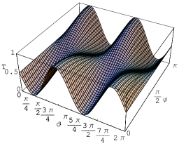
Figure 4: Electron transmittivity $T$ at $kx_{0}=n\pi$ and $\rho(E)J=10$ when the electron is injected in an arbitrary spin state $(\alpha\left|\uparrow\right\rangle+\beta\left|\downarrow\right\rangle)$ with the impurities prepared in the state $\cos{\vartheta}\left|\uparrow\downarrow\right\rangle+e^{i\varphi}\sin{\vartheta}\left|\downarrow\uparrow\right\rangle$.

In agreement with what was discussed in section 4, denoting by $T_{\Psi^{\pm}}$ the transmittivity for $\left|\Psi^{\pm}\right\rangle$, decoherence effects cause $T_{\Psi^{+}}<1$ (it gets smaller and smaller for increasing values of $\rho(E)J$) while $T_{\Psi^{-}}=1$ due to occurrence of perfect transparency. To explain why $T_{\Psi^{-}}$ and $T_{\Psi^{+}}$ are, respectively, maxima and minima of $T$, we observe that the set of states (29) is spanned by $\left|\Psi^{-}\right\rangle$ and $\left|\Psi^{+}\right\rangle$. Since these two states belong to orthogonal eigenspaces of the constant of motion $\mathbf{S}_{12}^{2}$ a linear combination of them cannot exhibit quantum interference effects and reduces to a statistical mixture. This ensures that the transmittivity for a generic state (29) will have intermediate values between $T_{\Psi^{+}}$ and $T_{\Psi^{-}}$.

The most remarkable result emerging from the above discussion is that, within the set of initial impurity spins states (29), maximally entangled states $\left|\Psi^{-}\right\rangle$ and $\left|\Psi^{+}\right\rangle$ have the relevant property of maximizing or minimizing electron transmission. We have chosen $\rho(E)J=10$ to better highlight this behaviour, but this happens for any value of $\rho(E)J$. This result suggests the appealing possibility to use the relative phase $\varphi$ as a control parameter to modulate the electron transmission in a 1D wire [12].

According to what was discussed in section 4, perfect transparency ensures that, once $\left|\Psi^{-}\right\rangle$ is set for obtaining high conductivity of the device, this impurity spins state will not be lost during transport of electrons through the wire. However, the same is not true for the low conductivity-state $\left|\Psi^{+}\right\rangle$ which is instead affected by spin-flip events and in general will be destroyed by electron scattering (see section 4). For the above entanglement controlled-modulation to be correctly performed, it is thus required that $\left|\Psi^{+}\right\rangle$ can be protected from spin-flip events. To achieve this, conservation of $\mathbf{S}_{12}^{2}$ can again be fruitfully used together with proper spin-filtering.

Assume thus that the electrons are injected in a fixed spin state, let us say $\left|\uparrow\right\rangle$. As discussed in section 4, in the regime $kx_{0}=n\pi$ conservation of $\mathbf{S}_{12}^{2}$ implies that $\left|\uparrow\right\rangle\left|\Psi^{+}\right\rangle$ is transmitted (or reflected) as a linear combination of $\left|\uparrow\right\rangle\left|\Psi^{+}\right\rangle$ and $\left|\downarrow\right\rangle\left|\uparrow\uparrow\right\rangle$. It follows that if the electrons are analyzed at the output of the wire in the same incoming spin state $\left|\uparrow\right\rangle$, the state $\left|\Psi^{+}\right\rangle$ of the impurity spins is protected from spin-flip [22].

Let us denote by $T_{+}$ the spin-polarized transmission amplitude that the electron is transmitted in the state $\left|\uparrow\right\rangle$. In figures 5(a) and (b) we have plotted $T$ and $T_{+}$, respectively, for an initial impurity spins state (29) with the electron injected in the state $\left|\uparrow\right\rangle$ and for $kx_{0}=n\pi$ and $\rho(E)J=2$. Note how $T_{\Psi^{+}}$ turns out to be lowered in figure 5(b) compared to 5(a). This is better visible in Fig. 5(c), where both $T$ and $T_{+}$, for $\varphi=0$, are plotted: in both cases maxima and minima occur for $\left|\Psi^{-}\right\rangle$ and $\left|\Psi^{+}\right\rangle$, respectively, but while maxima coincide, minima are lowered in the spin-filtered case. Spin-filtering thus allows the entanglement controlled-transmission task to work even more efficiently.

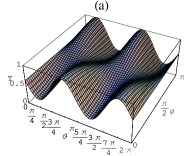
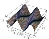
Figure 5: Electron transmittivity $T$ (a) and conditional electron transmittivity $T_{+}$ (b) at $kx_{0}=n\pi$ and $\rho(E)J=2$ when the electron is injected in the state $\left|\uparrow\right\rangle$ with the impurities prepared in the state $\cos{\vartheta}\left|\uparrow\downarrow\right\rangle+e^{i\varphi}\sin{\vartheta}\left|\downarrow\uparrow\right\rangle$. A comparison between $T$ (solid line) and $T_{+}$ (dashed line) for $\varphi=0$ is detailed in Fig. 5(c).

We have found that $T_{+}\simeq T$ for high values of $\rho(E)J$ as in figure 3 for $\rho(E)J=10$. Thus in these cases no spin-filtering is required to protect $\left|\Psi^{+}\right\rangle$.

Finally, we point out that the result showed in figure 4 opens the possibility of a new maximally entangled states detection scheme. Indeed, electron transmission can be regarded as a probe to detect maximally entangled singlet and triplet states of two localized spins within the family (29). In particular, it should be clear from the above discussion that use of spin-filtering makes the above setup a quantum non-demolition (QND) detection scheme both for $\left|\Psi^{-}\right\rangle$ and $\left|\Psi^{+}\right\rangle$. In particular, for the state $\left|\Psi^{-}\right\rangle$, such scheme works as a QND even without spin-filtering.

6 Transmission properties for aligned impurity spins states

Not all the sets of maximally entangled states exhibit the effects described in sections 3, 4 and 5. To show this, in this section, we consider a different family of impurity spins states

$$\left|\phi(\vartheta,\varphi)\right\rangle=\cos\vartheta\left|\uparrow\uparrow\right\rangle+e^{i\varphi}\sin\vartheta\left|\downarrow\downarrow\right\rangle$$ (32)

where again $\vartheta\in[0,2\pi]$ and $\varphi\in[0,\pi]$. Family (32) describes all the states in which the impurity spins are aligned.

The transmittivity $T$ for an electron incoming in the up spin state is shown in figures 6 (a), (b) and (c) for the cases $\vartheta=0$ (a), $\vartheta=\pi/2$ (b) and $\vartheta=\pi/4$ with arbitrary $\varphi$ (c). Note how the maximum of $T$ in the case of figure 6(c) has an intermediate value between the maximum of $T$ of figure 6(a) and the one of figure 6(b). Additionally, the results of figure 6(c) do not depend on the value of $\varphi$. The above behaviour can be easily understood once one realizes that, in the case of the initial spin state (32) the two impurities indeed behave as if they were prepared in the mixed state

$$\rho=\cos^{2}\vartheta\left|\uparrow\uparrow\right\rangle\langle{\uparrow\uparrow}|+\sin^{2}\vartheta\left|\downarrow\downarrow\right\rangle\langle{\downarrow\downarrow}|$$ (33)

The phase $\varphi$ thus plays no role for the present family of states and no interference effect occurs. The reason for this is that $\left|\uparrow\right\rangle\left|\uparrow\uparrow\right\rangle$ and $\left|\uparrow\right\rangle\left|\downarrow\downarrow\right\rangle$ are eigenstates of the constant of motion $S_{z}$ with different quantum numbers $m=3/2$ and $m=-1/2$, respectively. Therefore, unlike the set of states (29), no quantum interference effects are possible.

Additionally, note that while in the cases of figures 6 (b) and (c) a loss of electron coherence is exhibited similarly to the cases of figures 2(a), 2(b) and 3(a), a coherent behaviour completely analogous to a FP interferometer with partially silvered mirrors [8] is observed when the impurities are prepared in the state $\left|\uparrow\uparrow\right\rangle$ with the electron injected in the state $\left|\uparrow\right\rangle$, as illustrated in figure 6(a). Indeed, the spin state $\left|\uparrow\right\rangle\left|\uparrow\uparrow\right\rangle$ belongs to the non degenerate eigenspace $s=3/2$, $m=3/2$ where spin-flip does not occur and the impurities behave as if they were static (see subsection 2.1). However, we emphasize that at variance with perfect transparency induced by the impurities’ singlet state shown in figure 3(b), here $T=1$ for values of $kx_{0}$ depending on $\rho(E)J$ and only when the electron spin is initially aligned with the spins of the impurities.

The effect of transparency presented in figure 3(b) thus requires neither the knowledge of the coupling constant $J$ nor any constraint on the electron spin state to be observed.

Figure 6: Electron transmittivity $T$ as a function of $kx_{0}$ when the electron is injected in the state $\left|\uparrow\right\rangle$ with the impurities in the initial state $\left|\uparrow\uparrow\right\rangle$ (a), $\left|\downarrow\downarrow\right\rangle$ (b) and $(\left|\uparrow\uparrow\right\rangle+e^{i\varphi}\left|\downarrow\downarrow\right\rangle)/\sqrt{2}$ for arbitrary $\varphi$ (c). Dotted, dashed and solid lines stand for $\rho(E)J=1,2,10$, respectively.

7 Generation of entangled states

To observe the entanglement dependent electron transmittivity discussed in 3, 4 and 5 one must be able to prepare the maximally entangled states $\left|\Psi^{-}\right\rangle$ and $\left|\Psi^{+}\right\rangle$. In particular this is required to observe the entanglement controlled transmittivity illustrated in section 5. Although in our Hamiltonian model (1) there is no direct interaction between the two impurities, an indirect coupling via the electron spin takes place, as it is implicit in the non-kinetic part of $H$. In this section we thus show how electron-impurities scattering itself can be used to generate the desired entanglement between the impurity spins.

We first observe that it is enough to be able to generate only one of the two states $\left|\Psi^{-}\right\rangle$ and $\left|\Psi^{+}\right\rangle$ since they can be easily transformed into each other by simply introducing a relative phase shift by means of a local field. In the following, we therefore show how the triplet state $\left|\Psi^{+}\right\rangle$ can be generated by electron scattering. Generation of entangled states of two magnetic impurities via electron scattering in 1D systems has been recently investigated in [16, 17, 18, 19]. The basic idea is to inject an electron in the state $\left|\uparrow\right\rangle$ with the two impurities prepared in the state $\left|\downarrow\downarrow\right\rangle$. Due to conservation of $S_{z}$ the transmitted spin state is of the form

$$A\left|\uparrow\right\rangle\left|\downarrow\downarrow\right\rangle+B\left|\downarrow\right\rangle\left|\uparrow\downarrow\right\rangle+C\left|\downarrow\right\rangle\left|\downarrow\uparrow\right\rangle$$ (34)

It follows that if the transmitted electron is analyzed in the down spin state $\left|\downarrow\right\rangle$ the two impurities are projected in the entangled state $B\left|\uparrow\downarrow\right\rangle+C\left|\downarrow\uparrow\right\rangle$ (apart from a normalization factor) with probability $|B|^{2}+|C|^{2}$. For a fixed electron energy, this state is not maximally entangled for any strength of the electron-impurity coupling constant $J$ [17]. However in [17] the role played by the distance $x_{0}$ between the impurities was not taken into account. In the remaining of this section we will therefore consider an improved entanglement generation scheme [12] making use of the exact knowledge of the energy eigenstates developed above. In particular we will consider the regime $kx_{0}=n\pi$. In this case, in addition to $S_{z}$, also $\mathbf{S}_{12}^{2}$ becomes a constant of motion. It follows that the transmitted spin state will be of the form (see also section 4)

$$A^{\prime}\left|\uparrow\right\rangle\left|\downarrow\downarrow\right\rangle+B^{\prime}\left|\downarrow\right\rangle\left|\Psi^{+}\right\rangle$$ (35)

An output filter selecting only transmitted electrons in the state $\left|\downarrow\right\rangle$ can thus be used to project the impurities into the state $\left|\Psi^{+}\right\rangle$. Note that at variance with the analysis discussed in [17], this scheme ensures that a maximally entangled state is always generated whatever the value of $J$. Furthermore, we also know that this is the maximally entangled triplet state $\left|\Psi^{+}\right\rangle$. The spin-polarized probability $T_{-}$ for the electron to be transmitted in the state $\left|\downarrow\right\rangle$ - that is to project the impurities into $\left|\Psi^{+}\right\rangle$ - is plotted in figure 7 as a function of $\rho(E)J$.

Figure 7: Spin-polarized electron transmittivity $T_{-}$ at $kx_{0}=n\pi$ as a function of $\rho(E)J$ when the electron is injected in the state $\left|\uparrow\right\rangle$ with the impurities prepared in the state $\left|\downarrow\downarrow\right\rangle$.

A probability larger than 20% can be reached with $\rho(E)J\simeq 1$.

8 Conclusions

To discuss the possibility to observe the effects presented in this paper, in particular the entanglement controlled transport, let us assume an electron effective mass of $0.067\,m_{0}$ (as in GaAs quantum wires) and two quantum dots – each one of size 1 nm – as the impurities. Furthermore, the electron wavelength must be large enough for the contact electron-dot potential of our Hamiltonian model (1) to be valid. This constraint implies that the electron energy must not exceed 2 meV. In this case, requiring that $\rho(E)J\simeq 1$ (i.e., as shown in section 7, the optimal condition for generating entangled states of the impurities) we obtain $J\simeq$ 1 eVÅ, which appears to be a reasonable value of the electron-impurity coupling constant.

To prevent many-body effects, whose occurrence would make the single electron-approach adopted in this work not valid, electrons could be shot over an additional tunnel barrier before interacting with the impurities as proposed in [23, 24]. This would allow the injection of single electrons within a narrow energy range well separated from the Fermi energy. Alternatively, this task could be accomplished using a single-electron turnstile [25] as suggested e.g. in [24, 26].

Finally we would like to comment on the effects of decoherence on the interference phenomena described above. Some of the most interesting features of electron spin in semiconductor nanostructures are the long decoherence times, which is typically larger than 100 nanoseconds (but can exceed in some cases the microsecond) and the long coherence lengths, which can be longer than 100 micrometers. Our approach is therefore able to predict an observable effect. For instance for an electron energy of 2 meV, the resonance condition $kx_{0}=n\pi$ implies that $x_{0}$ must be in the order of 100 nm. A coherence length of this order of magnitude is common in a GaAs quantum wires at low temperatures (e.g. see [27]). Of course a stationary state approach to scattering like the one we have used must be complemented with a dissipative map for the evolution of the impurity spins when one is interested in the steady state which can be obtained by the repeated injection and detection of electrons in the wire.

In summary, in this paper we have considered a 1D wire with two embedded spin-1/2 magnetic impurities. This system can be regarded as the electron analogue of a Fabry Perot interferometer in which the two mirrors have internal spin degrees of freedom. Adopting an appropriate quantum waveguide theory approach, we have derived all the necessary transmission amplitudes at all orders in the electron-impurity coupling constant. This has allowed us to calculate the electron transmission properties for an arbitrary initial spin state of the overall system. The typical behaviour is a loss of electron coherence induced by spin-flip events due to scattering by the magnetic impurities. However, when the maximally entangled singlet state of the impurity spins is prepared, we have found that perfect transparency of the wire is obtained regardless of the electron spin state at wave vectors which do not depend on the electron-impurity coupling constant. In the same regime, we have found that electron transmittivity is maximized (minimized) by the singlet (triplet) entangled states of the impurity spins. This suggests a novel use of entanglement as a tool to modulate the conductivity of a 1D wire. Additionally, the electron transmission can be thought as a probe to detect maximally entangled singlet and triplet states of two localized spins. When spin-filtering is performed, this is a QND detection scheme for both these states, while it works as a QND detection scheme for the singlet state even without spin-filtering. These behaviours have been explained in terms of the Hamiltonian symmetries, showing that appropriate electron wave vectors allow for an effective conservation of the squared total spin of the two impurities. Finally, we have proposed a scheme to generate maximally entangled states via electron scattering regardless of the electron-impurity coupling constant.

9 Acknowledgments

The authors thank the support from CNR (Italy) and GRICES (Portugal). YO and VRV thank the support from Fundação para a Ciência e a Tecnologia (Portugal), namely through programs POCTI/POCI and projects POCI/MAT/55796/2004 QuantLog and POCTI-SFA-2-91, partially funded by FEDER (EU) as well as the SQIG-IT EMSAQC initiative.

Appendix A Set of perfectly “transparent” states

In this Appendix we demonstrate that the only spin state $\left|\chi\right\rangle$ allowing perfect transparency of figure 3(b) to occur is of the form $\left|\chi\right\rangle=\left(\alpha\left|\uparrow\right\rangle+\beta\left|\downarrow\right\rangle\right)\left|\Psi^{-}\right\rangle$. To this we impose that the incoming and transmitted state coincide for values of $kx_{0}$ which do not depend on $\rho(E)J$ . This yields the conditions

$$\langle s_{e2};s,m\left|\chi\right\rangle=\gamma_{s_{e2},s,m}(\chi)$$ (36)

Let us define the following matrix of transmission amplitudes in the subspace $s=1/2$

$$\textbf{t}=\left(\begin{array}[]{cc}t^{(0;1/2)}_{0}&t^{(1;1/2)}_{0}\\ t^{(0;1/2)}_{1}&t^{(1;1/2)}_{1}\end{array}\right)$$ (39)

Taking into account (27) and the selection rules for $s_{e2}$ and $s_{e2}^{\prime}$, conditions (36) reduce to an equation for $s=3/2$ and a homogenous linear system of two equations for $s=1/2$

$$\left(t^{(1;3/2)}_{1}-1\right)\langle 1;3/2,m\left|\chi\right\rangle = 0$$ (40)

$$\left(\textbf{t}-\textbf{I}\right)\times\left(\begin{array}[]{cc}\langle 0;1/2,m\left|\chi\right\rangle\\ \langle 1;1/2,m\left|\chi\right\rangle\end{array}\right) = 0$$ (43)

where I is the $2\times 2$ identity matrix.

Let us assume that $\left|\chi\right\rangle$ has a non vanishing projection on $s=3/2$. This means that $\langle 1;3/2,m\left|\chi\right\rangle\neq 0$ for at least one $m$ and condition (40) gives $t^{(1;3/2)}_{1}=1$ which implies $|t^{(1;3/2)}_{1}|^{2}=1$. $|t^{(1;3/2)}_{1}|^{2}$ is the transmittivity of a wire with two static impurities of potential $J/4$ (see subsection 2.1) which is completely analogous to a FP interferometer with partially reflecting mirrors. Since in this case a resonance condition (transmittivity 1) occurs at values of $kx_{0}$ depending on the mirror reflectivity [8], we conclude that $t^{(1;3/2)}_{1}=1$ cannot occur at values of $kx_{0}$ independent on $\rho(E)J$ as for the case of figure 3(b).

It follows that $\langle 1;3/2,m\left|\chi\right\rangle=0\,\,\forall\,\,m$ (remind that coefficients $t_{s_{e2}}^{(s_{e2}^{\prime};s)}$ are $m$-independent). This implies that the spin states allowing occurrence of perfect transparency must fully lie in the subspace $s=1/2$. Such states can be determined by requiring that linear system (43) has non trivial solutions, that is

$$\det{\left(\textbf{t-I}\right)}=0$$ (44)

which with the help of (2.2) and (2.2) is explicitly written as

$$\frac{3}{\delta}(e^{2ikx_{0}}-1)(\pi\rho(E)J)^{3}\left[3\pi\rho(E)J\,(e^{2ikx_{0}}-1)+32i\right]=0$$ (45)

with $\delta$ given by (25). Since the factor in square brackets cannot vanish for real $kx_{0}$ equation (45) is fulfilled for

$$kx_{0}=n\pi$$ (46)

with $n$ integer. Replacement of (46) in (43) yields the $\rho(E)J$-independent solution

$$\langle 0;1/2,m\left|\chi\right\rangle=\frac{\langle 1;1/2,m\left|\chi\right\rangle}{\sqrt{3}}$$ (47)

with arbitrary coefficients $\langle 0;1/2,m\left|\chi\right\rangle$ ($m=-1/2,1/2$). Rewriting these as $\langle 0;1/2,1/2\left|\chi\right\rangle=\alpha/2$ and $\langle 0;1/2,-1/2\left|\chi\right\rangle=\beta/2$, $\left|\chi\right\rangle$ turns out to be of the form

$$\left|\chi\right\rangle=\alpha\left(\frac{1}{2}\left|0;1/2,1/2\right\rangle+\frac{\sqrt{3}}{2}\left|1;1/2,1/2\right\rangle\right)+\beta\left(\frac{1}{2}\left|0;1/2,-1/2\right\rangle+\frac{\sqrt{3}}{2}\left|1;1/2,-1/2\right\rangle\right)$$

Using Clebsh-Gordan coefficients, spin states inside brackets turn out to be

$$\frac{1}{2}\left|0;1/2,1/2\right\rangle+\frac{\sqrt{3}}{2}\left|1;1/2,1/2\right\rangle = \left|\uparrow\right\rangle\left|\Psi^{-}\right\rangle$$ (49)

$$\frac{1}{2}\left|0;1/2,-1/2\right\rangle+\frac{\sqrt{3}}{2}\left|1;1/2,-1/2\right\rangle = \left|\downarrow\right\rangle\left|\Psi^{-}\right\rangle$$ (50)

Substitution of (49) and (50) into (A) proves that spin states exhibiting perfect transparency are of the form $\left|\chi\right\rangle=\left(\alpha\left|\uparrow\right\rangle+\beta\left|\downarrow\right\rangle\right)\left|\Psi^{-}\right\rangle$.

References

References

- [1] Mitin V, Kochelap V and Stroscio M 1999 Quantum Heterostructures: Microelectronics and Optoelectronics (Cambridge: Cambridge Univ. Press)
- [2] Davies J H 1998 The Physics of Low-Dimensional Semiconductors: an Introduction (Cambridge: Cambridge University Press)
- [3] Datta S 1995 Electronic Transport in Mesoscopic Systems (Cambridge : Cambridge Univ. Press)
- [4] Awschalom D D, Loss D and Samarth N 2002 Semiconductor Spintronics and Quantum Computation (Berlin : Springer)
- [5] Datta S and Das B 1990 Appl. Phys. Lett. 56 665
- [6] Loss D and Di Vincenzo D P 1998 Phys. Rev. A 57 120
- [7] Tans S J, Devoret M H, Dai H, Thess A, Smalley R E, Geerligs L J and Dekker C 1997 Nature 386 474
- [8] Rossi B Optics 1957 (London: Addison-Wesley)
- [9] Stern A, Aharonov Y and Imry Y 1990 Phys. Rev. A 41 3436
- [10] Imry Y 1997 Introduction to Mesoscopic Physics (New york: Oxford Univ. Press)
- [11] Schulman L S 1996 Phys. Lett. A 211 75
- [12] Ciccarello F, Palma G M, Zarcone M, Omar Y and Vieira V R 2006 New J. Phys. 8 214
- [13] Of course, we could also choose the scheme in which the electron is first coupled to impurity 1, while the scheme in which the two impurities are first coupled together is not convenient for the present problem.
- [14] de Menezes O L T and Helman J S 1985 Am. J. Phys. 53 1100
- [15] Mao J M, Huang Y and Zhou J M 1993 J. Appl. Phys. 73 1853
- [16] Yang D, Gu S-J and Li H 2005 ArXiv: quant-ph/0503131
- [17] Costa Jr. A T, Bose S and Omar Y 2006 Phys. Rev. Lett. 96 230501
- [18] Giorgi G. L. and De Pasquale F 2006 Phys. Rev. B 74 153308
- [19] Yuasa K and Nakazato H 2007 J. Phys. A 40 297
- [20] M. Weissbluth Atoms and Molecules 1978 (New York: Academic Press)
- [21] Joshi S K, Sahoo D and Jayannavar A M 2001 Phys. Rev. B 64 075320
- [22] We emphasize again that conservation of is crucial for this spin-flip protection scheme to work. Indeed, if the same spin-filtering procedure would leave the impurity spins in a linear combination of and , this state being in general different from .
- [23] Schomerus H, Noat Y, Dalibard J and Beenakker C W J 2002 Europhys. Lett. 57 651
- [24] Schomerus H and Robinson J P 2006 cond-mat/0604498
- [25] Kouwenhoven L P, Johnson A T, van der Vaart N C, Harmans C J P M and Foxon C T 1991 Phys. Rev. Lett. 67 1626
- [26] Jefferson J H, Ramsak A and Rejec 2006 Europhys. Lett. 74 764
- [27] Ferry D K and Goodnick S M 1997, Transport in Nanostructures (Cambridge : Cambridge Univ. Press)