Wigner formula of rotation matrices and quantum walks

Abstract

Quantization of a random-walk model is performed by giving a qudit (a multi-component wave function) to a walker at site and by introducing a quantum coin, which is a matrix representation of a unitary transformation. In quantum walks, the qudit of walker is mixed according to the quantum coin at each time step, when the walker hops to other sites. As special cases of the quantum walks driven by high-dimensional quantum coins generally studied by Brun, Carteret, and Ambainis, we study the models obtained by choosing rotation as the unitary transformation, whose matrix representations determine quantum coins. We show that Wigner’s $(2j+1)$-dimensional unitary representations of rotations with half-integers $j$’s are useful to analyze the probability laws of quantum walks. For any value of half-integer $j$, convergence of all moments of walker’s pseudovelocity in the long-time limit is proved. It is generally shown for the present models that, if $(2j+1)$ is even, the probability measure of limit distribution is given by a superposition of $(2j+1)/2$ terms of scaled Konno’s density functions, and if $(2j+1)$ is odd, it is a superposition of $j$ terms of scaled Konno’s density functions and a Dirac’s delta function at the origin. For the two-, three-, and four-component models, the probability densities of limit distributions are explicitly calculated and their dependence on the parameters of quantum coins and on the initial qudit of walker is completely determined. Comparison with computer simulation results is also shown.

I INTRODUCTION

No one doubts the importance of random-walk models in physics, mathematics and computer sciences. In particular, when we explain basic concepts of statistical physics Rei65 , stochastic processes in physics and chemistry vKam92 , and stochastic algorithms MR95 , introduction of random-walk models is very useful and effective. It is interesting to see that systematic study of quantization of random walks is not old ADZ93 ; Mey96 ; NV00 ; ABNVW01 . As expected, the study of quantum walks is fruitful and its results have been applied to solve the transport problems in solid-state physics of strongly correlated electron systems Oka05 , to derive non-Gaussian-type central limit theorems in probability theory Kon02 ; Kon05a ; GJS04 , and to invent new algorithms in the quantum information theory Gro97 ; Amb04 . The research field of quantum walks is growing widely Kem03 ; TFMK03 ; Amb03 ; MBSS02 ; BCA03 ; Ken06 and mathematical understanding of the new models is becoming deeper Kon05b ; GJS05 ; Kon06 ; Oba06 ; Kon07 in recent years.

It should be noted here that, from the view-point of standard quantum mechanics, “to quantize random walks” is a contradictory concept, since in quantum mechanics, time-evolution of a state vector $|\Psi(t)\rangle$, or a wave function $\Psi(x,t)$, is given by a deterministic unitary transformation associated with the Hamiltonian and probability concept appears in the theory only when we perform observation of physical quantities, i.e., when we calculate the probability density $p(x,t)=|\Psi(x,t)|^{2}$ at a given time. On the other hand, random walk is a typical example of stochastic processes, in which we toss a coin to select a walk at each time step. In an earlier paper KFK05 , it was shown that the one-dimensional standard random walk can be realized by a random-turn model Kon03 , in which a coin is represented by a $2\times 2$ stochastic matrix and that, if we replace the matrix by a $2\times 2$ unitary matrix, a one-dimensional quantum-walk model is obtained. This argument is not only heuristic but also generic, since it implies that quantization of random-walk models can be done by introducing appropriate unitary matrices such that they play the roles of “quantum coins”. The obtained time-evolution of quantum walk is described by multi-component version of quantum-mechanical equation of motion. For the standard quantum-walk model on one-dimensional lattice ${\bf Z}=\{\cdots,-2,-1,0,1,2,\cdots\}$ with the nearest-neighbor hopping, the equation is identified with the Weyl equation for two-component wave functions KFK05 . It should be remarked that such multi-component equations have been usually used in relativistic quantum mechanics BES06 .

It should be noted that in order to discuss the relationship between classical and quantum walks Brun et al. showed a method to construct discrete quantum-walk models for multi-component wave functions driven by high-dimensional quantum coins that are greater than $2\times 2$ matrices BCA03 . There they considered a $2^{M}$-dimensional space with $M=2,3,\cdots$, whose basis is given by tensor products of $M$ binary-vectors. A quantum coin, which is first defined as an abstract unitary transformation $\hat{U}$, has a $2^{M}\times 2^{M}$ matrix representation in the space BCA03 . Their method is very general and useful as well as the tensor-product method is in the group representation theory Geo99 . See also Refs. MBSS02 ; BCA03b ; VBBB05 for tensor-product models.

In the present paper, we adopt the rotation operator $\hat{R}$ specified by the Euler angles $\alpha,\beta,\gamma$ (see Eq.(3) in Sec.II) as the unitary transformation $\hat{U}$ and introduce a family of quantum-walk models on one-dimensional lattice ${\bf Z}$. The two-dimensional representations of $\hat{R}$ can be identified with $2\times 2$ quantum-coin matrices used in the standard quantum walks with qubits. In the wave-number space ($k$-space) the shift matrix $S(k)$ is generally given by a matrix representation of $\hat{R}$, if we set the parameters $\alpha=-2k,\beta=\gamma=0$ (see Sec.III). Our choice $\hat{U}=\hat{R}$ is thus very suitable to study one-dimensional quantum walk problems.

Instead of using the tensor-product representations following Brun et al., we will use in this paper the $(2j+1)$-dimensional unitary representations $R^{(j)}(\alpha,\beta,\gamma)$ of the rotation operator $\hat{R}$ with half-integers $j$’s as quantum coins, which are called the rotation matrices Mes75 . The reason is the following. The $2^{M}$-dimensional representations with $M\geq 2$ constructed by tensor products are reducible; By changing basis through appropriate orthogonal transformations, tensor-product matrices are block-diagonalized. Wigner’s theory showed that each block with size $2j+1\,(j=0,1/2,1,3/2,\cdots)$ is given by a rotation matrix $R^{(j)}(\alpha,\beta,\gamma)$ Wig59 . In other words, we will use the irreducible representations of $\hat{R}$. In Sec.IV, reducibility of the tensor-product models of quantum walks to the present models will be generally shown and demonstrated using examples.

In our model with $j$ and three parameters $(\alpha,\beta,\gamma)$, a quantum walker is assumed to be at the origin at time $t=0$ with a $(2j+1)$-component qudit

$$\phi_{0}^{(j)}=\left(\begin{array}[]{c}q_{j}\cr q_{j-1}\cr\cdots\cr q_{-j+1}\cr q_{-j}\end{array}\right)\quad\mbox{with}\quad\sum_{m=-j}^{j}|q_{m}|^{2}=1,$$ (1)

where $q_{m}\in{\bf C}$(complex numbers), $m=-j,-j+1,\cdots,j$. At each time step $t=1,2,3,\cdots$, the components of qudit are mixed according to a quantum coin $R^{(j)}(\alpha,\beta,\gamma)$ and the walker hops to $(2j+1)$ sites on ${\bf Z}$, as illustrated by Fig.1 for $j=1/2,1,3/2$ and 2 (see Eq.(18) in Sec.III). When $j=1/2$, $R^{(1/2)}(\alpha,\beta,\gamma)$ can be identified with an element of SU(2) appropriately parameterized by the three variables (the Cayley-Klein parameters) and the model is reduced to the standard two-component model KFK05 . It should be noted here that, when $j$ is an integer (i.e. $(2j+1)$ is odd), the walker can stay at the same position in a step.

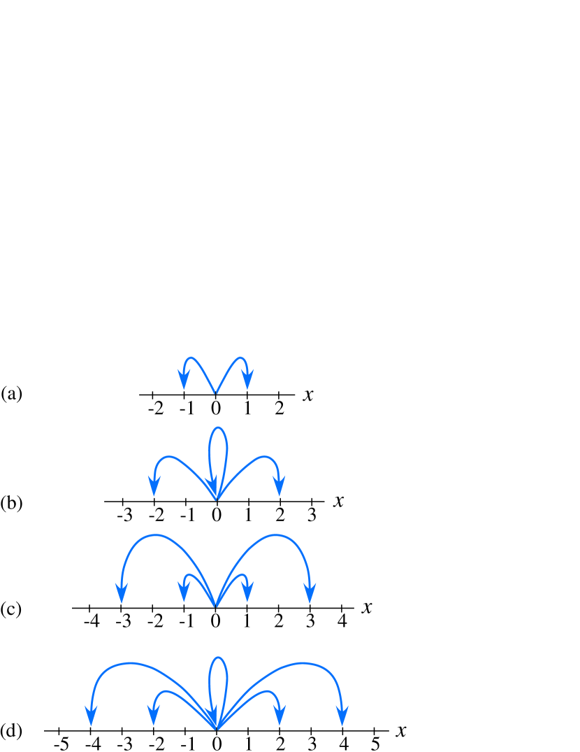
Figure 1: (Color online) Elementary hopping of quantum walker in the models with (a) $j=1/2$ (two-component model), (b) $j=1$ (three-component model), (c) $j=3/2$ (four-component model), and (d) $j=2$ (five-component model). When $(2j+1)$ is odd, the walker can stay at the same position in a step, as shown by cyclic arrows at the origin in the cases (b) and (d).

Using the method of GJS04 , we will prove that any moments of pseudovelocity of walker, which is defined by $X_{t}/t$ (the position at time $t$, $X_{t}$, divided by $t$), converges in the long-time limit $t\to\infty$, and show that the probability measure of limit distribution is generally described by a superposition of appropriately scaled forms of a function

$$\mu(x;a)=\frac{\sqrt{1-a^{2}}}{\pi(1-x^{2})\sqrt{a^{2}-x^{2}}}{\bf 1}_{\{|x|<|a|\}},$$ (2)

where ${\bf 1}_{\{\omega\}}$ denotes the indicator function of a condition $\omega$; ${\bf 1}_{\{\omega\}}=1$ if $\omega$ is satisfied and ${\bf 1}_{\{\omega\}}=0$ otherwise, and $a$ is a real parameter. It is the density function first introduced by Konno to describe the limit distributions of the standard two-component quantum walks in his weak limit-theorem Kon02 ; Kon05a . (As shown in Fig.2(a) in Sec.VI, $\mu(x;a)$ is inversed bell-shaped on a finite support $x\in(-a,a)$ in big contrast with the Gaussian distribution, which describes the diffusion scaling limit of the classical random walks.) More precisely speaking, when $(2j+1)$ is even, the probability density function of limit distribution consists of $(2j+1)/2$ terms of Konno’s density functions (2), and when $(2j+1)$ is odd, it does of $j$ terms of Konno’s and a point mass at the origin, which corresponds to the positive probability to retain the position of walker in a step (see Eq.(94)).

The weight functions ${\cal M}^{(j,m)}$ of these Konno’s density functions (and the weight $\Delta^{(j)}$ of Dirac’s delta function at the origin, when $(2j+1)$ is odd) in the superposition depend on the parameters of quantum coin and the $(2j+1)$ components of initial qudit (1) of quantum walker. We have found that the representation theory of groups Geo99 is useful to calculate the weight functions. Especially the Wigner formula for rotation matrices Mes75 ; Wig59 is critical. In this paper we give the explicit forms of weight functions for $j=1/2,1$ and 3/2 (two-, three- and four-component models, respectively) and these results imply that the weight functions ${\cal M}^{(j,m)}$ are generally given by polynomials. Through these polynomials, the initial-qudit dependence of the limit distribution of pseudovelocity is completely determined.

This paper is organized as follows. In Sec.II, Wigner formula of $(2j+1)$-dimensional irreducible representation of the rotation group SO(3) is summarized. The family of quantum-walk models associated with the rotation matrices is defined for quantum walkers with $(2j+1)$-component qudit in Sec.III. In Sec.IV we also introduce the tensor-product models of one-dimensional quantum walks associated with the rotation operator $\hat{R}$ following the general theory of Brun et al. BCA03 . There we show the reducibility of the tensor-product models to our models. Sec.V is devoted to proving the generalized weak limit-theorem (convergence of all moments) for pseudovelocities of quantum walks. There the polynomials, which give the weights of Konno’s density functions and the point mass in the limit distributions, are listed for $j=1/2,1$ and 3/2, explicitly. Comparison with computer simulation with the present analytic results is given in Sec.VI. In this last section, we also discuss relations between our results and other multi-component models BCA03 ; BCA03b ; IK05 ; IKS05 ; VBBB05 ; IKK04 and possible future problems.

II WIGNER FORMULA OF $(2j+1)$-DIMENSIONAL REPRESENTATIONS OF ROTATION GROUP

Any rotation in the three-dimensional real space ${\bf R}^{3}$ is uniquely specified by three rotation angles $\alpha,\beta,\gamma$ called the Euler angles. In the quantum mechanics, the rotation with the Euler angles $\alpha,\beta,\gamma$ is given by an operator of the form (see, for instance, Mes75 )

$$\hat{R}(\alpha,\beta,\gamma)=e^{-{\rm i}\alpha\hat{J}_{3}}e^{-{\rm i}\beta\hat{J}_{2}}e^{-{\rm i}\gamma\hat{J}_{3}},$$ (3)

where $\hat{\bf J}=(\hat{J}_{1},\hat{J}_{2},\hat{J}_{3})$ is the vector operator of angular momentum, whose elements satisfy the su(2) Lie algebra,

$$[\hat{J}_{k},\hat{J}_{\ell}]={\rm i}\sum_{m=1}^{3}\varepsilon_{k\ell m}\hat{J}_{m},\quad k,\ell=1,2,3,$$ (4)

with the completely antisymmetrical tensor with three indices $\varepsilon_{k\ell m}$ Geo99 . Let the ket-vector $|j,m\rangle,j=0,1/2,1,3/2,\cdots,m=-j,-j+1,\cdots,j$, denote the normalized eigenstates of $\hat{\bf J}^{2}=\sum_{k=1}^{3}\hat{J}_{k}^{2}$ and $\hat{J}_{3}$ such that $\hat{\bf J}^{2}|j,m\rangle=j(j+1)|j,m\rangle$, and $\hat{J}_{3}|j,m\rangle=m|j,m\rangle$. (We set $\hbar=1$ in this paper.) Then, for each fixed value of half-integer $j$, a $(2j+1)\times(2j+1)$ unitary matrix $R^{(j)}(\alpha,\beta,\gamma)=(R^{(j)}_{mm^{\prime}}(\alpha,\beta,\gamma))$ is defined with its elements

$$R^{(j)}_{mm^{\prime}}(\alpha,\beta,\gamma)=\langle j,m|\hat{R}(\alpha,\beta,\gamma)|j,m^{\prime}\rangle,$$ (5)

$m,m^{\prime}=-j,-j+1,\cdots,j$. We can show that

$$R^{(j)}_{mm^{\prime}}(\alpha,\beta,\gamma)=e^{-{\rm i}\alpha m}r^{(j)}_{mm^{\prime}}(\beta)e^{-{\rm i}\gamma m^{\prime}}$$ (6)

with

$$r^{(j)}_{mm^{\prime}}(\beta) = \sum_{\ell}\Gamma(j,m,m^{\prime},\ell)$$ (7)

$$\times \left(\cos\frac{\beta}{2}\right)^{2j+m-m^{\prime}-2\ell}\left(\sin\frac{\beta}{2}\right)^{2\ell+m^{\prime}-m},$$

where

$$\Gamma(j,m,m^{\prime},\ell)$$

$$=(-1)^{\ell}\frac{\sqrt{(j+m)!(j-m)!(j+m^{\prime})!(j-m^{\prime})!}}{(j-m^{\prime}-\ell)!(j+m-\ell)!\ell!(\ell+m^{\prime}-m)!}.\quad$$ (8)

In (7) the summation $\sum_{\ell}$ extends over all integers of $\ell$ for which the arguments of the factorials are positive or null ($0!=1$). The matrix (6) gives a $(2j+1)$-dimensional irreducible representation of the rotation group SO(3) and is called the rotation matrix. Eq.(7) is known as the Wigner formula Mes75 ; Wig59 . In the present paper, when we write matrices and vectors whose elements are labeled by $m,m^{\prime}$, we will assume that the indices $m$ and $m^{\prime}$ run from $j$ to $-j$ in steps of $-1$. In Appendix A, we give explicit expressions of matrices $r^{(j)}(\beta)=(r^{(j)}_{mm^{\prime}}(\beta))$ for $j=1/2,1$ and 3/2.

III QUANTUM-WALK MODELS WITH $(2j+1)$-COMPONENT QUDITS

Here we propose a new family of models of quantum walks on the one-dimensional lattice ${\bf Z}$, in which each walker has a $(2j+1)$-component qudit (1). In the previous paper KFK05 , we reported the weak limit-theorem for the two-component model. That model is generated by a quantum coin represented by a matrix in SU(2)

$$A=\left(\begin{array}[]{cc}ue^{{\rm i}\theta}&\sqrt{1-u}e^{{\rm i}\phi}\cr-\sqrt{1-u^{2}}e^{-{\rm i}\phi}&ue^{-{\rm i}\theta}\end{array}\right),$$ (11)

$$\qquad u\in[-1,1],\,\theta,\phi\in[-\pi,\pi)$$ (12)

and a spatial shift-operator on ${\bf Z}$, which is represented by a matrix

$$S(k)=\left(\begin{array}[]{cc}e^{{\rm i}k}&0\cr 0&e^{-{\rm i}k}\end{array}\right),\quad k\in[-\pi,\pi)$$ (13)

in the $k$-space. If we compare these matrices with (6) with $j=1/2$ and (111) in Appendix A, we find that they are the special cases of $R^{(1/2)}(\alpha,\beta,\gamma)$;

$$A = R^{(1/2)}(\pi-\theta-\phi,2{\rm arccos}(u),-\pi-\theta+\phi),$$

$$S(k) = R^{(1/2)}(-2k,0,0).$$ (14)

From the view point of the group theory, we can give the following remark. In KFK05 we used the fact that SU(2)$\simeq{\bf S}^{3}$ ($\equiv$ the three dimensional unit sphere in ${\bf R}^{4}$) and the quantum coin $A$ was parameterized by three real numbers, $u,\theta,\phi$ (the Cayley-Klein parameters), corresponding the dimensionality 3 of the group space. On the other hand, we are now regarding the quantum coin $A$ as a two-dimensional representation of the rotation group SO(3), and thus the three parameters are identified with the Euler angles for rotations in the three-dimensional real-space ${\bf R}^{3}$.

This observation had led us to adopt the $(2j+1)$-dimensional representation of the rotation group, $R^{(j)}(\alpha,\beta,\gamma)$, as a quantum coin to mix $(2j+1)$ components in qudit (1). The spatial shift-matrix is given by $S^{(j)}(k)=R^{(j)}(-2k,0,0)={\rm diag}(e^{2{\rm i}jk},e^{2{\rm i}(j-1)k},\cdots,e^{-2{\rm i}jk})$.

We assume at the initial time $t=0$ that the walker is located at the origin. Then, in the $k$-space, the $(2j+1)$-component wave function of the walker at time $t$ is given by

$$\hat{\Psi}^{(j)}(k,t)=\Big{(}V^{(j)}(k)\Big{)}^{t}\phi_{0}^{(j)},\quad t=0,1,2,\cdots,$$ (15)

where

$$V^{(j)}(k) = V^{(j)}(k;\alpha,\beta,\gamma)$$ (16)

$$\equiv S^{(j)}(k)R^{(j)}(\alpha,\beta,\gamma)$$

$$= R^{(j)}(\alpha-2k,\beta,\gamma).$$

The time evolution in the real space ${\bf Z}$ is then obtained by performing the Fourier transformation,

$$\Psi^{(j)}(x,t) = \int_{-\pi}^{\pi}\frac{dk}{2\pi}\hat{\Psi}^{(j)}(k,t)e^{{\rm i}kx},$$

$$\hat{\Psi}^{(j)}(k,t) = \sum_{x\in{\bf Z}}\Psi^{(j)}(x,t)e^{-{\rm i}kx},$$ (17)

as

$$\Psi^{(j)}_{m}(x,t+1)=\sum_{m^{\prime}=-j}^{j}R^{(j)}_{mm^{\prime}}\Psi^{(j)}_{m^{\prime}}(x+2m,t),\,t=0,1,2,\cdots,$$ (18)

where $\Psi^{(j)}_{m}(x,t)$ denotes the $m$-th component of the $(2j+1)$-component wave function $\Psi^{(j)}(x,t)$.

Now the stochastic process of $(2j+1)$-component quantum walk is defined on ${\bf Z}$ as follows. Let $X^{(j)}_{t}$ be the position of the walker at time $t$. The probability that we find the walker at site $x\in{\bf Z}$ at time $t$ is given by

$${\rm Prob}(X^{(j)}_{t}=x)=P(x,t)=[\Psi^{(j)}(x,t)]^{\dagger}\Psi^{(j)}(x,t),$$ (19)

where $[\Psi^{(j)}(x,t)]^{\dagger}$ is the hermitian conjugate of $\Psi^{(j)}(x,t)$. As shown in KFK05 , the $r$-th moment of $X^{(j)}_{t}$ is given by

$$\langle(X^{(j)}_{t})^{r}\rangle \equiv \sum_{x\in{\bf Z}}x^{r}P(x,t)$$ (20)

$$= \int_{-\pi}^{\pi}\frac{dk}{2\pi}[\hat{\Psi}^{(j)}(k,t)]^{\dagger}\left({\rm i}\frac{d}{dk}\right)^{r}\hat{\Psi}^{(j)}(k,t),$$

$$\qquad r=0,1,2,\cdots.$$

IV TENSOR PRODUCT MODELS ASSOCIATED WITH ROTATION OPERATOR AND THEIR REDUCIBILITY

IV.1 Tensor product models

In this section we use the notation $|1\rangle=|1/2,1/2\rangle$, $|-1\rangle=|1/2,-1/2\rangle$ for the binary states with $j=1/2$. Let $M\in\{2,3,4,\cdots\}$. For an $M$-component variable ${\bf m}=(m_{1},m_{2},\cdots,m_{M})$ with $m_{n}\in\{-1,1\},1\leq n\leq M$, we will write $|{\bf m}|=\sum_{n=1}^{M}m_{n}$.

Following Brun et al. BCA03 we consider the $2^{M}$-dimensional space spanned by the bases $\{|{\bf m}\rangle\}_{{\bf m}\in\{-1,1\}^{M}}$, which are defined as tensor products

$$|{\bf m}\rangle=\prod_{n=1}^{M}|m_{n}\rangle.$$ (21)

Note that they are orthonormal; $\langle{\bf m}|{\bf m}^{\prime}\rangle=\delta_{{\bf m},{\bf m}^{\prime}}\equiv\prod_{n=1}^{M}\delta_{m_{n}m_{n}^{\prime}}$. Let

$${\rm R}^{[M]}_{{\bf m},{\bf m}^{\prime}}(\alpha,\beta,\gamma)=\langle{\bf m}|\hat{R}(\alpha,\beta,\gamma)|{\bf m}^{\prime}\rangle,$$

and define a $2^{M}\times 2^{M}$ matrix ${\rm R}^{[M]}(\alpha,\beta,\gamma)=({\rm R}^{[M]}_{{\bf m},{\bf m}^{\prime}}(\alpha,\beta,\gamma))_{{\bf m},{\bf m}^{\prime}\in\{-1,1\}^{M}}$. By definition of tensor products Geo99 ,

$${\rm R}^{[M]}_{{\bf m},{\bf m}^{\prime}}(\alpha,\beta,\gamma) = \prod_{n=1}^{M}R^{(1/2)}_{m_{n}/2,m_{n}^{\prime}/2}(\alpha,\beta,\gamma)$$

$$= e^{-{\rm i}\alpha|{\bf m}|/2-{\rm i}\gamma|{\bf m}^{\prime}|/2}\prod_{n=1}^{M}r^{(1/2)}_{m_{n}/2,m_{n}^{\prime}/2}(\beta),$$

where $r^{(1/2)}(\beta)=(r^{(1/2)}_{m/2,m^{\prime}/2})_{m,m^{\prime}\in\{-1,1\}}$ is given by (111) in Appendix A. This gives a $2^{M}$-dimensional tensor-product representation of the rotation group. Define the shift matrix in the $k$-space by ${\rm S}^{[M]}_{{\bf m},{\bf m}^{\prime}}(k)={\rm R}^{[M]}_{{\bf m},{\bf m}^{\prime}}(-2k,0,0)=e^{{\rm i}k|{\bf m}|}\delta_{{\bf m}{\bf m}^{\prime}},$ and set

$${\rm V}^{[M]}(k) = {\rm S}^{[M]}(k){\rm R}^{[M]}(\alpha,\beta,\gamma)$$ (22)

$$= {\rm R}^{[M]}(\alpha-2k,\beta,\gamma).$$

Following the general theory of Brun et al. BCA03 , the wave function in the $k$-space at time $t$ of the one-dimensional quantum walk associated with the above tensor-product representation of SO(3) will be given by

$$\hat{\Phi}^{[M]}(k,t)=\Big{(}{\rm V}^{[M]}(k)\Big{)}^{t}\varphi_{0}^{[M]},\quad t=0,1,2,\cdots,$$ (23)

where the initial state is given by the $2M$-component qudit

$$\varphi_{0}^{[M]}=\bigotimes_{n=1}^{M}\left(\begin{array}[]{c}Q_{n}^{+}\cr Q_{n}^{-}\end{array}\right),\quad Q_{n}^{+},Q_{n}^{-}\in{\bf C}$$ (24)

with the normalization $\sum_{n=1}^{M}(|Q_{n}^{+}|^{2}+|Q_{n}^{-}|^{2})=1$. The real-space wave function is then given by its Fourier transformation

$$\Phi^{[M]}(x,t)=\int_{-\pi}^{\pi}\frac{dk}{2\pi}\hat{\Phi}^{[M]}(k,t)e^{{\rm i}kx}.$$ (25)

Let $Y_{t}^{[M]},t=0,1,2,\cdots,$ be the position of the walker at time $t$ of this tensor-product model. The probability distribution function is defined by

$$P^{[M]}(x,t)\equiv{\rm Prob}(Y^{[M]}_{t}=x)=[\Phi^{[M]}(x,t)]^{\dagger}\Phi^{[M]}(x,t).$$ (26)

The initial position of this quantum walk is the origin, $Y_{0}^{[M]}=0$, and the walker has the initial qudit (24).

IV.2 Reduction of quantum-walk models

Irreducible representations of the rotation group are given in the spaces spanned by $|j,m\rangle$, $j=0,1/2,1,3/2,\cdots$, $m=-j,-j+1,\cdots,j-1,j$ Wig59 ; Geo99 . The two kinds of bases $\{|{\bf m}\rangle\}$ and $\{|j,m\rangle^{\ell_{j}}\}$ are related through

$$|{\bf m}\rangle=\sum_{j}\sum_{\ell_{j}=1}^{d_{j}}\sum_{m_{j}}|j,m_{j}\rangle^{\ell_{j}}{\rm K}_{(j,m_{j})^{\ell_{j}},{\bf m}}$$ (27)

with

$${\rm K}^{[M]}_{(j,m_{j})^{\ell_{j}},{\bf m}}=^{\ell_{j}}\!\langle j,m_{j}|{\bf m}\rangle,$$ (28)

where $d_{j}$ is the multiplicity of the $(2j+1)$-dimensional irreducible representations included in the $2^{M}$-dimensional tensor-product representation and for each $j$ an index $\ell_{j}$ runs from 1 to $d_{j}$. Remark that $\sum_{j}d_{j}(2j+1)=2^{M}$. Define the $2^{M}$-dimensional matrix ${\rm K}^{[M]}=({\rm K}^{[M]}_{(j,m_{j})^{\ell_{j}},{\bf m}})$, which is an orthogonal matrix; $({\rm K}^{[M]})^{-1}=^{t}\!{\rm K}^{[M]}$.

Then we see

$${\rm K}^{[M]}{\rm R}^{[M]}(\alpha-2k,\beta,\gamma)({\rm K}^{[M]})^{-1}$$ (29)

$$= \bigoplus_{j,\ell_{j}}R^{(j,\ell_{j})}(\alpha-2k,\beta,\gamma)$$

$$= \bigoplus_{j}\Big{\{}R^{(j,1)}(\alpha-2k,\beta,\gamma)\oplus\cdots$$

$$\qquad\qquad\oplus R^{(j,d_{j})}(\alpha-2k,\beta,\gamma)\Big{\}},$$

where $R^{(j,\ell_{j})},\ell=1,2,\cdots,d_{j}$, are $d_{j}$ copies of the $(2j+1)$-dimensional irreducible representation of rotation group explained in Sec.II. That is, ${\rm R}^{[M]}(\alpha-2k,\beta,\gamma)$ can be block-diagonalized into a direct sum of rotation matrices. Note that direct sums in (29) and equations below are taken only over $j$’s such that ${\rm K}^{[M]}_{(j,m_{j})^{\ell_{j}},{\bf m}}\not=0$. (See the examples in the following subsection.) For (22) it implies that

$$({\rm V}^{[M]}(k))^{t}=({\rm K}^{[M]})^{-1}\bigoplus_{j,\ell_{j}}(V^{(j,\ell_{j})}(k))^{t}{\rm K}^{[M]},$$ (30)

where $V^{(j,\ell_{j})}(k)$ is the $\ell_{j}$-th copy of (16).

Let

$${\rm K}^{[M]}\varphi_{0}^{[M]}=\bigoplus_{j,\ell_{j}}\varphi_{0}^{(j,\ell_{j})},$$ (31)

and define

$$p^{(j,\ell_{j})}=[\varphi_{0}^{(j,\ell_{j})}]^{\dagger}\varphi_{0}^{(j,\ell_{j})}.$$ (32)

Then it is easy to prove that the probability distribution function (26) is decomposed as

$$P^{[M]}(x,t)=\sum_{j}\sum_{\ell_{j}=1}^{d_{j}}p^{(j,\ell_{j})}P^{(j,\ell_{j})}(x,t),$$ (33)

where $P^{(j,\ell_{j})}(x,t)$ is the probability distribution function of our quantum-walk model introduced in Sec.III, whose initial $(2j+1)$-component qudit is given by

$$\phi_{0}^{(j,\ell_{j})}=\frac{1}{\sqrt{p^{(j,\ell_{j})}}}\varphi_{0}^{(j,\ell_{j})}.$$ (34)

By this formula, the probability laws of quantum walks of the tensor-product models are completely determined by those of the models studied in the present paper.

IV.3 Examples

$M=2$ case  We set the $2^{2}=4$ states $\{|(m_{1},m_{2})\rangle\}_{(m_{1},m_{2})\in\{-1,1\}^{2}}$ in the order $|(1,1)\rangle$, $|(1,-1)\rangle$, $|(-1,1)\rangle$, $|(-1,-1)\rangle$. Then we have ${\rm R}^{[2]}_{{\bf m},{\bf m}^{\prime}}(\alpha,\beta,\gamma)=e^{-{\rm i}\alpha(m_{1}+m_{2})-{\rm i}\gamma(m_{1}^{\prime}+m_{2}^{\prime})}{\rm r}^{[2]}_{{\bf m},{\bf m}^{\prime}}$ with

$${\rm r}^{[2]}=\Big{(}{\rm r}^{[2]}_{{\bf m},{\bf m}^{\prime}}\Big{)}=\left(\begin{array}[]{cccc}c^{2}&-cs&-cs&s^{2}\cr cs&c^{2}&-s^{2}&-cs\cr cs&-s^{2}&c^{2}&-cs\cr s^{2}&cs&cs&c^{2}\end{array}\right).$$ (35)

The shift matrix is given in the $k$-space by

$${\rm S}^{[2]}(k)={\rm R}^{[2]}(-2k,0,0)=\left(\begin{array}[]{cccc}e^{2{\rm i}k}&0&0&0\cr 0&1&0&0\cr 0&0&1&0\cr 0&0&0&e^{-2{\rm i}k}\end{array}\right).$$ (36)

From the above four states, $\{|j,m\rangle:j=1,0\}$ are obtained by the highest weight construction (see, for example, Geo99 ) and we find the transformation matrix ${\rm K}^{[2]}$ as

$${\rm K}^{[2]}=\Big{(}\langle j,m|(m_{1},m_{2})\rangle\Big{)}=\left(\begin{array}[]{cccc}1&0&0&0\cr 0&\sqrt{1/2}&\sqrt{1/2}&0\cr 0&0&0&1\cr 0&\sqrt{1/2}&-\sqrt{1/2}&0\end{array}\right).$$ (37)

It is easy to confirm that

$${\rm K}^{[2]}{\rm r}^{[2]}(\beta)({\rm K}^{[2]})^{-1} = \left(\begin{array}[]{cccc}c^{2}&-\sqrt{2}cs&s^{2}&0\cr\sqrt{2}cs&2c^{2}-1&-\sqrt{2}cs&0\cr s^{2}&\sqrt{2}cs&c^{2}&0\cr 0&0&0&1\end{array}\right)$$ (42)

$$= r^{(1)}(\beta)\oplus 1,$$ (43)

where $r^{(1)}(\beta)$ is given by (111) in Appendix A. This implies ${\rm K}^{[2]}{\rm V}^{[2]}(k)({\rm K}^{[2]})^{-1}=V^{(1)}(k)\oplus 1.$ This decomposition will be symbolically denoted as

$$2\otimes 2=3\oplus 1.$$ (44)

$M=3$ case  We set the $2^{3}=8$ states $\{|(m_{1},m_{2},m_{3})\rangle\}_{(m_{1},m_{2},m_{3})\in\{-1,1\}^{3}}$ in the order $|(1,1,1)\rangle$, $|(1,1,-1)\rangle$, $|(1,-1,1)\rangle$, $|(1,-1,-1)\rangle$, $|(-1,1,1)\rangle$, $|(-1,1,-1)\rangle$, $|(-1,-1,1)\rangle$, $|(-1,-1,-1)\rangle$. Then we have ${\rm R}^{[3]}_{{\bf m},{\bf m}^{\prime}}(\alpha,\beta.\gamma)=e^{-{\rm i}\alpha(m_{1}+m_{2}+m_{3})-{\rm i}\gamma(m_{1}^{\prime}+m_{2}^{\prime}+m_{3}^{\prime})}{\rm r}^{[3]}_{{\bf m},{\bf m}^{\prime}}$ with

$${\rm r}^{[3]}=\Big{(}{\rm r}^{[3]}_{{\bf m},{\bf m}^{\prime}}\Big{)}=\left(\begin{array}[]{cccccccc}c^{3}&-c^{2}s&-c^{2}s&cs^{2}&-c^{2}s&cs^{2}&cs^{2}&-s^{3}\cr c^{2}s&c^{3}&-cs^{2}&-c^{2}s&-cs^{2}&-c^{2}s&s^{3}&cs^{2}\cr c^{2}s&-cs^{2}&c^{3}&-c^{2}s&-cs^{2}&s^{3}&-c^{2}s&cs^{2}\cr cs^{2}&c^{2}s&c^{2}s&c^{3}&-s^{3}&-cs^{2}&-cs^{2}&-c^{2}s\cr c^{2}s&-cs^{2}&-cs^{2}&s^{3}&c^{3}&-c^{2}s&-c^{2}s&cs^{2}\cr cs^{2}&c^{2}s&-s^{3}&-cs^{2}&c^{2}s&c^{3}&-cs^{2}&-c^{2}s\cr cs^{2}&-s^{3}&c^{2}s&-cs^{2}&c^{2}s&-cs^{2}&c^{3}&-c^{2}s\cr s^{3}&cs^{2}&cs^{2}&c^{2}s&cs^{2}&c^{2}s&c^{2}s&c^{3}\end{array}\right).$$ (45)

The shift matrix is given in the $k$-space as

$${\rm S}^{[3]}(k)={\rm R}^{[3]}(-2k,0,0)=\left(\begin{array}[]{cccccccc}e^{3{\rm i}k}&&&&&&&\cr&e^{{\rm i}k}&&&&&&\cr&&e^{{\rm i}k}&&&&&\cr&&&e^{-{\rm i}k}&&&&\cr&&&&e^{{\rm i}k}&&&\cr&&&&&e^{-{\rm i}k}&&\cr&&&&&&e^{-{\rm i}k}&\cr&&&&&&&e^{-3{\rm i}k}\end{array}\right).$$ (46)

By the highest weight construction, we find in this case that we obtain a pair of two-dimensional subspaces in addition to one four-dimensional subspace in the decomposition;

$$2\otimes 2\otimes 2=4\oplus 2\oplus 2.$$ (47)

That is, the multiplicities are

$$d_{3/2}=1\quad\mbox{and}\quad d_{1/2}=2.$$

The orthogonal matrix is determined as

$${\rm K}^{[3]}=\left(\begin{array}[]{cccccccc}1&0&0&0&0&0&0&0\cr 0&\sqrt{1/3}&\sqrt{1/3}&0&\sqrt{1/3}&0&0&0\cr 0&0&0&\sqrt{1/3}&0&\sqrt{1/3}&\sqrt{1/3}&0\cr 0&0&0&0&0&0&0&1\cr 0&\sqrt{1/6}&-\sqrt{2/3}&0&\sqrt{1/6}&0&0&0\cr 0&0&0&-\sqrt{1/6}&0&\sqrt{2/3}&-\sqrt{1/6}&0\cr 0&-\sqrt{1/2}&0&0&\sqrt{1/2}&0&0&0\cr 0&0&0&-\sqrt{1/2}&0&0&\sqrt{1/2}&0\end{array}\right).$$ (48)

We can see then

$${\rm K}^{[3]}{\rm r}^{[3]}(\beta)({\rm K}^{[3]})^{-1} = \left(\begin{array}[]{cccccccc}c^{3}&-\sqrt{3}c^{2}s&\sqrt{3}cs^{2}&-s^{3}&0&0&0&0\cr\sqrt{3}c^{2}s&c(c^{2}-2s^{2})&-s(2c^{2}-s^{2})&\sqrt{3}cs^{2}&0&0&0&0\cr\sqrt{3}cs^{2}&s(2c^{2}-s^{2})&c(c^{2}-2s^{2})&-\sqrt{3}c^{2}s&0&0&0&0\cr s^{3}&\sqrt{3}cs^{2}&\sqrt{3}c^{2}s&c^{3}&0&0&0&0\cr 0&0&0&0&c&-s&0&0\cr 0&0&0&0&s&c&0&0\cr 0&0&0&0&0&0&c&-s\cr 0&0&0&0&0&0&s&c\end{array}\right)$$ (57)

$$= r^{(3/2)}(\beta)\oplus r^{(1/2,1)}(\beta)\oplus r^{(1/2,2)}(\beta),$$ (58)

where $r^{(3/2)}(\beta)$ is (120) and both of $r^{(1/2,1)}(\beta)$ and $r^{(1/2,2)}(\beta)$ are identified with (111) in Appendix A. This implies

$${\rm K}^{[3]}{\rm V}^{[3]}(k)({\rm K}^{[3]})^{-1}=V^{(3/2)}(k)\oplus V^{(1/2,1)}(k)\oplus V^{(1/2,2)}(k).$$ (59)

V LIMIT DISTRIBUTIONS OF QUANTUM WALKERS

V.1 Decomposition of time-evolution matrix

A key lemma for the following analysis of the quantum-walk models is the fact that the time-evolution matrix $V^{(j)}(k)$ defined by (16) is decomposed into the three rotation matrices $R^{(j)}$’s of the form

$$V^{(j)}(k) = R^{(j)}(\phi(k),\theta(k),0)R^{(j)}(-p(k),0,0)$$ (60)

$$\qquad\times[R^{(j)}(\phi(k),\theta(k),0)]^{\dagger},$$

where $\phi(k),\theta(k)$ and $p(k)$ are related with the Euler angles $\alpha,\beta,\gamma$ and the wave number $k$ by

$$\frac{1}{2}\{(\alpha-2k)-\gamma\} = \phi(k)+\frac{\pi}{2},$$

$$\tan\frac{1}{2}\{(\alpha-2k)+\gamma\} = -\tan\frac{p(k)}{2}\cos\theta(k),$$

$$\sin\frac{\beta}{2} = \sin\frac{p(k)}{2}\sin\theta(k).$$ (61)

We give the proof of this formula in Appendix B.

The formula (60) means that the time-evolution matrix $V^{(j)}(k)$ can be diagonalized to $R^{(j)}(-p(k),0,0)$ by a unitary transformation given by $R^{(j)}(\phi(k),\theta(k),0)$. Indeed $R^{(j)}(-p(k),0,0)$ is a diagonal matrix $R^{(j)}(-p(k),0,0)={\rm diag}(e^{{\rm i}jp(k)},e^{{\rm i}(j-1)p(k)},\cdots,e^{-{\rm i}jp(k)})$ and, by the unitarity of $R^{(j)}$, $[R^{(j)}]^{\dagger}=[R^{(j)}]^{-1}$, (15) is written as

$$\hat{\Psi}^{(j)}(k,t) = R^{(j)}(\phi(k),\theta(k),0)$$

$$\times \left(\begin{array}[]{cccc}e^{{\rm i}tjp(k)}&&&\cr&e^{{\rm i}t(j-1)p(k)}&&\cr&&\ddots&\cr&&&e^{-{\rm i}tjp(k)}\end{array}\right)$$

$$\qquad\times[R^{(j)}(\phi(k),\theta(k),0)]^{\dagger}\phi_{0}^{(j)}$$

$$= \sum_{m=-j}^{j}e^{{\rm i}tmp(k)}{\bf v}^{(j)}_{m}(k)C_{m}^{(j)}(k),$$ (67)

where ${\bf v}^{(j)}_{m}(k)$ is the $m$-th column vector in the matrix $R^{(j)}(\phi(k),\theta(k),0)$,

$${\bf v}^{(j)}_{m}(k)=\left(\begin{array}[]{c}R^{(j)}_{jm}(\phi(k),\theta(k),0)\cr R^{(j)}_{j-1\,m}(\phi(k),\theta(k),0)\cr\cdots\cr R^{(j)}_{-jm}(\phi(k),\theta(k),0)\end{array}\right)$$

and

$$C^{(j)}_{m}(k)\equiv[{\bf v}^{(j)}_{m}(k)]^{\dagger}\phi^{(j)}_{0}=\sum_{m^{\prime}=-j}^{j}\overline{R^{(j)}_{m^{\prime}m}}(\phi(k),\theta(k),0)q_{m^{\prime}},$$ (68)

where $\overline{z}$ denotes the complex conjugate of a complex number $z$.

The expansion (67) gives

$$\left({\rm i}\frac{d}{dk}\right)^{r}\hat{\Psi}^{(j)}(k,t)$$

$$\quad=\sum_{m=-j}^{j}\left(-m\frac{dp(k)}{dk}\right)^{r}e^{{\rm i}tmp(k)}{\bf v}^{(j)}_{m}(k)C_{m}^{(j)}(k)\,t^{r}$$

$$\qquad\qquad+{\cal O}(t^{r-1}).$$

Since $R^{(j)}$ is unitary, its column vectors make a set of orthonormal vectors, $[{\bf v}^{(j)}_{m}(k)]^{\dagger}{\bf v}^{(j)}_{m^{\prime}}(k)=\delta_{mm^{\prime}}.$ Then we have

$$[\hat{\Psi}^{(j)}(k,t)]^{\dagger}\left({\rm i}\frac{d}{dk}\right)^{r}\hat{\Psi}^{(j)}(k,t)$$

$$= \sum_{m=-j}^{j}\left(-m\frac{dp(k)}{dk}\right)^{r}|C^{(j)}_{m}(k)|^{2}t^{r}+{\cal O}(t^{r-1}),$$

and thus (20) gives the following expression for moments of pseudovelocity $X^{(j)}_{t}/t$ in the long-time limit GJS04 ; KFK05 ,

$$\lim_{t\to\infty}\Big{\langle}\Big{(}\frac{X^{(j)}_{t}}{t}\Big{)}^{r}\Big{\rangle}$$ (69)

$$= \sum_{m:0<m\leq j}\int_{-\pi}^{\pi}\frac{dk}{2\pi}\Big{\{}(-1)^{r}|C^{(j)}_{m}(k)|^{2}+|C^{(j)}_{-m}(k)|^{2}\Big{\}}$$

$$\qquad\qquad\qquad\times\left(m\frac{dp(k)}{dk}\right)^{r},$$

$r=1,2,3,\cdots$, where the summation is taken over $m=1/2,3/2,\cdots,j$, if $j$ is a half of odd number, and $m=1,2,\cdots,j$, if $j$ is a positive integer. Here it should be noted that, when $j$ is a positive integer, $m=0$ mode exists, but it does not contribute to any moment of order $r=1,2,3,\cdots$ in (69). The $m=0$ mode comes from the fact that the walker can stay at the same position in a step, when $(2j+1)$ is odd, and its contribution to the limit distribution will be described by a point mass at the origin (see Sec.V.C).

V.2 Planar orbits in parameter space and integrals

The equations (61) define a one-parameter family (with parameter $k$) of transformations from the Euler angles $(\alpha,\beta,\gamma)$ to $(p,\theta,\phi)$. More explicitly, we can find the following equations from (61) (see Appendix B),

$$\cos\frac{p(k)}{2} = \cos\frac{\beta}{2}\cos\frac{1}{2}(\alpha+\gamma-2k),$$ (70)

$$\sin\frac{p(k)}{2} = \sqrt{1-\cos^{2}(\beta/2)\cos^{2}\{(\alpha+\gamma-2k)/2\}},$$

$$\cos\theta(k) = -\frac{\cos(\beta/2)\sin\{(\alpha+\gamma-2k)/2\}}{\sqrt{1-\cos^{2}(\beta/2)\cos^{2}\{(\alpha+\gamma-2k)/2\}}},$$

$$\sin\theta(k) = \frac{\sin(\beta/2)}{\sqrt{1-\cos^{2}(\beta/2)\cos^{2}\{(\alpha+\gamma-2k)/2\}}},$$

$$\phi(k) = \frac{1}{2}(\alpha-\gamma-2k-\pi).$$ (74)

Following the argument given in KFK05 , we consider a vector ${\bf p}(k)=(p_{1}(k),p_{2}(k),p_{3}(k))$ in the three-dimensional parameter space defined by

$$p_{1}(k) = p(k)\sin\theta(k)\cos\phi(k),$$

$$p_{2}(k) = p(k)\sin\theta(k)\sin\phi(k),$$

$$p_{3}(k) = p(k)\cos\theta(k).$$ (75)

Let

$$\hat{\bf e}_{1} = (-\sin\gamma,-\cos\gamma,0),$$

$$\hat{\bf e}_{2} = (\sin\frac{\beta}{2}\cos\gamma,-\sin\frac{\beta}{2}\sin\gamma,-\cos\frac{\beta}{2}),$$

$$\hat{\bf e}_{3} = (\cos\frac{\beta}{2}\cos\gamma,-\cos\frac{\beta}{2}\sin\gamma,\sin\frac{\beta}{2}).$$ (76)

Using (70)-(74), it is easy to confirm the fact that

$${\bf p}(k)\perp\hat{\bf e}_{3}\quad\mbox{for all}\quad k\in[-\pi,\pi),$$

which implies that ${\bf p}(k)$ draws an orbit on a plane including the origin, whose normal vector is $\hat{\bf e}_{3}$ in the parameter space. On this orbital plane, we define the angle $\chi$ by $\cos\chi=\hat{\bf p}(k)\cdot\hat{\bf e}_{1}$, where $\hat{\bf p}(k)={\bf p}(k)/p(k)$. Then we have the relations

$$\cos\chi = \frac{\sin(\beta/2)\cos\{(\alpha+\gamma-2k)/2\}}{\sqrt{1-\cos^{2}(\beta/2)\cos^{2}\{(\alpha+\gamma-2k)/2\}}},\qquad$$ (77)

$$\sin\chi = \frac{\sin\{(\alpha+\gamma-2k)/2\}}{\sqrt{1-\cos^{2}(\beta/2)\cos^{2}\{(\alpha+\gamma-2k)/2\}}}.\qquad$$ (78)

Comparing (77) with (70) and (LABEL:eqn:mapA2), the equation of the orbit on the plane is determined of essentially the same form as reported in KFK05 ,

$$\tan\frac{p(k)}{2}=\tan\frac{\beta}{2}\frac{1}{\cos\chi}.$$ (79)

As pointed by KFK05 , the integral with respect to the wave number $k$ in (69) is mapped to the curvilinear integration along the orbit with respect to the angle $\chi$ through the relations (77) and (78), or their inverted forms

$$\cos\frac{1}{2}(\alpha+\gamma-2k) = \frac{\cos\chi}{\sqrt{1-\cos^{2}(\beta/2)\sin^{2}\chi}},$$ (80)

$$\sin\frac{1}{2}(\alpha+\gamma-2k) = \frac{\sin\chi\sin(\beta/2)}{\sqrt{1-\cos^{2}(\beta/2)\sin^{2}\chi}}.$$ (81)

The Jacobian associated with the map $k\mapsto\chi$ is obtained as

$$J\equiv\left|\frac{dk}{d\chi}\right|=\frac{\sin(\beta/2)}{1-\cos^{2}(\beta/2)\sin^{2}\chi}.$$ (82)

From (LABEL:eqn:mapA2), we have

$$p(k)=2\,{\rm arccos}\left\{\cos\frac{\beta}{2}\cos\frac{1}{2}(\alpha+\gamma-2k)\right\},$$

and then

$$\frac{dp(k)}{dk}=-2\cos\frac{\beta}{2}\sin\chi,$$ (83)

where the formula $(d/dx){\rm arccos}x=\mp 1/\sqrt{1-x^{2}}$ has been used. The long-time limit (69) of moments of pseudovelocity is now expressed as

$$\lim_{t\to\infty}\Big{\langle}\Big{(}\frac{X^{(j)}_{t}}{t}\Big{)}^{r}\Big{\rangle}=\sum_{m:0<m\leq j}I^{(j)}_{m}(r),\quad r=1,2,3,\cdots,$$ (84)

where

$$I^{(j)}_{m}(r) = \int_{-\pi}^{\pi}\frac{d\chi}{2\pi}\frac{\sin(\beta/2)}{1-\cos^{2}(\beta/2)\sin^{2}\chi}$$ (85)

$$\times\Big{\{}|\hat{C}^{(j)}_{m}(\chi)|^{2}+(-1)^{r}|\hat{C}^{(j)}_{-m}(\chi)|^{2}\Big{\}}$$

$$\quad\times\left(2m\cos\frac{\beta}{2}\sin\chi\right)^{r}$$

with $\hat{C}^{(j)}_{\pm m}(\chi)\equiv C^{(j)}_{\pm m}(k(\chi))$.

V.3 Superposition of scaled Konno’s density functions

In each integral $I^{(j)}_{m}(r)$, we change the variable of integral from $\chi$ to $y$ by

$$y=2m\cos\frac{\beta}{2}\sin\chi.$$ (86)

If we assume that by this change of variable $\hat{C}^{(j)}_{m}(\chi)$ is replaced by $c^{(j)}_{m}(y)$, the integral is written as

$$I^{(j)}_{m}(r) = \frac{1}{2m}\int_{-\infty}^{\infty}dy\,y^{r}\mu\left(\frac{y}{2m};\cos\frac{\beta}{2}\right)$$ (87)

$$\times\Big{\{}|c^{(j)}_{m}(y)|^{2}+(-1)^{r}|c^{(j)}_{-m}(y)|^{2}\Big{\}}.$$

Here $\mu(x;a)$ is given by (2), which is the density function first introduced by Konno to describe the limit distributions of the two-component one-dimensional quantum walks in his weak limit-theorem Kon02 ; Kon05a . As a function of $y$, $|c^{(j)}_{m}(y)|^{2}$ is separated into an even-function part and an odd-function part. For positive values of $m$, let ${\cal M}^{(j,m)}_{\rm even}(y/2m)=\mbox{even-function part of}\,|c^{(j)}_{m}(y)|^{2}+|c^{(j)}_{-m}(y)|^{2}$ and ${\cal M}^{(j,m)}_{\rm odd}(y/2m)=\mbox{odd-function part of}\,|c^{(j)}_{m}(y)|^{2}-|c^{(j)}_{-m}(y)|^{2}$. Since $\mu(x;a)$ is an even function of $x$, (87) gives

$$I_{m}^{(j)}(2n)$$

$$= \frac{1}{2m}\int_{-\infty}^{\infty}dy\,y^{2n}\mu\left(\frac{y}{2m};\cos\frac{\beta}{2}\right){\cal M}^{(j,m)}_{\rm even}\left(\frac{y}{2m}\right),$$

$$I_{m}^{(j)}(2n-1)$$

$$= \frac{1}{2m}\int_{-\infty}^{\infty}dy\,y^{2n-1}\mu\left(\frac{y}{2m};\cos\frac{\beta}{2}\right){\cal M}^{(j,m)}_{\rm odd}\left(\frac{y}{2m}\right)$$

for $n=1,2,3,\cdots$. Then (84) implies that

$$\lim_{t\to\infty}\Big{\langle}\Big{(}\frac{X^{(j)}_{t}}{t}\Big{)}^{r}\Big{\rangle}$$

$$\quad=\int_{-\infty}^{\infty}dy\,y^{r}\sum_{m:0<m\leq j}\frac{1}{2m}\mu\left(\frac{y}{2m};\cos\frac{\beta}{2}\right)$$

$$\qquad\qquad\times{\cal M}^{(j,m)}\left(\frac{y}{2m}\right)$$ (89)

for $r=1,2,3,\cdots$, where

$${\cal M}^{(j,m)}(x)={\cal M}^{(j,m)}_{\rm even}(x)+{\cal M}^{(j,m)}_{\rm odd}(x).$$ (90)

When $j$ is a positive integer, (i.e., $(2j+1)$ is odd), the integral

$$J^{(j)}=\int_{-\infty}^{\infty}dy\sum_{m:0<m\leq j}\frac{1}{2m}\mu\left(\frac{y}{2m};\cos\frac{\beta}{2}\right){\cal M}^{(j,m)}\left(\frac{y}{2m}\right)$$ (91)

is generally less than one, since the contribution from the $m=0$ mode is not included in the summation. The difference

$$\Delta^{(j)}=1-J^{(j)}$$ (92)

gives the weight of a point mass at $y=0$ in the distribution.

The result is summarized as follows. The long-time limit of the pseudovelocity of $(2j+1)$-component quantum walk is described by the probability measure, which consists of the summation of appropriately scaled Konno’s density functions with weight functions ${\cal M}^{(j,m)}(y/2m)$, and a point mass at the origin with weight $\Delta^{(j)}$, if the number of components $(2j+1)$ is odd, that is

$$\lim_{t\to\infty}\Big{\langle}\Big{(}\frac{X^{(j)}_{t}}{t}\Big{)}^{r}\Big{\rangle}=\int_{-\infty}^{\infty}dy\,y^{r}\nu^{(j)}(y),\quad r=0,1,2,\cdots$$ (93)

with

$$\nu^{(j)}(y) = \sum_{m:0<m\leq j}\frac{1}{2m}\mu\left(\frac{y}{2m};\cos\frac{\beta}{2}\right){\cal M}^{(j,m)}\left(\frac{y}{2m}\right)$$ (94)

$$+{\bf 1}_{\{(2j+1)\,\mbox{is odd}\}}\Delta^{(j)}\delta(y).$$

V.4 Polynomials ${\cal M}^{(j,m)}(x)$ representing parameter and initial-qudit dependence

Using the formulas given in Appendix C and the matrices $r^{(j)}$ in Appendix A, the weights ${\cal M}^{(j,m)}(x)$ and $\Delta^{(j)}$ in the limit distribution (94) are explicitly determined as follows for $j=1/2,1$ and 3/2, $0<m\leq j$. Set

$$\tau=\tan\frac{\beta}{2}.$$ (95)

For a complex number $z$, ${\rm Re}\{z\}$ denotes the real part of $z$.

$j=1/2$ case (two-component model)

$${\cal M}^{(1/2,1/2)}(x)=1+{\cal M}^{(1/2,1/2)}_{1}x,$$ (96)

with

$${\cal M}^{(1/2,1/2)}_{1}=-\{|q_{1/2}|^{2}-|q_{-1/2}|^{2}\}+2\tau\,{\rm Re}\Big{\{}q_{1/2}\overline{q}_{-1/2}e^{-{\rm i}\gamma}\Big{\}}.$$ (97)

When ${\cal M}^{(1/2,1/2)}_{1}=0$ (resp. ${\cal M}^{(1/2,1/2)}_{1}\not=0$), the probability density function of limit distribution $\nu^{(1/2)}(y)$ is symmetric (resp. asymmetric) Kon02 ; Kon05a ; KFK05 .

$j=1$ case (three-component model)

$${\cal M}^{(1,1)}(x)={\cal M}^{(1,1)}_{0}+{\cal M}^{(1,1)}_{1}x+{\cal M}^{(1,1)}_{2}x^{2},$$ (98)

with

$${\cal M}^{(1,1)}_{0} = \frac{1}{2}\{|q_{1}|^{2}+2|q_{0}|^{2}+|q_{-1}|^{2}\}-{\rm Re}\Big{\{}q_{1}\overline{q}_{-1}e^{-2{\rm i}\gamma}\Big{\}},$$

$${\cal M}^{(1,1)}_{1} = -\{|q_{1}|^{2}-|q_{-1}|^{2}\}+\sqrt{2}\tau\,{\rm Re}\Big{\{}(q_{1}\overline{q}_{0}+q_{0}\overline{q}_{-1})e^{-{\rm i}\gamma}\Big{\}},$$

$${\cal M}^{(1,1)}_{2} = \frac{1}{2}\{|q_{1}|^{2}-2|q_{0}|^{2}+|q_{-1}|^{2}\}-\sqrt{2}\tau\,{\rm Re}\Big{\{}(q_{1}\overline{q}_{0}-q_{0}\overline{q}_{-1})e^{-{\rm i}\gamma}\Big{\}}+(1+2\tau^{2})\,{\rm Re}\Big{\{}q_{1}\overline{q}_{-1}e^{-2{\rm i}\gamma}\Big{\}},$$ (99)

and

$$\Delta^{(1)}=1-\left\{{\cal M}^{(1,1)}_{0}+\left(1-\sin\frac{\beta}{2}\right){\cal M}^{(1,1)}_{2}\right\}.$$ (100)

The condition that the probability density function of limit distribution $\nu^{(1)}(y)$ is symmetric is given by ${\cal M}^{(1,1)}_{1}=0$. Generally the point mass at the origin appears with the weight $\Delta^{(1)}$ in the limit distribution.

$j=3/2$ case (four-component model)

$${\cal M}^{(3/2,3/2)}(x)={\cal M}^{(3/2,3/2)}_{0}+{\cal M}^{(3/2,3/2)}_{1}x+{\cal M}^{(3/2,3/2)}_{2}x^{2}+{\cal M}^{(3/2,3/2)}_{3}x^{3},$$ (101)

and

$${\cal M}^{(3/2,1/2)}(x)={\cal M}^{(3/2,1/2)}_{0}+{\cal M}^{(3/2,1/2)}_{1}x+{\cal M}^{(3/2,1/2)}_{2}x^{2}+{\cal M}^{(3/2,1/2)}_{3}x^{3},$$ (102)

with

$${\cal M}^{(3/2,3/2)}_{0} = \frac{1}{4}\Bigl{\{}|q_{3/2}|^{2}+3|q_{1/2}|^{2}+3|q_{-1/2}|^{2}+|q_{-3/2}|^{2}\Bigr{\}}-\frac{\sqrt{3}}{2}{\rm Re}\Bigl{\{}(q_{3/2}\overline{q}_{-1/2}+q_{1/2}\overline{q}_{-3/2})e^{-2{\rm i}\gamma}\Bigr{\}},$$

$${\cal M}^{(3/2,3/2)}_{1} = -\frac{3}{4}\Bigl{\{}|q_{3/2}|^{2}+|q_{1/2}|^{2}-|q_{-1/2}|^{2}-|q_{-3/2}|^{2}\Bigr{\}}-\frac{3}{2}\tau\,{\rm Re}\Bigl{\{}q_{3/2}\overline{q}_{-3/2}e^{-3{\rm i}\gamma}-q_{1/2}\overline{q}_{-1/2}e^{-{\rm i}\gamma}\Bigr{\}}$$

$$+\frac{\sqrt{3}}{2}\tau\,{\rm Re}\Bigl{\{}(q_{3/2}\overline{q}_{1/2}+q_{-1/2}\overline{q}_{-3/2})e^{-{\rm i}\gamma}\Bigr{\}}+\frac{\sqrt{3}}{2}{\rm Re}\Bigl{\{}(q_{3/2}\overline{q}_{-1/2}-q_{1/2}\overline{q}_{-3/2})e^{-2{\rm i}\gamma}\Bigr{\}},$$

$${\cal M}^{(3/2,3/2)}_{2} = \frac{3}{4}\Bigl{\{}|q_{3/2}|^{2}-|q_{1/2}|^{2}-|q_{-1/2}|^{2}+|q_{-3/2}|^{2}\Bigr{\}}-\sqrt{3}\tau\,{\rm Re}\Bigl{\{}(q_{3/2}\overline{q}_{1/2}-q_{-1/2}\overline{q}_{-3/2})e^{-{\rm i}\gamma}\Bigr{\}}$$

$$+\frac{\sqrt{3}}{2}(1+2\tau^{2})\,{\rm Re}\Bigl{\{}(q_{3/2}\overline{q}_{-1/2}+q_{1/2}\overline{q}_{-3/2})e^{-2{\rm i}\gamma}\Bigr{\}},$$

$${\cal M}^{(3/2,3/2)}_{3} = -\frac{1}{4}\Bigl{\{}|q_{3/2}|^{2}-3|q_{1/2}|^{2}+3|q_{-1/2}|^{2}-|q_{-3/2}|^{2}\Bigr{\}}+\frac{1}{2}\tau(3+4\tau^{2})\,{\rm Re}\Bigl{\{}q_{3/2}\overline{q}_{-3/2}e^{-3{\rm i}\gamma}\Bigr{\}}$$ (103)

$$-\frac{3}{2}\tau\,{\rm Re}\Bigl{\{}q_{1/2}\overline{q}_{-1/2}e^{-{\rm i}\gamma}\Bigr{\}}+\frac{\sqrt{3}}{2}\tau\,{\rm Re}\Bigl{\{}(q_{3/2}\overline{q}_{1/2}+q_{-1/2}\overline{q}_{-3/2})e^{-{\rm i}\gamma}\Bigr{\}}$$

$$-\frac{\sqrt{3}}{2}(1+2\tau^{2})\,{\rm Re}\Bigl{\{}(q_{3/2}\overline{q}_{-1/2}-q_{1/2}\overline{q}_{-3/2})e^{-2{\rm i}\gamma}\Bigr{\}},$$

and with

$${\cal M}^{(3/2,1/2)}_{0} = \frac{1}{4}\Bigl{\{}3|q_{3/2}|^{2}+|q_{1/2}|^{2}+|q_{-1/2}|^{2}+3|q_{-3/2}|^{2}\Bigr{\}}+\frac{\sqrt{3}}{2}{\rm Re}\Bigl{\{}(q_{3/2}\overline{q}_{-1/2}+q_{1/2}\overline{q}_{-3/2})e^{-2{\rm i}\gamma}\Bigr{\}},$$

$${\cal M}^{(3/2,1/2)}_{1} = -\frac{1}{4}\Bigl{\{}3|q_{3/2}|^{2}-5|q_{1/2}|^{2}+5|q_{-1/2}|^{2}-3|q_{-3/2}|^{2}\Bigr{\}}+\frac{9}{2}\tau\,{\rm Re}\Bigl{\{}q_{3/2}\overline{q}_{-3/2}e^{-3{\rm i}\gamma}\Bigr{\}}$$

$$-\frac{1}{2}\tau\,{\rm Re}\Bigl{\{}q_{1/2}\overline{q}_{-1/2}e^{-{\rm i}\gamma}\Bigr{\}}+\frac{\sqrt{3}}{2}\tau\,{\rm Re}\Bigl{\{}(q_{3/2}\overline{q}_{1/2}+q_{-1/2}\overline{q}_{-3/2})e^{-{\rm i}\gamma}\Bigr{\}}$$

$$-\frac{3\sqrt{3}}{2}{\rm Re}\Bigl{\{}(q_{3/2}\overline{q}_{-1/2}-q_{1/2}\overline{q}_{-3/2})e^{-2{\rm i}\gamma}\Bigr{\}},$$

$${\cal M}^{(3/2,1/2)}_{2} = -\frac{3}{4}\Bigl{\{}|q_{3/2}|^{2}-|q_{1/2}|^{2}-|q_{-1/2}|^{2}+|q_{-3/2}|^{2}\Bigr{\}}+\sqrt{3}\tau\,{\rm Re}\Bigl{\{}(q_{3/2}\overline{q}_{1/2}-q_{-1/2}\overline{q}_{-3/2})e^{-{\rm i}\gamma}\Bigr{\}}$$

$$-\frac{\sqrt{3}}{2}(1+2\tau^{2})\,{\rm Re}\Bigl{\{}(q_{3/2}\overline{q}_{-1/2}+q_{1/2}\overline{q}_{-3/2})e^{-2{\rm i}\gamma}\Bigr{\}},$$

$${\cal M}^{(3/2,1/2)}_{3} = \frac{3}{4}\Bigl{\{}|q_{3/2}|^{2}-3|q_{1/2}|^{2}+3|q_{-1/2}|^{2}-|q_{-3/2}|^{2}\Bigr{\}}-\frac{3}{2}\tau(3+4\tau^{2})\,{\rm Re}\Bigl{\{}q_{3/2}\overline{q}_{-3/2}e^{-3{\rm i}\gamma}\Bigr{\}}$$ (104)

$$+\frac{9}{2}\tau\,{\rm Re}\Bigl{\{}q_{1/2}\overline{q}_{-1/2}e^{-{\rm i}\gamma}\Bigr{\}}-\frac{3\sqrt{3}}{2}\tau\,{\rm Re}\Bigl{\{}(q_{3/2}\overline{q}_{1/2}+q_{-1/2}\overline{q}_{-3/2})e^{-{\rm i}\gamma}\Bigr{\}}$$

$$+\frac{3\sqrt{3}}{2}(1+2\tau^{2})\,{\rm Re}\Bigl{\{}(q_{3/2}\overline{q}_{-1/2}-q_{1/2}\overline{q}_{-3/2})e^{-2{\rm i}\gamma}\Bigr{\}}.$$

If and only if ${\cal M}^{(3/2,3/2)}_{1}={\cal M}^{(3/2,3/2)}_{3}=0$ and ${\cal M}^{(3/2,1/2)}_{1}={\cal M}^{(3/2,1/2)}_{3}=0$, the probability density function of limit distribution $\nu^{(3/2)}(y)$ is symmetric. These results imply that ${\cal M}^{(j,m)}(x)$ are polynomials of $x$ of degree $2j$ and the coefficients ${\cal M}^{(j,m)}_{k},k=0,1,\cdots,2j$ depend on $\beta$ and $\gamma$ through the functions $\tau=\tan(\beta/2)$ and $e^{-{\rm i}\gamma}$, but they do not on $\alpha$. It should be noted that their dependence on initial qudit (1) is complicated. In other words, the limit distribution of pseudovelocity of quantum walk is very sensitive to changes of initial qudit.

VI COMPARISON WITH COMPUTER SIMULATIONS AND CONCLUDING REMARKS

In order to demonstrate the validity of the above results, here we show comparison with computer simulation results. In the following figures, Figs.2-4, the scattering thin lines indicate the density of distribution of $X_{t}/t$ at time step $t=100$ obtained by computer simulation and the thick lines the probability densities of limit distributions $\nu^{(j)}(y)$ given in the previous section. Note that if we integrate the density over an interval $[a,b]$, then we obtain the probability that the value of $X_{t}/t$ is in $[a,b]$.

Two-component model

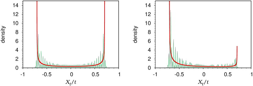
Figure 2: (Color online) Comparison between simulation results and the probability densities of limit distributions for the two-component model. (a) Symmetric and (b) asymmetric cases.

The result (96) with (97) is completely identified with the previous results Kon02 ; Kon05a ; KFK05 . Here we put $(\alpha,\beta,\gamma)=(0,-3\pi/2,\pi)$. Then we have

$$R^{(1/2)}=\frac{{\rm i}}{\sqrt{2}}\left(\begin{array}[]{cc}1&1\cr 1&-1\end{array}\right),$$ (105)

which is the Hadamard matrix multiplied by ${\rm i}$. (Remark that the factor ${\rm i}$ is irrelevant for limit distribution, but by this factor $R^{(1/2)}$ is in SU(2), see KFK05 .) When we choose the initial qubit as ${}^{t}\phi_{0}=(1+{\rm i},1-{\rm i})/2$, the limit distribution of pseudovelocity is symmetric as shown by Fig.2 (a), but when we choose ${}^{t}\phi_{0}=(1+{\rm i},1+{\rm i})/2$, only changing the sign of imaginary part of the second component, the limit distribution becomes asymmetric as shown by Fig. 2 (b). When $(\alpha,\beta,\gamma)=(0,-3\pi/2,\pi)$, the former initial qubit satisfies the condition ${\cal M}^{(1/2,1/2)}_{1}=0$, but the latter does not, where ${\cal M}^{(1/2,1/2)}_{1}$ is given by (97). The shape of probability density function in limit distribution is very sensitive to changes of initial qubit.

Three-component model

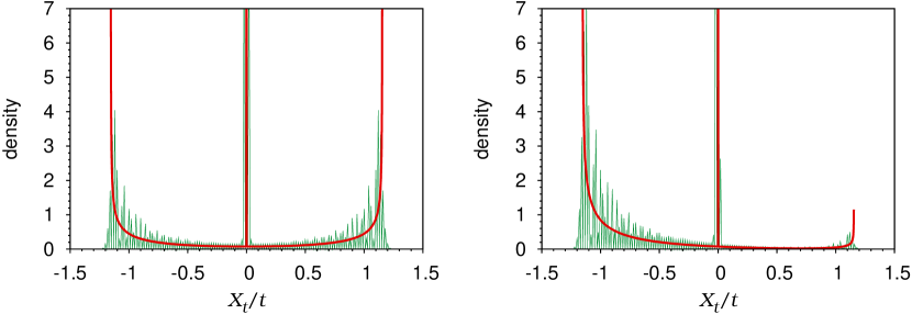
Figure 3: (Color online) Comparison between simulation results and the probability densities of limit distributions for the three-component model. (a) Symmetric and (b) asymmetric cases. The perpendicular thick lines at the origin indicate Dirac’s delta functions.

If we set $(\alpha,\beta,\gamma)=(0,\arccos(-1/3),\pi)$, the three-component quantum coin will be

$$R^{(1)}=\frac{1}{3}\left(\begin{array}[]{ccc}-1&-2&-2\cr-2&-1&2\cr-2&2&-1\end{array}\right).$$ (106)

Remark that it is similar to the Grover matrix Gro97 , but it is not the same. Figure 3 shows the comparison of simulation results and limit distributions for (a) ${}^{t}\phi_{0}=(1-{\rm i},1+{\rm i},1-{\rm i})/\sqrt{6}$, which gives symmetric distribution, and for (b) ${}^{t}\phi_{0}=(1-{\rm i},1-{\rm i},1-{\rm i})/\sqrt{6}$, which gives asymmetric distribution, respectively. It is readily checked that the case (a) satisfies the condition ${\cal M}^{(1,1)}_{1}=0$ for symmetric distribution. In the three-component model, Dirac’s delta-function-type peak at the origin is usually observed in simulation.

Four-component model

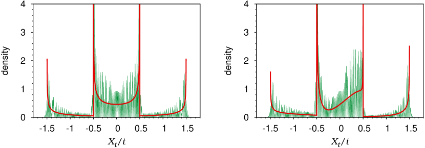
Figure 4: (Color online) Comparison between simulation results and the probability densities of limit distributions for the four-component model. (a) Symmetric and (b) asymmetric cases.

We set $(\alpha,\beta,\gamma)=(0,2\pi/3,\pi)$ for the four-component model, which corresponds to choosing the quantum coin as

$$R^{(3/2)}=\frac{{\rm i}}{8}\left(\begin{array}[]{cccc}1&3&3\sqrt{3}&3\sqrt{3}\cr 3&5&\sqrt{3}&-3\sqrt{3}\cr 3\sqrt{3}&\sqrt{3}&-5&3\cr 3\sqrt{3}&-3\sqrt{3}&3&-1\end{array}\right).$$ (107)

If we assume the initial qudit as

$$\phi_{0}=\frac{1}{2\sqrt{5}}\left(\begin{array}[]{c}1+3{\rm i}\cr 0\cr 0\cr-3+{\rm i}\end{array}\right)\,\mbox{and}\quad\phi_{0}=\frac{1}{2\sqrt{5}}\left(\begin{array}[]{c}1+3{\rm i}\cr 0\cr 0\cr-3-{\rm i}\end{array}\right),$$ (108)

the distributions are determined as shown in Fig. 4 (a) and Fig. 4 (b), respectively.

We observe oscillatory behavior of density functions of $X_{t}/t$ in computer simulations. In general, as the time step $t$ increases, the frequency of oscillation becomes higher. But the convergence of any moments given by (93) means that, if we smear out the oscillatory behavior, the averaged lines of density functions will be well-described by those of the limit distributions (94), which is the fact demonstrated by the above figures.

Now we discuss relations between our models and other multi-component models and possible future problems. Inui and Konno IK05 and Inui et al. IKS05 introduced a one-dimensional three-component quantum walk and showed that a kind of localization phenomenon occurs in their model by calculating the long-time distribution of walker’s position $X_{t}$. They claimed that such a localization phenomenon results in a point mass at the origin, represented by Dirac’s delta function, in the limit distribution of $X_{t}/t$. Though their model associated with the Grover matrix does not belong to our family of models, the structure of probability density function in limit distribution obtained in our three-component model ($j=1$ case) (94) with $j=m=1$ and with (98) is very similar to the limit density function of $X_{t}/t$, given by Eq.(16) in IKS05 . Then the present work suggests that such a localization phenomenon is universal for the models, in which there is a positive probability for walker to stay at the same position in each step. Further study of localization phenomena in quantum-walk models will be an interesting future problem. The relation between the present models and the tensor-product models of Brun et al. BCA03 was already discussed in Sec.IV. Similarity between the density functions of walkers plotted in Fig.1 in their paper and ours shown above will be explained by reducibility of tensor-product models. As demonstrated in Sec.IV. C, their $2^{2}$-dimensional model will include our three-component model and their $2^{3}$-dimensional model does our four-component one, and thus the density function shown by Fig.1(b) (resp. Fig.1(c)) of Brun et al. BCA03 has the same structure with Fig.3(b) (resp. Fig.4(b)) in the present paper. Venegas-Andraca et al. VBBB05 also reported quantum-walk models with entangle coins, where a variety of distributions of walker’s position with multi-peak zones are plotted in figures. They constructed quantum coins for multi-component qudits by also considering tensor products of the basic two-component quantum coins. Systematic classifications of multi-component quantum-walk models and patterns of their limit distributions will be an important future problem. In the present paper, we gave the explicit expressions of ${\cal M}^{(j,m)}(x)$ for $j=1/2,1$ and $3/2$. Here we gave only key formulas in Appendix C for calculation of them, but the present result implies that ${\cal M}^{(j,m)}(x)$ are generally given by polynomials. We hope that further study of ${\cal M}^{(j,m)}$ is a promising subject in the field of quantum walks. As reported in GJS04 ; MBSS02 ; Ken06 ; IKK04 ; GJS05 ; VBBB05 , multi-component models have been studied to simulate quantum walks on the plane, in the higher-dimensional lattices ${\bf Z}^{d}$, or on general graphs. The present work suggests that the group-theoretical investigation will be useful to perform systematic study of such extended models of quantum walks and quantum processes.

Appendix A The matrices $r^{(j)}(\beta)$ for $j=1/2,1,3/2$

The explicit expressions of $r^{(j)}(\beta)$ are readily derived from the Wigner formula (7) as follows for $j=1/2,1,3/2$. Let $c=\cos(\beta/2),s=\sin(\beta/2).$ Then

$$r^{(1/2)}(\beta) = \left(\begin{array}[]{cc}c&-s\cr s&c\end{array}\right),$$ (111)

$$r^{(1)}(\beta) = \left(\begin{array}[]{ccc}c^{2}&-\sqrt{2}cs&s^{2}\cr\sqrt{2}cs&2c^{2}-1&-\sqrt{2}cs\cr s^{2}&\sqrt{2}cs&c^{2}\end{array}\right),$$ (115)

$$r^{(3/2)}(\beta)$$ (120)

$$= \left(\begin{array}[]{llll}c^{3}&-\sqrt{3}c^{2}s&\sqrt{3}cs^{2}&-s^{3}\cr\sqrt{3}c^{2}s&-2cs^{2}+c^{3}&s^{3}-2c^{2}s&\sqrt{3}cs^{2}\cr\sqrt{3}cs^{2}&-s^{3}+2c^{2}s&-2cs^{2}+c^{3}&-\sqrt{3}c^{2}s\cr s^{3}&\sqrt{3}cs^{2}&\sqrt{3}c^{2}s&c^{3}\end{array}\right).$$

Appendix B PROOF OF EQUATIONS (60) WITH (61)

By (16), it is enough to prove the equality

$$R^{(j)}(\alpha,\beta,\gamma)=R^{(j)}(\phi,\theta,0)R^{(j)}(-p,0,0)[R^{(j)}(\phi,\theta,0)]^{\dagger}$$ (122)

with relations

$$\frac{1}{2}(\alpha-\gamma)=\phi+\frac{\pi}{2},\quad\tan\frac{1}{2}(\alpha+\gamma)=-\tan\frac{p}{2}\cos\theta,\quad\sin\frac{\beta}{2}=\sin\frac{p}{2}\sin\theta.$$ (123)

The equality (122) is a matrix representation of the equality which will hold among the rotations

$$\hat{R}(\alpha,\beta,\gamma)=\hat{R}(\phi,\theta,0)\hat{R}(-p,0,0)[\hat{R}(\phi,\theta,0)]^{\dagger}.$$ (124)

Since rotation matrices defined by (5) with $j=1/2,1,3/2,\cdots$ are faithful representations of rotations, it may be enough to prove the equality (122) for the simplest case, $j=1/2$, since it implies (124). By direct calculation, we have

$$R^{(1/2)}(\phi,\theta,0)R^{(1/2)}(-p,0,0)[R^{(1/2)}(\phi,\theta,0)]^{\dagger}$$ (131)

$$= \left(\begin{array}[]{cc}e^{-{\rm i}\phi/2}\cos(\theta/2)&-e^{-{\rm i}\phi/2}\sin(\theta/2)\cr e^{{\rm i}\phi/2}\sin(\theta/2)&e^{{\rm i}\phi/2}\cos(\theta/2)\end{array}\right)\left(\begin{array}[]{cc}e^{{\rm i}p/2}&0\cr 0&e^{-{\rm i}p/2}\end{array}\right)\left(\begin{array}[]{cc}e^{{\rm i}\phi/2}\cos(\theta/2)&e^{-{\rm i}\phi/2}\sin(\theta/2)\cr-e^{{\rm i}\phi/2}\sin(\theta/2)&e^{-{\rm i}\phi/2}\cos(\theta/2)\end{array}\right)$$

$$= \left(\begin{array}[]{cc}\cos(p/2)+{\rm i}\sin(p/2)\cos\theta&{\rm i}\sin(p/2)\sin\theta e^{-{\rm i}\phi}\cr{\rm i}\sin(p/2)\sin\theta e^{{\rm i}\phi}&\cos(p/2)-{\rm i}\sin(p/2)\cos\theta\end{array}\right).$$ (134)

Comparing it with

$$R^{(1/2)}(\alpha,\beta,\gamma)=\left(\begin{array}[]{cc}e^{-{\rm i}(\alpha+\gamma)/2}\cos(\beta/2)&-e^{-{\rm i}(\alpha-\gamma)/2}\sin(\beta/2)\cr e^{{\rm i}(\alpha-\gamma)/2}\sin(\beta/2)&e^{{\rm i}(\alpha+\gamma)/2}\cos(\beta/2)\end{array}\right),$$

we have the equations

$$\cos\frac{p}{2}=\cos\frac{\beta}{2}\cos\frac{1}{2}(\alpha+\gamma),\quad\sin\frac{p}{2}\cos\theta=-\cos\frac{\beta}{2}\sin\frac{1}{2}(\alpha+\gamma),$$

$$\sin\frac{p}{2}\sin\theta\sin\phi=-\sin\frac{\beta}{2}\cos\frac{1}{2}(\alpha-\gamma),\quad\sin\frac{p}{2}\sin\theta\cos\phi=\sin\frac{\beta}{2}\sin\frac{1}{2}(\alpha-\gamma),$$ (136)

from which (123) is derived.

Appendix C FORMULAS

Inserting (6) with (7) into (68) and taking square of the complex variable, we have the expression

$$|C_{m}^{(j)}(k)|^{2} = \sum_{m_{1}=-j}^{j}\sum_{m_{2}=-j}^{j}q_{m_{1}}\overline{q}_{m_{2}}e^{{\rm i}(m_{1}-m_{2})\phi(k)}\sum_{\ell_{1}}\sum_{\ell_{2}}\Gamma(j,m_{1},m,\ell_{1})\Gamma(j,m_{2},m,\ell_{2})$$ (137)

$$\qquad\times\left(\cos\frac{\theta(k)}{2}\right)^{4j+m_{1}+m_{2}-2m-2\ell_{1}-2\ell_{2}}\left(\sin\frac{\theta(k)}{2}\right)^{2\ell_{1}+2\ell_{2}+2m-m_{1}-m_{2}}.$$

From (LABEL:eqn:mapA3)-(74), the following relations are derived,

$$\cos\theta(k)=-\cos\frac{\beta}{2}\sin\chi,$$

$$\sin\theta(k)e^{{\rm i}\phi(k)}=\left(\sin\frac{\beta}{2}\sin\chi-{\rm i}\cos\chi\right)e^{-{\rm i}\gamma}.$$ (138)

Then, through the change of variable (86), we have

$$\cos^{2}\frac{\theta(k)}{2} = \frac{1}{2}\left(1-\frac{y}{2m}\right),$$

$$\sin^{2}\frac{\theta(k)}{2} = \frac{1}{2}\left(1+\frac{y}{2m}\right),$$

$$\sin\frac{\theta(k)}{2}\cos\frac{\theta(k)}{2}e^{{\rm i}\phi(k)} = \frac{1}{2}\left\{\frac{y}{2m}\tan\frac{\beta}{2}-{\rm i}\sqrt{1-\left(\frac{y}{2m}\right)^{2}\sec^{2}\frac{\beta}{2}}\right\}e^{-{\rm i}\gamma}.$$ (139)

By (139) we can perform the transformations $|C^{(j)}_{m}(k)|^{2}\mapsto|\hat{C}^{(j)}_{m}(\chi)|^{2}\mapsto|c^{(j)}_{m}(y)|^{2}$, and ${\cal M}^{(j,m)}(y/2m)$’s are obtained.

In order to calculate (100), we have used the following integral formulas,

$$\int_{0}^{2\cos(\beta/2)}\frac{1}{\sqrt{\cos^{2}(\beta/2)-(y/2)^{2}}}dy = \pi,$$

$$\int_{0}^{2\cos(\beta/2)}\frac{1}{\{1-(y/2)^{2}\}\sqrt{\cos^{2}(\beta/2)-(y/2)^{2}}}dy = \frac{\pi}{\sin(\beta/2)}.$$ (140)

References

- (1) F. Reif, Fundamentals of Statistical and Thermal Physics (McGraw-Hill, New York, 1965).
- (2) N. G. van Kampen, Stochastic Processes in Physics and Chemistry (North-Holland, Amsterdam, 1992).
- (3) R. Motwani and P. Raghavan, Randomized Algorithms (Cambridge University Press, Cambridge, 1995).
- (4) Y. Aharonov, L. Davidovich, and N. Zagury, Phys. Rev. A 48, 1687 (1993).
- (5) D. A. Meyer, J. Stat. Phys. 85, 551 (1996).
- (6) A. Nayak and A. Vishwanath, e-print quant-ph/0010117.
- (7) A. Ambainis, E. Bach, A. Nayak, A. Vishwanath, and J. Watrous, in Proceedings of the 33rd Annual ACM Symposium on Theory of Computing (ACM Press, New York, 2001), pp.37-49.
- (8) T. Oka, N. Konno, R. Arita, and H. Aoki, Phys. Rev. Lett. 94, 100602 (2005).
- (9) N. Konno, Quantum Inf. Process 1, 345 (2002).
- (10) N. Konno, J. Math. Soc. Jpn, 57, 1179 (2005).
- (11) G. Grimmett, S. Janson, and P. F. Scudo, Phys. Rev. E 69, 026119 (2004).
- (12) L. K. Grover, Phys. Rev. Lett. 79, 325 (1997).
- (13) A. Ambainis, in Proc. 45th Annual IEEE Symp. on Foundations of Computer Science (Piscataway, NJ, IEEE, 2004), pp.22-31.
- (14) J. Kempe, Contemp. Phys. 44, 307 (2003).
- (15) B. Tregenna, W. Flanagan, W. Maile, and V. Kendon, New J. Phys. 5, 83 (2003).
- (16) A. Ambainis, Int. J. Quantum Inf. 1, 507 (2003).
- (17) T. D. Mackay, S. D. Bartlett, L. T. Stephenson, and B. C. Sanders, J. Phys. A: Math. Gen. 35, 2745 (2002).
- (18) T. A. Brun, H. A. Carteret, and A. Ambainis, Phys. Rev. A 67, 052317 (2003).
- (19) V. M. Kendon, Int. J. Quantum Inf. 4, 791 (2006).
- (20) N. Konno, Fluct. Noise Lett. 5, L529 (2005).
- (21) A. D. Gottlieb, S. Janson, and P. F. Scudo, Inf. Dim. Anal. Quantum Probab. Rel. Topics, 8, 129 (2005).
- (22) N. Konno, Inf. Dim. Anal. Quantum Probab. Rel. Topics, 9, 287 (2006).
- (23) N. Obata, Inf. Dim. Anal. Quantum Probab. Rel. Topics, 9, 299 (2006).
- (24) N. Konno, Quantum Walks, Lecture at the School “Quantum Potential Theory: Structure and Applications to Physics” held at the Alfried Krupp Wissenschaftskolleg, Greifswald, 26 February - 9 March 2007. (Reihe Mathematik, Ernst-Moritz-Arndt-Universität Greifswald, No.2, 2007.)
- (25) M. Katori, S. Fujino, and N. Konno, Phys. Rev. A 72, 012316 (2005).
- (26) N. Konno, e-print quant-ph/0310191.
- (27) A. J. Bracken, D. Ellinas, and I. Smyrnakis, Phys. Rev. A 75, 022322 (2007).
- (28) H. Georgi, Lie Algebras in Particle Physics, 2nd ed. (Perseus Books, Reading, 1999).
- (29) T. A. Brun, H. A. Carteret, and A. Ambainis, Phys. Rev. Lett. 91, 130602 (2003).
- (30) S. E. Venegas-Andraca, J. L. Ball, K. Burnett, and S. Bose, New J. Phys. 7, 221 (2005).
- (31) A. Messiah, Quantum mechanics, vol. II, (North Holland, Amsterdam, 1962).
- (32) E. P. Wigner, Group Theory and Its Application to the Quantum Mechanics of Atomic Spectra (Academic Press, New York, 1959).
- (33) N. Inui and N. Konno, Physica A 353, 133 (2005).
- (34) N. Inui, N. Konno and E. Segawa, Phys. Rev. E 72, 056112 (2005).
- (35) N. Inui, Y. Konishi, and N. Konno, Phys. Rev. A 69, 052323 (2004).