Merlin-Arthur Games and Stoquastic Complexity

Abstract

$\mathrm{MA}$ is a class of decision problems for which ‘yes’-instances have a proof that can be efficiently checked by a classical randomized algorithm. We prove that $\mathrm{MA}$ has a natural complete problem which we call the stoquastic $k$-SAT problem. This is a matrix-valued analogue of the satisfiability problem in which clauses are $k$-qubit projectors with non-negative matrix elements, while a satisfying assignment is a vector that belongs to the space spanned by these projectors. Stoquastic $k$-SAT is the first non-trivial example of a $\mathrm{MA}$-complete problem. We also study the minimum eigenvalue problem for local stoquastic Hamiltonians that was introduced in Ref. [1], stoquastic LH-MIN. A new complexity class $\mathrm{StoqMA}$ is introduced so that stoquastic LH-MIN is $\mathrm{StoqMA}$-complete. We show that $\mathrm{MA}{}\subseteq\mathrm{StoqMA}{}\subseteq{\rm SBP}\cap{\rm QMA}$. Lastly, we consider the average LH-MIN problem for local stoquastic Hamiltonians that depend on a random or ‘quenched disorder’ parameter, stoquastic AV-LH-MIN. We prove that stoquastic AV-LH-MIN is contained in the complexity class $\mathrm{AM}$, the class of decision problems for which yes-instances have a randomized interactive proof with two-way communication between prover and verifier.

1 Introduction

Recent years have seen the first steps in the development of a quantum or matrix-valued complexity theory. Such complexity theory is interesting for a variety of reasons. Firstly, as in the classical case it may increase our understanding of the power and limitations of quantum computation. Secondly, since quantum computation is an extension of classical computation, this complexity theory provides a framework and new angle from which we can view classical computation.

In this paper we will provide such a new point of view for the complexity class $\mathrm{MA}$ defined by Babai [2]. We do this by studying so-called stoquastic problems, first defined in [1]. The first problem we consider is one that arises naturally through a quantum or matrix-valued generalization of the satisfiability problem [3]. The input of quantum $k$-SAT is a tuple $(n,\epsilon,\Pi_{1},\ldots,\Pi_{M},S_{1},\ldots,S_{M})$, where $n$ is a number of qubits, $\epsilon\geq n^{-O(1)}$ is a precision parameter, and $\Pi_{1},\ldots,\Pi_{M}$ are Hermitian projectors acting on the Hilbert space of $n$ qubits. Each projector $\Pi_{\alpha}$ acts non-trivially only on some subset of $k$ qubits $S_{\alpha}\subseteq\{1,2,\ldots,n\}$. Then the promise problem quantum $k$-SAT is stated as follows:

• yes-instance: There exists a state $|\theta\rangle\in(\mathbb{C}^{2})^{\otimes n}$ such that for all $\alpha=1,\ldots,M$, $\Pi_{\alpha}\,|\theta\rangle=|\theta\rangle$.

• no-instance: For any state $|\theta\rangle\in(\mathbb{C}^{2})^{\otimes n}$ there is some $\alpha\in\{1,\ldots,M\}$ such that $\langle\theta|\Pi_{\alpha}|\theta\rangle\leq 1-\epsilon$.

(Here a state is a vector $|\theta\rangle\in(\mathbb{C}^{2})^{\otimes n}$ with a unit norm $\langle\theta|\theta\rangle=1$.) A state $|\theta\rangle$ satisfying the condition for a yes-instance is called a solution, or a satisfying assignment.

If the projectors $\Pi_{\alpha}$ have zero off-diagonal elements in the computational basis, a solution $|\theta\rangle$ can always be chosen as a basis vector, $|\theta\rangle=|x\rangle$, $x\in\{0,1\}^{n}$. In this case quantum $k$-SAT reduces to classical $k$-SAT which is known to be $\mathrm{NP}$-complete for $k\geq 3$. On the other hand, if no restrictions on the matrix elements of $\Pi_{\alpha}$ are imposed, quantum $k$-SAT is complete for Quantum $\mathrm{MA}$, or $\mathrm{QMA}$, defined by Kitaev [6, 10] if $k\geq 4$, see [3]. The class $\mathrm{QMA}$ has been extensively studied in [7, 8, 9, 10, 11, 12, 13, 14, 15]. It was proved that quantum $2$-SAT has an efficient classical algorithm [3] similar to classical $2$-SAT.

Let us now properly define the restriction that defines the stoquastic $k$-SAT problem:

Definition 1.

Stoquastic $k$-SAT is defined as quantum $k$-SAT with the restriction that all projectors $\Pi_{\alpha}$ have real non-negative matrix elements in the computational basis.

The term ‘stoquastic’ was introduced in Ref. [1] to suggest the relation both with stochastic processes and quantum operators. We will show that

Theorem 1.

Stoquastic $k$-SAT is contained in $\mathrm{MA}$ for any constant $k$ and $\mathrm{MA}$-hard for $k\geq 6$.

It follows that stoquastic $6$-SAT is $\mathrm{MA}$-complete. This is the first known example of a natural $\mathrm{MA}$-complete problem. The proof of the theorem involves a novel polynomial-time random-walk-type algorithm that takes as input an instance of stoquastic $k$-SAT and a binary string $x\in\{0,1\}^{n}$. The algorithm checks whether there exists a solution $|\theta\rangle$ having large enough overlap with the basis vector $|x\rangle$. Description of such a basis vector can serve as a proof that a solution exists. The proof of Theorem 1 is given in Section 3.1.

Our second result concerns the complexity class $\mathrm{AM}$ (Arthur-Merlin games). $\mathrm{AM}$ is a class of decision problems for which ‘yes’-instances have a randomized interactive proof with a constant number of communication rounds between verifier Arthur and prover Merlin. By definition, $\mathrm{MA}{}\subseteq\mathrm{AM}$. It was shown that $\mathrm{AM}$ contains some group theoretic problems [2], the graph non-isomorphism problem [16] and the approximate set size problem [5]. We show that there exists an interesting quantum mechanical problem that is in $\mathrm{AM}$ (and in fact $\mathrm{AM}$-complete). It is closely related to the minimum eigenvalue problem for a local Hamiltonian [6] which we shall abbreviate as LH-MIN. The input of LH-MIN is a tuple $(n,H_{1},\ldots,H_{M},S_{1},\ldots,S_{M},\lambda_{\mbox{\small\it yes}},\lambda_{\mbox{\small\it no}})$, where $n$ is the total number of qubits, $H_{\alpha}$ is a Hermitian operator on $n$ qubits acting non-trivially only on a subset of $k$ qubits $S_{\alpha}\subseteq\{1,2,\ldots,n\}$, and $\lambda_{\mbox{\small\it yes}}<\lambda_{\mbox{\small\it no}}$ are real numbers. It is required that $||H_{\alpha}||\leq n^{O(1)}$ and $\lambda_{\mbox{\small\it no}}-\lambda_{\mbox{\small\it yes}}\geq n^{-O(1)}$. The promise problem LH-MIN is stated as follows:

• yes-instance: There exists a state $|\theta\rangle\in(\mathbb{C}^{2})^{\otimes n}$ such that $\sum_{\alpha=1}^{M}\langle\theta|H_{\alpha}|\theta\rangle\leq\lambda_{\mbox{\small\it yes}}$.

• no-instance: For any state $|\theta\rangle\in(\mathbb{C}^{2})^{\otimes n}$ one has $\sum_{\alpha=1}^{M}\langle\theta|H_{\alpha}|\theta\rangle\geq\lambda_{\mbox{\small\it no}}$.

In other words, the minimum eigenvalue $\lambda(H)$ of a $k$-local Hamiltonian $H=\sum_{\alpha}H_{\alpha}$ obeys $\lambda(H)\leq\lambda_{\mbox{\small\it yes}}$ for yes-instances and $\lambda(H)\geq\lambda_{\mbox{\small\it no}}$ for no-instances.

LH-MIN for 2-local Hamiltonians can be viewed as the natural matrix-valued generalization of MAX2SAT which is the problem of determining the maximum number of satisfied clauses where each clause has two variables. It was shown in [6, 10] that LH-MIN is $\mathrm{QMA}$-complete for $k\geq 2$. The authors in Ref. [1] considered the LH-MIN problem for so-called stoquastic Hamiltonians.

Definition 2.

Stoquastic LH-MIN is defined as LH-MIN with the restriction that all operators $H_{\alpha}$ have real non-positive off-diagonal matrix elements in the computational basis.

The important consequence of this restriction is that the eigenvector with lowest eigenvalue, also called the ground-state, of a Hamiltonian $H=\sum_{\alpha}H_{\alpha}$ is a vector with nonnegative coefficients in the computational basis. This allows for an interpretation of this vector as a probability distribution. For a general Hamiltonian the ground-state is a vector with complex coefficients for which no such representation exists. Besides, stoquastic $k$-SAT is a special case of $k$-local stoquastic LH-MIN (choose $\Pi_{\alpha}$ as a projector onto the space on which $H_{\alpha}$ takes its smallest eigenvalue $\lambda_{\alpha}$ and choose $\lambda_{\mbox{\small\it yes}}=\sum_{\alpha}\lambda_{\alpha}$). The authors in Ref. [1] have proved that (i) the complexity of stoquastic LH-MIN does not depend on the locality parameter $k$ if $k\geq 2$; (ii) stoquastic LH-MIN is hard for $\mathrm{MA}$; (iii) stoquastic LH-MIN is contained in any of the complexity classes $\mathrm{QMA}$, $\mathrm{AM}$, $\mathrm{PostBPP}$ (the latter inclusion was proved only for Hamiltonians with polynomial spectral gap), where $\mathrm{PostBPP}$=$\mathrm{BPP_{path}}$, see [1, 18].

In the present paper we formulate a random stoquastic LH-MIN problem that we prove to be complete for the class $\mathrm{AM}$. In fact the most interesting aspect of this result is that this problem is contained in $\mathrm{AM}$, since it is not hard to formulate a complete problem for $\mathrm{AM}$, see below. Let us define this problem stoquastic AV-LH-MIN properly. We consider an ensemble of local stoquastic Hamiltonians $\{H(r)\}$ for which $r$ is a string of $m=n^{O(1)}$ bits, and $r$ is taken from the uniform distribution on $\Sigma^{m}$. Such a random ensemble $\{H(r)\}$ is called $(k,l)$-local if $H(r)$ can be written as $H(r)=\sum_{\alpha=1}^{M}H_{\alpha}(r),\quad M=n^{O(1)}$, where $H_{\alpha}(r)$ is a Hermitian operator on $n$ qubits acting non-trivially only on some subset of qubits $S_{\alpha}\subseteq\{1,\ldots,n\}$, $|S_{\alpha}|\leq k$. Furthermore, $H_{\alpha}(r)$ depends only on some subset of random bits $R_{\alpha}\subseteq\{1,\ldots,m\}$, $|R_{\alpha}|\leq l$. We will consider ensembles in which the Hamiltonians $H(r)$ are stoquastic, i.e. each $H_{\alpha}(r)$ has real non-positive off-diagonal matrix elements for all $r$ . The input of the problem stoquastic AV-LH-MIN involves a description of a $(k,l)$-local stoquastic ensemble $\{H(r)\}$ on $n$ qubits and $m$ random bits, and two thresholds $\lambda_{\mbox{\small\it yes}}<\lambda_{\mbox{\small\it no}}$. It is required that $||H_{\alpha}(r)||\leq n^{O(1)}$ for all $r$, and $\lambda_{\mbox{\small\it no}}-\lambda_{\mbox{\small\it yes}}\geq n^{-O(1)}$. Let us denote by $\lambda(r)$ the smallest eigenvalue of $H(r)$ and $\bar{\lambda}=2^{-m}\sum_{r\in\Sigma^{m}}\lambda(r)$ the average value of $\lambda(r)$. The stoquastic AV-LH-MIN problem is to decide whether $\bar{\lambda}\leq\lambda_{\mbox{\small\it yes}}$ (a yes-instance) or $\bar{\lambda}\geq\lambda_{\mbox{\small\it no}}$ (a no-instance). Our second result is

Theorem 2.

Stoquastic AV-LH-MIN is contained in $\mathrm{AM}$ for any $k,l=O(1)$. Stoquastic $(3,1)$-local AV-LH-MIN is AM-complete.

The proof of the theorem is presented in Section 5. It should be mentioned that the stoquastic $(3,1)$-local ensemble $\{H(r)\}$ corresponding to $\mathrm{AM}$-hard problem in Theorem 2 is actually an ensemble of classical $3$-SAT problems, that is, for each random string $r$ all operators $H_{\alpha}(r)$ in the decomposition $H(r)=\sum_{\alpha}H_{\alpha}(r)$ are projectors diagonal in the computational basis. For yes-instance of the problem one has $\lambda(r)=0$ for all $r$ (and thus $\bar{\lambda}=0$), while for no-instances $\lambda(r)=0$ with probability at most $1/3$ (and thus $\bar{\lambda}\geq 2/3$), see Section 5. Since classical $3$-SAT is a special case of stoquastic $3$-SAT, we conclude that a $(3,1)$-local ensemble of stoquastic $3$-SAT problems also yields an $\mathrm{AM}$-complete problem.

Our final result concerns the complexity of stoquastic LH-MIN (without disorder). We define a new complexity class $\mathrm{StoqMA}$ which sits between $\mathrm{MA}$ and $\mathrm{QMA}$ and we prove, see Section 4, that

Theorem 3.

Stoquastic $k$-local LH-MIN is $\mathrm{StoqMA}$-complete for any $k\geq 2$.

The class $\mathrm{StoqMA}$ is a restricted version of $\mathrm{QMA}$ in which the verifier can perform only classical reversible gates, prepare qubits in $|0\rangle$ and $|+\rangle$ states, and perform one measurement in the $|+\rangle,|-\rangle$ basis. This results solves the open problem posed in [1] concerning the complexity of stoquastic LH-MIN. We also establish some relations between $\mathrm{StoqMA}$ and already known complexity classes. Ref. [17] introduced a complexity class $\mathrm{SBP}$ (Small Bounded-Error Probability) as a natural class sitting between $\mathrm{MA}$ and $\mathrm{AM}$. We prove that stoquastic LH-MIN and thus all of $\mathrm{StoqMA}$ is contained in $\mathrm{SBP}$, see Section 4.1.1 for details. Figure 1 illustrates the relevant complexity classes and their inter-relations.

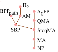
Figure 1: Inclusion tree for the relevant complexity classes. Here $\mathrm{BPP_{path}}$=$\mathrm{PostBPP}$.

In conclusion, our results show that the randomized versions of stoquastic LH-MIN, stoquastic $k$-SAT and classical $k$-SAT are of equal complexity, that is they are all $\mathrm{AM}$-complete. On the other hand, it is at present unclear whether the original problems (not randomized) $k$-SAT, stoquastic $k$-SAT and stoquastic LH-MIN and thus the corresponding classes $\mathrm{NP}$, $\mathrm{MA}$ and $\mathrm{StoqMA}$ are of equal complexity. We would like to note that any proof of a separation between $\mathrm{MA}$ and $\mathrm{AM}$ (for example via a separation of $\mathrm{MA}$ and $\mathrm{StoqMA}$) would have far-reaching consequences. Namely it was proved in [21] that

Theorem 4 ([21]).

If $\mathrm{MA}{}\neq\mathrm{AM}{}$ then $\mathrm{NP}{}\not\subseteq\mathrm{P}{}/{\rm poly}$.

2 Definitions of relevant complexity classes

Throughout the paper $\Sigma^{n}$ and $\Sigma^{*}$ will denote a set of $n$-bit strings and the set of all finite bit strings respectively.

Definition 3 ($\mathrm{MA}$).

A promise problem $L=L_{\mbox{\small\it yes}}\cup L_{\mbox{\small\it no}}\subseteq\Sigma^{*}$ belongs to $\mathrm{MA}$ iff there exist a polynomial $p(n)$ and a $\mathrm{BPP}$ predicate $V(x,w)$ such that

$$x\in L_{\mbox{\small\it yes}} \Rightarrow \exists\,w\quad{\bf Pr}{\left[V(x,w)=1\right]}\geq 2/3\;\;\mbox{\rm(Completeness)}$$

$$x\in L_{\mbox{\small\it no}} \Rightarrow \forall\,w\quad{\bf Pr}{\left[V(x,w)=1\right]}\leq 1/3\;\;\mbox{\rm(Soundness)}$$

Here $x\in\Sigma^{*}$ represents the instance of a problem and $w\in\Sigma^{p(|x|)}$ represents the prover’s witness string. If an instance $x$ does not satisfy the promise, i.e., $x\notin L_{\mbox{\small\it yes}}\cup L_{\mbox{\small\it no}}$, then $V(x,w)$ may be arbitrary (or even undefined).

In [1] it was proved that $\mathrm{MA}$ has an alternative quantum-mechanical definition as a restricted version of $\mathrm{QMA}$ in which the verifier is a coherent classical computer, see the review in Section A.3 of the Appendix. $\mathrm{StoqMA}$ is a class of decision problems for which the answer ‘yes’ has a short quantum certificate that can be efficiently checked by a stoquastic verifier:

Definition 4 ($\mathrm{StoqMA}$).

A stoquastic verifier is a tuple $V=(n,n_{w},n_{0},n_{+},U)$, where $n$ is the number of input bits, $n_{w}$ the number of input witness qubits, $n_{0}$ the number of input ancillas $|0\rangle$, $n_{+}$ the number of input ancillas $|+\rangle$ and $U$ is a quantum circuit on $n+n_{w}+n_{0}+n_{+}$ qubits with $X$, CNOT, and Toffoli gates. The acceptance probability of a stoquastic verifier $V$ on input string $x\in\Sigma^{n}$ and witness state $|\psi\rangle\in(\mathbb{C}^{2})^{\otimes n_{w}}$ is defined as ${\bf Pr}(V;x,\psi)=\langle\psi_{in}|U^{\dagger}\,\Pi_{out}\,U|\psi_{in}\rangle$. Here $|\psi_{in}\rangle=|x\rangle\otimes|\psi\rangle\otimes|0\rangle^{\otimes n_{0}}\otimes|+\rangle^{\otimes n_{+}}$ is the initial state and $\Pi_{out}=|+\rangle\langle+|_{1}\otimes I_{else}$ projects the first qubit onto the state $|+\rangle$.
A promise problem $L=L_{\mbox{\small\it yes}}\cup L_{\mbox{\small\it no}}\subseteq\Sigma^{*}$ belongs to $\mathrm{StoqMA}$ iff there exists a uniform family of stoquastic verifiers, such that for any fixed number of input bits $n$ the corresponding verifier $V$ uses at most $n^{O(1)}$ qubits, $n^{O(1)}$ gates, and obeys completeness and soundness conditions:

$$\quad x\in L_{\mbox{\small\it yes}} \Rightarrow \exists\,|\psi\rangle\in(\mathbb{C}^{2})^{\otimes n_{w}}\quad{\bf Pr}(V;x,\psi)\geq\epsilon_{\mbox{\small\it yes}}\;\;\mbox{\rm(Completeness)}$$

$$\quad x\in L_{\mbox{\small\it no}} \Rightarrow \forall\,|\psi\rangle\in(\mathbb{C}^{2})^{\otimes n_{w}}\quad{\bf Pr}(V;x,\psi)\leq\epsilon_{\mbox{\small\it no}}\;\;\mbox{\rm(Soundness)}$$

Here the threshold probabilities $0\leq\epsilon_{\mbox{\small\it no}}<\epsilon_{\mbox{\small\it yes}}\leq 1$ must have polynomial separation: $\epsilon_{\mbox{\small\it yes}}-\epsilon_{\mbox{\small\it no}}\geq n^{-O(1)}$.

Comments: In contrast to the standard classes $\mathrm{BPP}$, $\mathrm{MA}$, or $\mathrm{QMA}$ the class $\mathrm{StoqMA}$ does not permit amplification of the gap between the threshold probabilities $\epsilon_{\mbox{\small\it no}}$, $\epsilon_{\mbox{\small\it yes}}$ based on majority voting. In fact, it is not hard to show that the state $\psi$ maximizing the acceptance probability has non-negative amplitudes in the computational basis, and ${\bf Pr}(V;x,\psi)\in[\frac{1}{2},1]$ for any non-negative state $|\psi\rangle$.

It is important to note that the only difference between $\mathrm{StoqMA}$ and $\mathrm{MA}$ is that a stoquastic verifier in $\mathrm{StoqMA}$ is allowed to do the final measurement in the $\{|+\rangle,|-\rangle\}$ basis, whereas a classical coherent verifier in $\mathrm{MA}$ can only do a measurement in the standard basis $\{\big{|}0\big{>},\big{|}1\big{>}\}$.

The complexity class $\mathrm{AM}$ was introduced by Babai [2] as a class of decision problems for which the answer ‘yes’ possesses a randomized interactive proof (Arthur-Merlin game) with two-way communication between a prover and a verifier. Babai also showed in [2] that any language in $\mathrm{AM}$ has a proving protocol such that (i) verifier sends prover a uniform random bit string $q$; (ii) prover replies with a witness string $w$; (iii) verifier performs polynomial-time deterministic computation on $q$ and $w$ to decide whether he accepts the proof. Here is a formal definition:

Definition 5 ($\mathrm{AM}$).

A promise problem $L=L_{\mbox{\small\it yes}}\cup L_{\mbox{\small\it no}}\subseteq\Sigma^{*}$ belongs to the class $\mathrm{AM}$ iff there exists a polynomial $p$ and a $\mathrm{P}$ predicate $V(x,q,w)$ defined for any $q,w\in\Sigma^{p(|x|)}$, such that

$$x\in L_{\mbox{\small\it yes}} \Rightarrow {\bf Pr}{\left[\exists\,w\,:\,V(x,q,w)=1\right]}\geq 2/3\;\;\mbox{\rm(Completeness)}$$

$$x\in L_{\mbox{\small\it no}} \Rightarrow {\bf Pr}{\left[\exists\,w\,:\,V(x,q,w)=1\right]}\leq 1/3\;\;\mbox{\rm(Soundness)}$$

where $q\in\Sigma^{p(|x|)}$ is a uniformly distributed random bit string.

Finally, the complexity class $\mathrm{SBP}$ (Small Bounded-error Probability) was introduced in [17] as a natural class sitting between $\mathrm{MA}$ and $\mathrm{AM}$.

Definition 6 ($\mathrm{SBP}$).

A promise problem $L=L_{\mbox{\small\it yes}}\cup L_{\mbox{\small\it no}}\subseteq\Sigma^{*}$ belongs to the class $\mathrm{SBP}$ iff there exists a function $F\in\#$P and a function $f\,:\,\Sigma^{*}\to\mathbb{R}_{+}$ computable in polynomial time such that

$$x\in L_{\mbox{\small\it yes}} \Rightarrow F(x)\geq f(x)\quad\mbox{\rm(Completeness)}$$

$$x\in L_{\mbox{\small\it no}} \Rightarrow F(x)\leq(1/2)\,f(x)\quad\mbox{\rm(Soundness)}$$

It was proved in [17] that $\mathrm{SBP}{}\subseteq\mathrm{AM}{}\cap\mathrm{BPP_{path}}$, where $\mathrm{BPP_{path}}=\mathrm{PostBPP}$, see [1].

3 Stoquastic $6$-SAT is $\mathrm{MA}$-complete

We first argue that stoquastic $k$-SAT is $\mathrm{MA}$-hard for any $k\geq 6$. This result is a simple corollary of Lemma 3 in Ref. [1] which showed that LH-MIN for a 6-local stoquastic Hamiltonian is $\mathrm{MA}$-hard (a more formal proof of this result is also given in Appendix A.3). Indeed, let $L=L_{\mbox{\small\it yes}}\cup L_{\mbox{\small\it no}}$ be any language in $\mathrm{MA}$ and let $V$ be a verifier for this language, see Definition 3. Without loss of generality $V$ accepts with probability $1$ on ‘yes’-instances, see [19]. As was shown in Ref. [1], for every input $x\in L$ one can construct a stoquastic $6$-local Hamiltonian $H=\sum_{\alpha}H_{\alpha}$ such that $\lambda(H)=\lambda_{\mbox{\small\it yes}}=\sum_{\alpha}\lambda(H_{\alpha})$ for $x\in L_{\mbox{\small\it yes}}$ and $\lambda(H)\geq\lambda_{\mbox{\small\it no}}=\lambda_{\mbox{\small\it yes}}+|x|^{-O(1)}$ for $x\in L_{\mbox{\small\it no}}$. The corresponding LH-MIN problem is thus equivalent to quantum $6$-SAT with projectors $\Pi_{\alpha}$ projecting onto the ground-space of $H_{\alpha}$. Such a projector has non-negative matrix elements because $H_{\alpha}$ has non-positive off-diagonal matrix elements. Therefore any problem in $\mathrm{MA}$ can be reduced to stoquastic $6$-SAT:

Corollary 1.

Stoquastic $6$-SAT is $\mathrm{MA}$-hard.

3.1 Stoquastic $k$-SAT is contained in $\mathrm{MA}$

In this section we describe a random-walk-type algorithm for stoquastic $k$-SAT. Given an instance of stoquastic $k$-SAT with the projectors $\{\Pi_{\alpha}\}$ we can define a Hermitian operator

$$G=\frac{1}{M}\sum_{\alpha=1}^{M}\Pi_{\alpha}.$$ (1)

Note also that $G$ has non-negative matrix elements in the computational basis. We have that either the largest eigenvalue of $G$ is $\lambda=1$ (a yes-instance) or $\lambda\leq 1-\epsilon M^{-1}$ (a no-instance) since for any vector $|\theta\rangle$

$$\langle\theta|G|\theta\rangle\leq 1-M^{-1}+M^{-1}\min_{\alpha}\langle\theta|\Pi_{\alpha}|\theta\rangle\leq 1-\epsilon M^{-1}.$$

In order to distinguish $\lambda=1$ and $\lambda\leq 1-\epsilon M^{-1}$ the verifier Arthur will employ a random walk on the space of $n$-bit binary strings. The transition probability from a string $x$ to a string $y$ will be proportional to the matrix element $G_{x,y}$. The role of the prover Merlin is to provide the starting point for the random walk. Each step of the random walk will include a series of tests that are always passed for positive instances. For negative instances the tests are passed with probability strictly less than 1 such that the probability for the random walk to make $L$ steps decreases exponentially with $L$.

In order to illustrate the main idea, we will first define the walk for positive instances only. Suppose that a state

$$|\theta\rangle=\sum_{x\in T}\theta_{x}\,|x\rangle,\quad\theta_{x}>0,\quad T\subseteq\Sigma^{n}$$ (2)

is a satisfying assignment, that is $\Pi_{\alpha}\,|\theta\rangle=|\theta\rangle$ for all $\alpha$. For any binary strings $x,y\in T$ define a transition probability from $x$ to $y$ as

$$P_{x\to y}=G_{x,y}\left(\frac{\theta_{y}}{\theta_{x}}\right),\quad G_{x,y}=\langle x|G|y\rangle.$$ (3)

Clearly, $\sum_{y\in T}P_{x\to y}=1$ for all $x\in T$, so that $P_{x\to y}$ defines a random walk on $T$. A specific feature of solutions of stoquastic $k$-SAT is that the ratio $\theta_{y}/\theta_{x}$ in Eq. (3) can be easily expressed in terms of matrix elements of $\Pi_{\alpha}$, namely one can prove that

Lemma 1.

Assume $\Pi\,:\,\mathbb{C}^{2^{n}}\to\mathbb{C}^{2^{n}}$ is a Hermitian projector having non-negative matrix elements in the computational basis. Assume $\Pi\,|\theta\rangle=|\theta\rangle$ for some state $|\theta\rangle=\sum_{x\in T}\theta_{x}\,|x\rangle$, $\theta_{x}>0$, $T\subseteq\Sigma^{n}$. Then

(1) $\langle x|\Pi|x\rangle>0$ for all $x\in T$,

(2) If $\langle x|\Pi|y\rangle>0$ for some $x,y\in T$ then

$$\frac{\theta_{y}}{\theta_{x}}=\sqrt{\frac{\langle y|\Pi|y\rangle}{\langle x|\Pi|x\rangle}}.$$ (4)

The proof of this lemma can be found in Appendix A.1. Applying the lemma to Eq. (3) we conclude that either $G_{x,y}=P_{x\to y}=0$ or $G_{x,y}>0$ and thus

$$P_{x\to y}=G_{x,y}\,\sqrt{\frac{\langle y|\Pi_{\alpha}|y\rangle}{\langle x|\Pi_{\alpha}|x\rangle}}$$ (5)

for any $\alpha$ such that $\langle y|\Pi_{\alpha}|x\rangle>0$ (since $G_{x,y}>0$ there must exist at least one such $\alpha$). Thus for any fixed $x,y\in T$ we can compute the transition probability $P_{x\to y}$ efficiently. Let, for any fixed $x\in T$, the set of points $y\in T$ that can be reached from $x$ by one step of the random walk be $N(x)=\{y\in\Sigma^{n}\,:\,G_{x,y}>0\}$. This set contains at most $2^{k}\,M=n^{O(1)}$ elements which can be found efficiently since $G$ is a sum of $k$-qubit operators.

Note that definition of transition probabilities Eq. (5) does not explicitly include any information about the solution $|\theta\rangle$. This is exactly the property we are looking for: the definition of the random walk must be the same for positive and negative instances. Of course, applying Eq. (5) to negative instances may produce unnormalized probabilities, such that $\sum_{y\in N(x)}P_{x\to y}$ is either smaller or greater than $1$. Checking normalization of the transition probabilities will be included into the definition of the verifier’s protocol as an extra test. Whenever the verifier observes unnormalized probabilities, he terminates the random walk and outputs ‘reject’. The probability of passing the tests will be related to the largest eigenvalue of $G$. If the verifier performs sufficiently many steps of the walk and all the tests are passed, he gains confidence that the largest eigenvalue of $G$ is $1$. We shall see that the soundness condition in Eq. (3) is fulfilled if the verifier accepts after making $L$ steps of the random walk, where $L$ obeys inequality

$$2^{\frac{n}{2}}\left(1-\frac{\epsilon}{M}\right)^{L}\leq\frac{1}{3}.$$ (6)

Since $\epsilon=n^{-O(1)}$ and the number of clauses $M$ is at most $M\leq{n\choose k}=n^{O(1)}$ one can satisfy this inequality with a polynomial number of steps, $L=n^{O(1)}$. The only step in the definition of the random walk above that can not be done efficiently is choosing the starting point. It requires the prover’s assistance. For reasons related to the soundness of the proof, the prover is required to send the verifier a string $x\in T$ with the largest amplitude $\theta_{x}$.

A formal description of the prover’s strategy is the following. In case of a yes-instance the prover chooses a vector $|\theta\rangle\in(\mathbb{C}^{2})^{\otimes n}$ such that $\Pi_{\alpha}\,|\theta\rangle=|\theta\rangle$ for all $\alpha$. Wlog, $|\theta\rangle$ has positive amplitudes on some set $T\subseteq\Sigma^{n}$, see Eq. (2). The prover sends the verifier a string $w\in T$ such that $\theta_{w}\geq\theta_{x}$ for all $x\in T$. In case of a no-instance the prover may send the verifier an arbitrary string $w\in\Sigma^{n}$.

Here is a formal description of the verifier’s strategy:

Step 1: Receive a string $w\in\Sigma^{n}$ from the prover. Set $x_{0}=w$. Step 2: Suppose the current state of the walk is $x_{j}$. Verify that $\langle x_{j}|\Pi_{\alpha}|x_{j}\rangle>0$ for all $\alpha$. Otherwise reject. Step 3: Find the set $N(x_{j})=\{y\in\Sigma^{n}\,:\,G_{x_{j},y}>0\}$. Step 4: For every $y\in N(x_{j})$ choose any $\alpha=\alpha(y)$ such that $\langle y|\Pi_{\alpha(y)}|x_{j}\rangle>0$. Step 5: For every $y\in N(x_{j})$ compute a number $$P_{x_{j}\to y}=G_{x_{j},y}\,\sqrt{\frac{\langle y|\Pi_{\alpha(y)}|y\rangle}{\langle x_{j}|\Pi_{\alpha(y)}|x_{j}\rangle}}.$$ (7) Step 6: Verify that $\sum_{y\in N(x_{j})}P_{x_{j}\to y}=1$. Otherwise reject. Step 7: If $j=L$ goto Step 10. Step 8: Generate $x_{j+1}\in N(x_{j})$ according to the transition probabilities $P_{x_{j}\to x_{j+1}}$. Step 9: Compute and store a number $$r_{j+1}=\frac{P_{x_{j}\to x_{j+1}}}{G_{x_{j},x_{j+1}}}.$$ (8) Set $j\to j+1$ and goto Step 2. Step 10: Verify that $\prod_{j=1}^{L}r_{j}\leq 1$. Otherwise reject. Step 11: Accept.

Step 4 deserves a comment. It may happen that there are several $\alpha$’s with the property $\langle y|\Pi_{\alpha}|x_{j}\rangle>0$. Let us agree that $\alpha(y)$ is the smallest $\alpha$ satisfying this inequality. In fact, the definition of the transition probabilities $P_{x_{j}\to y}$ should not depend on the choice of $\alpha(y)$ for the yes-instances, see Lemma 1. Step 8 might be impossible to implement exactly when only unbiased random coins are available. This step can be replaced by generating $x_{j+1}$ from a probability distribution $P^{\prime}_{x_{j}\to y}$ which is $\delta$-close in variation distance to $P_{x_{j}\to y}$ for some $\delta=n^{-O(1)}$. This is always possible even with unbiased random coins.

In Appendix A.2 we formally prove the completeness and soundness of this protocol. As a consequence of this and Corollary 1 we obtain Theorem 1.

4 Stoquastic LH-MIN is $\mathrm{StoqMA}$-complete

In this section we will prove Theorem 3.

First we show that stoquastic LH-MIN is contained in $\mathrm{StoqMA}$. Let $H$ be a stoquastic $k$-local Hamiltonian acting on $n$ qubits. It is enough to show that there exist constants $\alpha>0$, $\beta$, and a stoquastic verifier $V$ with $n_{w}=n$ witness qubits, such that

$${\bf Pr}(V;x,\psi)=\langle\psi|\,\left(-\alpha\,H+\beta\,I\right)\,|\psi\rangle\quad\mbox{for all}\quad|\psi\rangle\in(\mathbb{C}^{2})^{\otimes n_{w}},$$ (9)

where $x$ is a classical description of $H$. We shall construct a stoquastic verifier that picks up one local term in $H$ at random and converts this term into an observable proportional to $|+\rangle\langle+|$. This is possible for one particular decomposition of $H$ into local stoquastic terms which we shall describe now.

Lemma 2.

Let $H$ be $k$-local stoquastic Hamiltonian on $n$ qubits. There exist constants $\gamma>0$ and $\beta$ such that

$$\gamma\,H+\beta\,I=\sum_{j}p_{j}\,U_{j}\,H_{j}\,U_{j}^{\dagger},$$ (10)

where $p_{j}\geq 0$, $\sum_{j}p_{j}=1$, $U_{j}$ is a quantum circuit on $n$ qubits with $X$ and CNOT gates. The stoquastic term $H_{j}$ is either $-|0\rangle\langle 0|^{\otimes k}$ or $-X\otimes|0\rangle\langle 0|^{\otimes k-1}$. All terms in the decomposition Eq. (10) can be found efficiently.

The next step is to reduce a measurement of the observables $|0\rangle\langle 0|^{\otimes k}$ and $X\otimes|0\rangle\langle 0|^{\otimes k-1}$ to a measurement of $X$ only.

Lemma 3.

An operator $W\,:\,(\mathbb{C}^{2})^{\otimes p}\to(\mathbb{C}^{2})^{\otimes q}$ is called a stoquastic isometry iff

$$W\,|\psi\rangle=U\,|\psi\rangle\otimes|0\rangle^{\otimes n_{0}}\otimes|+\rangle^{\otimes n_{+}}\quad\mbox{for all}\quad|\psi\rangle\in(\mathbb{C}^{2})^{\otimes p}$$

for some integers $n_{0}$ and $n_{+}$, $q=p+n_{0}+n_{+}$, and some quantum circuit $U$ on $q$ qubits with $X$, CNOT, and Toffoli gates. For any integer $k$ there exist a stoquastic isometry $W$ mapping $k$ qubits to $2k+1$ qubits such that

$$|0\rangle\langle 0|^{\otimes k}=W^{\dagger}\left(X\otimes I^{\otimes 2k}\right)W.$$ (11)

Also, for any integer $k$ there exist a stoquastic isometry $W$ mapping $k$ qubits to $2k-1$ qubits such that

$$X\otimes|0\rangle\langle 0|^{\otimes k-1}=W^{\dagger}\left(X\otimes I^{\otimes 2k-2}\right)W.$$ (12)

The proof of these Lemmas can be found in Appendix A.4. Combining Lemmas 2 and 3 we get

$$\gamma\,H+\beta\,I=-\sum_{j}p_{j}\,W_{j}^{\dagger}(X\otimes I_{else})W_{j},$$ (13)

where $\{W_{j}\}$ is a family of stoquastic isometries. Clearly, for every term in the sum Eq. (13) one can construct a stoquastic verifier $V_{j}$ such that

$${\bf Pr}(V_{j};x,\psi)=\langle\psi|W_{j}^{\dagger}(|+\rangle\langle+|\otimes I_{else})W_{j}|\psi\rangle.$$

Here $x$ is a classical description of $H$. Taking into account that $X=2\,|+\rangle\langle+|-I$, we get

$$\langle\psi|(-(\gamma/2)\,H+(1-\beta)/2\,I)|\psi\rangle=\sum_{j}p_{j}\,{\bf Pr}(V_{j};x,\psi).$$

It remains to note that the set of stoquastic verifiers is a convex set. Indeed, let $V^{\prime}$ and $V^{\prime\prime}$ be stoquastic verifiers with the same number of input qubits and witness qubits. Consider a new verifier $V$ such that

$${\bf Pr}(V;x,\psi)=(1/2)\,{\bf Pr}(V^{\prime};x,\psi)+(1/2)\,{\bf Pr}(V^{\prime\prime};x,\psi).$$

Using one extra ancilla $|+\rangle$ to simulate a random choice of $V^{\prime}$ or $V^{\prime\prime}$, and controlled classical circuits one can easily show that $V$ is also a stoquastic verifier. Thus we have shown how to construct a stoquastic verifier satisfying Eq. (9).

4.1 Stoquastic LH-MIN is $\mathrm{StoqMA}$-hard and contained in $\mathrm{SBP}$

In order to prove that stoquastic LH-MIN is hard for $\mathrm{StoqMA}$, we could try to modify the $\mathrm{MA}$-hardness result of stoquastic LH-MIN obtained in Ref. [1]. However Kitaev’s circuit-to-Hamiltonian construction requires a large gap between the acceptance probabilities for yes versus no-instances (which is achievable in $\mathrm{MA}$ or $\mathrm{QMA}$ because of amplification) in order for the corresponding eigenvalues of the Hamiltonian to be sufficiently separated. In $\mathrm{StoqMA}$ we have no amplification which implies that a modified construction is needed. This modified construction in which we add the final measurement constraint as a small perturbation to the circuit Hamiltonian, is introduced in Appendix A.3. We show there that for any stoquastic verifier $V$ with $L$ gates and for any precision parameter $\delta\ll 1/L^{3}$ one can define a stoquastic $6$-local Hamiltonian $\tilde{H}$, see Eqs. (18,20,21), such that its smallest eigenvalue $\lambda(\tilde{H})$ equals

$$\lambda(\tilde{H})=\delta(L+1)^{-1}\,\left(1-\max_{\psi}{\bf Pr}(V;\psi,x)\right)+O(\delta^{2}).$$

Neglecting the term $O(\delta^{2})$ (since $\delta$ can be chosen arbitrarily small as long as $\delta=n^{-O(1)}$), we get

$$\mbox{yes-instance: }\quad\lambda(\tilde{H}) \leq \lambda_{\mbox{\small\it yes}}=\delta(1-\epsilon_{\mbox{\small\it yes}})(L+1)^{-1}$$

$$\mbox{no-instance: }\quad\lambda(\tilde{H}) \geq \lambda_{\mbox{\small\it no}}=\delta(1-\epsilon_{\mbox{\small\it no}})(L+1)^{-1}$$

Since $\epsilon_{\mbox{\small\it yes}}-\epsilon_{\mbox{\small\it no}}=n^{-O(1)}$, we conclude that $\lambda_{\mbox{\small\it no}}-\lambda_{\mbox{\small\it yes}}=n^{-O(1)}$. Thus stoquastic $6$-local LH-MIN is $\mathrm{StoqMA}$-hard. It remains to note that the complexity of stoquastic $k$-local LH-MIN does not depend on $k$ (as long as $k\geq 2$), see [1].

4.1.1 Containment in $\mathrm{SBP}$

We can prove that stoquastic LH-MIN and thus all of $\mathrm{StoqMA}$ is contained in the class SBP. Our proof is essentially a straightforward application of the result in Ref. [1] which showed that stoquastic LH-MIN was contained in $\mathrm{AM}$. We will only sketch the ideas of the proof here. Given a stoquastic local Hamiltonian $H$ we can define a non-negative matrix $G=\frac{1}{2}(I-H/p(n))$ for some polynomial $p(n)$ such that all matrix elements $0\leq G_{x,y}\leq 1$. If we define $\mu_{\mbox{\small\it yes}}=\frac{1}{2}(I-\lambda_{\mbox{\small\it yes}}/p(n))$, $\mu_{\mbox{\small\it no}}=\frac{1}{2}(I-\lambda_{\mbox{\small\it no}}/p(n))$, and denote $\mu(G)$ the largest eigenvalue of $G$, then for any integer $L$ one has

$$\begin{array}[]{rcccl}\lambda(H)\leq\lambda_{\mbox{\small\it yes}}&\Rightarrow&\mu(G)\geq\mu_{\mbox{\small\it yes}}&\Rightarrow&\operatorname{{\rm Tr}}(G^{L})\geq(\mu_{\mbox{\small\it yes}})^{L}\\ \\ \lambda(H)\geq\lambda_{\mbox{\small\it no}}&\Rightarrow&\mu(G)\leq\mu_{\mbox{\small\it no}}&\Rightarrow&\operatorname{{\rm Tr}}(G^{L})\leq 2^{n}\,(\mu_{\mbox{\small\it no}})^{L}.\\ \end{array}$$ (14)

In Ref. [1] it was shown that $\operatorname{{\rm Tr}}(G^{L})$ can be written as $\operatorname{{\rm Tr}}(G^{L})=\frac{1}{2^{mL}}\sum_{s\in\Sigma^{(m+n)L}}F_{G}(s)$ where $F_{G}\,:\,\Sigma^{(m+n)L}\to\Sigma$ is a polynomial-time computable Boolean function and $m$ is the number of bits needed to write down a matrix element of $G$. Now one can define a #P function $F(x)$ such that $x$ is a description of $G$ (or, equivalently, of $H$) and $F(x)=\sum_{s}F_{G}(s)$. Accordingly, $F(x)\geq 2^{mL}(\mu_{\mbox{\small\it yes}})^{L}$ if $x$ describes a yes-instance of LH-MIN and $F(x)\leq 2^{mL}2^{n}(\mu_{\mbox{\small\it no}})^{L}$ if $x$ describes a no-instance. Choosing sufficiently large $L=n^{O(1)}$ such that $2^{n}\,(\mu_{\mbox{\small\it no}})^{L}\leq(1/2)\,(\mu_{\mbox{\small\it yes}})^{L}$ and defining $g(x)=2^{mL}(\mu_{\mbox{\small\it yes}})^{L}$ one can satisfy the completeness and soundness conditions in Def. 6. This implies that

Theorem 1.

$\mathrm{StoqMA}$ $\subseteq$ $\mathrm{SBP}$.

5 Stoquastic AV-LH-MIN is $\mathrm{AM}$-complete

We will firstly prove that stoquastic AV-LH-MIN is in $\mathrm{AM}$. We are given a $(k,l)$-local stoquastic ensemble $\{H(r)\}$, where $H(r)$ acts on $n$ qubits and depends on $m$ random bits $r\in\Sigma^{m}$. We are promised that $\bar{\lambda}\leq\lambda_{\mbox{\small\it yes}}$ for positive instances and $\bar{\lambda}\geq\lambda_{\mbox{\small\it no}}$ for negative instances. The first step is to use many independent replicas of the ensemble $\{H(r)\}$ to make the standard deviation of $\lambda(r)$ much smaller than the gap $\lambda_{\mbox{\small\it no}}-\lambda_{\mbox{\small\it yes}}$. More strictly, let us define a new $(k,l)$-local stoquastic ensemble $\{H^{\prime}(r^{\prime})\}$, where $r^{\prime}=(r^{(1)},\ldots,r^{(N)})\in\Sigma^{Nm}$ contains $N$ independent samples of the random string $r$, and

$$H^{\prime}(r^{\prime})=\frac{1}{N}\sum_{j=1}^{N}H^{(j)}(r^{(j)}).$$

Here the total number of qubits is $nN$ and $H^{(j)}(r^{(j)})$ is the original Hamiltonian $H(r^{(j)})$ applied to the $j$-th replica of the original system. Let $\lambda^{\prime}(r^{\prime})$ be the smallest eigenvalue of $H^{\prime}(r^{\prime})$, $\bar{\lambda}^{\prime}$ be the mean value of $\lambda^{\prime}(r^{\prime})$, and $\sigma(\lambda^{\prime})$ be the standard deviation of $\lambda^{\prime}(r^{\prime})$. Clearly,

$$\bar{\lambda}^{\prime}=\bar{\lambda},\quad\mbox{and}\quad\sigma(\lambda^{\prime})=\frac{\sigma(\lambda)}{\sqrt{N}},$$

where $\sigma(\lambda)$ is the standard deviation of $\lambda(r)$. Since all Hamiltonians $H(r)$ are sums of local terms with norm bounded by $n^{O(1)}$, we have $\sigma(\lambda)=n^{O(1)}$. Therefore we can choose $N=n^{O(1)}$ such that, say, $\sigma(\lambda^{\prime})\leq(1/100)\,(\lambda_{\mbox{\small\it no}}-\lambda_{\mbox{\small\it yes}})$.

Now let us choose $\lambda_{\mbox{\small\it yes}}^{\prime}=\lambda_{\mbox{\small\it yes}}+10\,\sigma(\lambda^{\prime})$ and $\lambda_{\mbox{\small\it no}}^{\prime}=\lambda_{\mbox{\small\it no}}-10\,\sigma(\lambda^{\prime})$. Then we still have $\lambda_{\mbox{\small\it no}}^{\prime}-\lambda_{\mbox{\small\it yes}}^{\prime}\geq n^{-O(1)}$ and Chebyshev’s inequality implies that ${\bf Pr}{[\lambda^{\prime}(r^{\prime})\leq\lambda_{\mbox{\small\it yes}}^{\prime}]}\geq 99/100$ for a yes-instance, whereas ${\bf Pr}{[\lambda^{\prime}(r^{\prime})\geq\lambda_{\mbox{\small\it no}}^{\prime}]}\geq 99/100$ for a no-instance. Now we can use the fact that stoquastic LH-MIN is contained in $\mathrm{AM}$, see [1]. Namely, in order to verify that $\bar{\lambda}\leq\lambda_{\mbox{\small\it yes}}$ the verifier chooses a random $r^{\prime}$ and then directly follows the proving protocol of [1] to determine whether $\lambda^{\prime}(r^{\prime})\leq\lambda_{\mbox{\small\it yes}}^{\prime}$. Since a randomly chosen Hamiltonian $H^{\prime}(r^{\prime})$ satisfies the promise for stoquastic LH-MIN with probability at least $0.99$, it will increase the completeness and soundness errors of the protocol [1] at most by $1/100$, which is enough to argue that stoquastic AV-LH-MIN belongs to $\mathrm{AM}$.

It remains to prove that stoquastic $(3,1)$-local AV-LH-MIN is $\mathrm{AM}$-hard. Let $L=L_{\mbox{\small\it yes}}\cup L_{\mbox{\small\it no}}$ be any language in $\mathrm{AM}$. As was shown by Furer et al [19], definitions of $\mathrm{AM}$ with a constant completeness error and with zero completeness error are equivalent. Thus we can assume that the $\mathrm{P}$-predicate $V(x,q,w)$ from Definition 5 has the following properties: $x\in L_{\mbox{\small\it yes}}$ implies $\forall q\,\exists\,w\,:V(x,q,w)=1$, while $x\in L_{\mbox{\small\it no}}$ implies ${\bf Pr}{\left[\exists\,w\,:V(x,q,w)=1\right]}\leq 1/3$. Using an auxiliary binary string $z$ of length $|x|^{O(1)}$ one can apply the standard Cook-Levin reduction to construct a $3$-CNF formula $C(x,q,w,z)$ such that $(\exists\,w\,:\,V(x,q,w)=1)$ iff $(\exists\,w,z\,:\,C(x,q,w,z)=1)$. Moreover, w.l.o.g. we can assume that each clause in $C$ depends on at most one bit of $q$ (otherwise, add an extra clause to $C$ that copies a bit of $q$ into an auxiliary bit). Therefore $x\in L_{\mbox{\small\it yes}}$ implies $\forall q\,\exists\,w,z\,:\,C(x,q,w,z)=1$, while $x\in L_{\mbox{\small\it no}}$ implies ${\bf Pr}{\left[\exists\,w,z\,:\,C(x,q,w,z)=1\right]}\leq 1/3$. For any fixed strings $x$ and $q$ one can regard $C(x,q,w,z)$ as a $3$-CNF formula with respect to $w$ and $z$, i.e. $C(x,q,w,z)=C_{1}(w,z)\wedge\ldots\wedge C_{M}(w,z)$. The minimal number of unsatisfied clauses in $C(x,q,w,z)$ can be represented as the minimal eigenvalue of a classical $3$-local Hamiltonian $H(x,q)$ depending on $x$ and $q$ which acts on the Hilbert space spanned by basis vectors $w$ and $z$, namely $H(x,q)=\sum_{\alpha=1}^{M}\sum_{w,z}(\neg\,C_{\alpha}(w,z))|w,z\rangle\langle w,z|$. Setting $\lambda_{\mbox{\small\it yes}}=0$ and $\lambda_{\mbox{\small\it no}}=1$ we get an instance of $(3,1)$-local AV-LH-MIN such that $\bar{\lambda}=0$ for $x\in L_{\mbox{\small\it yes}}$ and $\bar{\lambda}\geq 2/3$ for $x\in L_{\mbox{\small\it no}}$.

Appendix A Appendix

A.1 Proof of Lemma 1

Let us start by giving a simple characterization of non-negative projectors.

Proposition 1.

Let $\Pi\,:\,\mathbb{C}^{N}\to\mathbb{C}^{N}$ be Hermitian projector (i.e. $\Pi^{2}=\Pi$ and $\Pi^{\dagger}=\Pi$) with non-negative matrix elements, $\langle x|\Pi|y\rangle\geq 0$, $1\leq x,y\leq N$. There exist $q=\mathrm{Rank}(\Pi)$ states $|\psi_{1}\rangle,\ldots,|\psi_{q}\rangle\in\mathbb{C}^{N}$ such that

1. $\langle x|\psi_{j}\rangle\geq 0$ for all $x$ and $j$,

2. $\langle\psi_{j}|\psi_{k}\rangle=\delta_{j,k}$ for all $j,k$,

3. $\Pi=\sum_{j=1}^{q}|\psi_{j}\rangle\langle\psi_{j}|.$

Note that non-negative states are pairwise orthogonal iff they have support on non-overlapping subsets of basis vectors. Thus the proposition says that non-negative Hermitian projectors are block-diagonal (up to permutation of basis vectors) with each block being a projector onto a non-negative pure state.

Proof.

For any basis vector $|x\rangle$ define a “connected component”

$$T_{x}=\{y\,:\,\langle x|\Pi|y\rangle>0\}.$$

(Some of the sets $T_{x}$ may be empty.) For any triple $x,y,z$ the inequalities $\langle x|\Pi|y\rangle>0$, $\langle y|\Pi|z\rangle>0$ imply $\langle x|\Pi|z\rangle>0$ since

$$\langle x|\Pi|z\rangle=\langle x|\Pi^{2}|z\rangle=\sum_{u}\langle x|\Pi|u\rangle\langle u|\Pi|z\rangle\geq\langle x|\Pi|y\rangle\langle y|\Pi|z\rangle>0.$$

Therefore the property $\langle x|\Pi|y\rangle>0$ defines a symmetric, transitive relation on the set of basis vectors and we have

• $y\in T_{x}$ implies $T_{y}=T_{x}$,

• $y\notin T_{x}$ implies $T_{y}\cap T_{x}=\emptyset$.

Consider a subspace ${\cal H}(T_{x})\subseteq\mathbb{C}^{N}$ spanned by the basis vectors from $T_{x}$. Clearly ${\cal H}(T_{x})$ is $\Pi$-invariant. Thus $\Pi$ is block diagonal w.r.t. decomposition of the whole Hilbert space into the direct sum of spaces ${\cal H}(T_{x})$ and the orthogonal complement where $\Pi$ is zero. Moreover, the restriction of $\Pi$ onto any non-zero subspace ${\cal H}(T_{x})$ is a projector with strictly positive entries. According to the Perron-Frobenius theorem, the largest eigenvalue of a Hermitian operator with positive entries is non-degenerate. Thus each block of $\Pi$ has rank $1$, since a projector has eigenvalues $0,1$ only.∎

Now we can easily prove Lemma 1.

Proof of Lemma 1.

The statement (1) can be proved by contradiction. Assume $x\in T$ and $\langle x|\Pi|x\rangle=0$. Then $\Pi\,|x\rangle=0$ and thus $\theta_{x}=\langle x|\theta\rangle=\langle x|\Pi|\theta\rangle=0$ which is a contradiction since $\theta_{x}>0$ for all $x\in T$. The statement (2) follows from the proposition above. Consider a decomposition of $\Pi$ into non-negative pairwise orthogonal one-dimensional projectors:

$$\Pi=\sum_{j=1}^{q}|\psi_{j}\rangle\langle\psi_{j}|,\quad q=\mathrm{Rank}(\Pi).$$

The condition $\langle x|\Pi|y\rangle>0$ implies that $x$ and $y$ belong to the same rank-one block of $\Pi$, that is

$$\Pi\,|x\rangle = \langle\psi_{j}|x\rangle\,|\psi_{j}\rangle=\sqrt{\langle x|\Pi|x\rangle}\,|\psi_{j}\rangle$$

$$\Pi\,|y\rangle = \langle\psi_{j}|y\rangle\,|\psi_{j}\rangle=\sqrt{\langle y|\Pi|y\rangle}\,|\psi_{j}\rangle$$

for some block $j$. Now we have

$$\theta_{x} = \langle x|\theta\rangle=\langle x|\Pi|\theta\rangle=\sqrt{\langle x|\Pi|x\rangle}\,\langle\psi_{j}|\theta\rangle$$

$$\theta_{y} = \langle y|\theta\rangle=\langle y|\Pi|\theta\rangle=\sqrt{\langle y|\Pi|y\rangle}\,\langle\psi_{j}|\theta\rangle$$

Both $\theta_{x},\theta_{y}$ are positive since we assumed $x,y\in T$, so

$$\frac{\theta_{y}}{\theta_{x}}=\sqrt{\frac{\langle y|\Pi|y\rangle}{\langle x|\Pi|x\rangle}}.$$

∎

A.2 Completeness and Soundness of the MA-verifier Protocol

A.2.1 Completeness

Consider a yes-instance with a satisfying assignment $|\theta\rangle$, see Eq. (2). We assume that the prover is honest, so that the verifier receives a string $w\in T$ with the largest amplitude $\theta_{w}\geq\theta_{x}$ for all $x\in T$. We will prove that the verifier will make $L$ steps of the random walk passing all the tests with probability $1$.

Indeed, suppose that the current state of the walk is $x_{j}\in T$. The test at Step 2 will be passed because of Lemma 1, part (1). Step 3 is well-defined because the set $N(x_{j})$ is non-empty ($x_{j}$ itself belongs to $N(x_{j})$ since Step 2 implies $G_{x_{j},x_{j}}>0$), the size of $N(x_{j})$ is at most $M2^{k}=n^{O(1)}$ and all elements of $N(x_{j})$ can be found efficiently. Besides we have the inclusion $N(x_{j})\subseteq T$. Indeed, for any $y\in N(x_{j})$ one has

$$\theta_{y}=\langle y|\theta\rangle=\langle y|G|\theta\rangle=\sum_{z\in T}\langle y|G|z\rangle\langle z|\theta\rangle\geq G_{y,x_{j}}\theta_{x_{j}}>0,$$

since $x_{j}\in T$, $G_{y,x_{j}}>0$, and all matrix elements of $G$ are non-negative. Therefore $y\in T$. Step 4 is well-defined since $G_{y,x_{j}}>0$ implies $\langle y|\Pi_{\alpha}|x_{j}\rangle>0$ for some $\alpha$. For any $y\in N(x_{j})$ the number $P_{x_{j}\to y}$ in Eq. (7) is well-defined since $\langle x_{j}|\Pi_{\alpha(y)}|x_{j}\rangle>0$, see Step 2. According to Lemma 1, part (2), the number $P_{x_{j}\to y}$ defined by Eq. (7) coincides with

$$P_{x_{j}\to y}=G_{x_{j},y}\left(\frac{\theta_{y}}{\theta_{x_{j}}}\right).$$

Therefore

$$\sum_{y\in N(x_{j})}P_{x_{j}\to y}=\sum_{y\in T}P_{x_{j}\to y}=1.$$

and the test at Step 6 will be passed. Step 8 is well-defined in the approximate settings: generate $y\in N(x_{j})$ according to probability distribution $P^{\prime}_{x_{j}\to y}$ such that $\|P_{x_{j}\to y}-P_{x_{j}\to y}^{\prime}\|_{1}\leq\delta$, $\delta=n^{-O(1)}$. Step 9 is well-defined since $x_{j+1}\in N(x_{j})$ and thus $G_{x_{j},x_{j+1}}>0$. Summarizing, the random walk will make $L$ steps with probability $1$.

As for the last test at Step 10, note that

$$\prod_{j=1}^{L}r_{j}=\left(\frac{\theta_{x_{L}}}{\theta_{x_{0}}}\right)=\left(\frac{\theta_{x_{L}}}{\theta_{w}}\right),$$

see Lemma 1, part (2). Taking into account that $\theta_{w}\geq\theta_{x}$ for all $x\in T$, one can see that $\prod_{j=1}^{L}r_{j}\leq 1$ for all possible $x_{L}\in T$ and thus Step 10 will be passed. Thus the verifier always accepts on positive instances.

A.2.2 Soundness

Suppose the protocol is applied to a no-instance. Let us first discuss the case when Step 8 is implemented exactly. An approximate implementation will require only a minor modification.

Let us say that a string $x\in\Sigma^{n}$ is acceptable iff it passes the tests at Step 2 and Step 6 of the verifier’s protocol. In other words, $x$ is acceptable iff

1. $\langle x|\Pi_{\alpha}|x\rangle>0$ for all $\alpha$,

2. $\sum_{y\in N(x)}P_{x\to y}=1$.

Here $N(x)=\{y\in\Sigma^{n}\,:\,G_{x,y}>0\}$ and $P_{x\to y}$ is defined by Eq. (7) with $x_{j}\equiv x$. Denote $T_{acc}\subseteq\Sigma^{n}$ the set of all acceptable strings (it may happen that $T_{acc}=\emptyset$).

Clearly, the verifier rejects unless the prover’s witness $w$ is acceptable. Thus we can assume that the random walk starts from $x_{0}\in T_{acc}$. If the current state $x_{j}$ of the random walk is an acceptable string, the probability distribution $P_{x_{j}\to y}$ on the set $y\in N(x_{j})$ is well-defined. However, in general $N(x_{j})$ is not contained in $T_{acc}$, so the random walk can leave the set $T_{acc}$ with non-zero probability. Clearly, the probability for the random walk starting from $x_{0}\in T_{acc}$ to stay in $T_{acc}$ at every step $j=1,2,\ldots,L$ is

$${\bf Pr}\left(\mbox{RW stays in $T_{acc}$}\right)=\sum_{x_{1},\ldots,x_{L}\in T_{acc}}P_{x_{0}\to x_{1}}\,P_{x_{1}\to x_{2}}\cdots P_{x_{L-1}\to x_{L}}.$$

Taking into account Eq. (8) one gets

$${\bf Pr}\left(\mbox{RW stays in $T_{acc}$}\right)=\sum_{x_{1},\ldots,x_{L}\in T_{acc}}\left(\prod_{j=1}^{L}r_{j}\right)G_{x_{0},x_{1}}\,G_{x_{1},x_{2}}\cdots G_{x_{L-1},x_{L}}.$$

At this point we employ the test at Step 10. Indeed, the verifier accepts iff the random walk stays in $T_{acc}$ at every step $j=1,\ldots,L$ and $\prod_{j=1}^{L}r_{j}\leq 1$. Thus the probability for the verifier to accept on an input $w=x_{0}\in T_{acc}$ can be bounded from above as

$${\bf Pr}\left(\mbox{the verifier accepts on $x_{0}$}\right)\leq\sum_{x_{1},\ldots,x_{L}\in T_{acc}}G_{x_{0},x_{1}}\,G_{x_{1},x_{2}}\cdots G_{x_{L-1},x_{L}}.$$

Taking into account that all matrix elements of $G$ are non-negative, we get

$${\bf Pr}\left(\mbox{the verifier accepts on $x_{0}$}\right)\leq\sum_{x_{1},\ldots,x_{L}\in\Sigma^{n}}G_{x_{0},x_{1}}\cdots G_{x_{L-1},x_{L}}=2^{\frac{n}{2}}\langle x_{0}|G^{L}|+\rangle,$$

where $|+\rangle=2^{-n/2}\sum_{x\in\Sigma^{n}}|x\rangle$ is the uniform superposition of all $2^{n}$ basis vectors. For negative instances the largest eigenvalue of $G$ is bounded from above by $1-\epsilon/M$ and thus $\langle x_{0}|G^{L}|+\rangle\leq(1-\epsilon/M)^{L}$ and

$${\bf Pr}\left(\mbox{the verifier accepts on $x_{0}$}\right)\leq 2^{\frac{n}{2}}\left(1-\frac{\epsilon}{M}\right)^{L}\leq\frac{1}{3}.$$

Now suppose that Step 8 is implemented using a probability distribution $P^{\prime}_{x_{j}\to y}$, such that

$$\sum_{y\in N(x_{j})}\left|P_{x_{j}\to y}-P_{x_{j}\to y}^{\prime}\right|\leq\delta\quad\mbox{for any}\quad x_{j}\in T_{acc}.$$ (15)

One can easily verify that Eq. (15) implies

$$\left|\sum_{x_{1},\ldots,x_{L}\in T_{acc}}P_{x_{0}\to x_{1}}\,P_{x_{1}\to x_{2}}\cdots P_{x_{L-1}\to x_{L}}-P_{x_{0}\to x_{1}}^{\prime}\,P_{x_{1}\to x_{2}}^{\prime}\cdots P_{x_{L-1}\to x_{L}}^{\prime}\right|\leq L\delta.$$

Thus using an approximate probability distribution at Step 8 leads to corrections of order $L\delta$ to the overall acceptance probability. Choosing $\delta\ll L^{-1}$ we can get an acceptance probability smaller than $1/2$ which can be amplified to $1/3$ using standard majority voting.

A.3 Coherent classical verifiers, stoquastic verifiers, and circuit Hamiltonians

In this section Kitaev’s circuit Hamiltonian construction [6] is applied to stoquastic verifiers, see Def. 4. It is the main technical element of all the hardness results in our paper. Specifically, it is used in Subsection 4.1 to prove that stoquastic LH-MIN is hard for $\mathrm{StoqMA}$. Finally, we use a coherent description of $\mathrm{MA}$, see [1], to show that stoquastic $6$-SAT is hard for $\mathrm{MA}$, see Subsection A.3.4.

A.3.1 Coherent description of $\mathrm{MA}$

Definition 7.

A coherent classical verifier is a tuple $V=(n,n_{w},n_{0},n_{+},U)$, where

$$n = \mbox{number of input bits},$$

$$n_{w} = \mbox{number of witness qubits},$$

$$n_{0} = \mbox{number of ancillas $|0\rangle$},$$

$$n_{+} = \mbox{number of ancillas $|+\rangle$},$$

$$U = n+n_{w}+n_{0}+n_{+} X$$ quantum circuit on qubits with , CNOT, and Toffoli gates

The acceptance probability of a coherent classical verifier $V$ on an input string $x\in\Sigma^{n}$ and witness state $|\psi\rangle\in(\mathbb{C}^{2})^{\otimes n_{w}}$ is defined as

$${\bf Pr}(V;x,\psi)=\langle\psi_{in}|U^{\dagger}\,\Pi_{out}\,U|\psi_{in}\rangle,$$

where $|\psi_{in}\rangle=|x\rangle\otimes|\psi\rangle\otimes|0\rangle^{\otimes n_{0}}\otimes|+\rangle^{\otimes n_{+}}$ is the initial state and $\Pi_{out}=|0\rangle\langle 0|_{1}\otimes I_{else}$ projects the first qubit onto the state $|0\rangle$.

Lemma 4 ([1]).

A promise problem $L=L_{\mbox{\small\it yes}}\cup L_{\mbox{\small\it no}}\subseteq\Sigma^{*}$ belongs to $\mathrm{MA}$ iff there exists a uniform family of coherent classical verifiers, such that for any fixed number of input bits $n$ the corresponding verifier $V$ uses at most $n^{O(1)}$ qubits, $n^{O(1)}$ gates, and obeys completeness and soundness conditions:

$$x\in L_{\mbox{\small\it yes}} \Rightarrow \exists\,|\psi\rangle\in(\mathbb{C}^{2})^{\otimes n_{w}}\quad{\bf Pr}(V;x,\psi)=1\quad\mbox{(Completeness)}$$

$$x\in L_{\mbox{\small\it no}} \Rightarrow \forall\,|\psi\rangle\in(\mathbb{C}^{2})^{\otimes n_{w}}\quad{\bf Pr}(V;x,\psi)\leq 1/3\quad\mbox{(Soundness)}.$$

A.3.2 The circuit Hamiltonian

Let $V=(n,n_{w},n_{0},n_{+},U)$ be a coherent classical verifier or stoquastic verifier, where the circuit $U$ consists of $L$ gates, $U=U_{L}\cdots U_{2}\,U_{1}$. Denote $N=n+n_{w}+n_{0}+n_{+}+L+2$. Define a linear subspace ${\cal H}\subseteq(\mathbb{C}^{2})^{\otimes N}$ such that

$${\cal H}=\left\{|\Phi\rangle=\sum_{j=0}^{L}U_{j}\cdots U_{0}\,|x\rangle\otimes|\psi\rangle\otimes|0\rangle^{\otimes n_{0}}\otimes|+\rangle^{\otimes n_{+}}\otimes|1^{j+1}0^{L-j+1}\rangle,\quad|\psi\rangle\in(\mathbb{C}^{2})^{\otimes n_{w}}\right\},$$ (16)

where $x$ is some fixed input string and $U_{0}\equiv I$. States from ${\cal H}$ represent computational paths of the verifier’s quantum computer starting from an arbitrary witness state $|\psi\rangle$. For any fixed $|\psi\rangle$ all $L+1$ computational states along the path starting from $|\psi\rangle$ are taken in a superposition and ‘labeled’ by pairwise orthogonal ‘clock states’ $|1^{j+1}0^{L-j+1}\rangle$, $j=0,\ldots,L$. It is convenient to label the clock qubits by $j=0,\ldots,L+1$. Note that the clock qubit $0$ is always set to $1$, while the clock qubit $L+1$ is always set to $0$. For any $j=1,\ldots,L$, the clock qubit $j$ is a flag telling whether the gate $U_{j}$ has or has not been applied.

Let us show that ${\cal H}$ is spanned by solutions of a stoquastic $6$-SAT problem. Introduce non-negative $3$-qubit projectors

$$\Pi^{init\;x}_{j}=|x_{j}\rangle\langle x_{j}|_{input\;j}\otimes|10\rangle\langle 10|_{clock\;0,1}+|11\rangle\langle 11|_{clock\;0,1},\quad j=1,\ldots,n,$$

$$\Pi^{init\;0}_{j}=|0\rangle\langle 0|_{ancilla_{0}\;j}\otimes|10\rangle\langle 10|_{clock\;0,1}+|11\rangle\langle 11|_{clock\;0,1},\quad j=1,\ldots,n_{0},$$

$$\Pi^{init\;+}_{j}=|+\rangle\langle+|_{ancilla_{+}\;j}\otimes|10\rangle\langle 10|_{clock\;0,1}+|11\rangle\langle 11|_{clock\;0,1},\quad j=1,\ldots,n_{+}.$$

Here we used the labels input, ancilla${\,}_{0}$, ancilla${\,}_{+}$, clock to label the subsets of input qubits, ancillas $|0\rangle$, ancillas $|+\rangle$, and clock qubits respectively. Also $x_{j}$ stands for the $j$-th bit of the string $x$. States invariant under the projectors above satisfy correct initial conditions.

Introduce non-negative $6$-qubit projectors

$$\Pi^{prop}_{j} = \frac{1}{2}|1\rangle\langle 1|_{clock\;j-1}\otimes\left(\vphantom{U_{j}^{\dagger}}|1\rangle\langle 1|_{clock\;j}+|0\rangle\langle 0|_{clock\;j}\right.$$ (17)

$${}\left.+|1\rangle\langle 0|_{clock\;j}\otimes U_{j}+|0\rangle\langle 1|_{clock\;j}\otimes U_{j}^{\dagger}\right)\otimes|0\rangle\langle 0|_{clock\;j+1}$$

$${}+|000\rangle\langle 000|_{clock\;j-1,j,j+1}+|111\rangle\langle 111|_{clock\;j-1,j,j+1}$$

where $j=1,\ldots,L$. States invariant under the projectors above obey the correct propagation rules relating computational states at different time steps. Therefore we arrive at

$${\cal H}=\left\{|\Phi\rangle\in(\mathbb{C}^{2})^{\otimes N}\,:\,\Pi^{init\;x}_{j}\,|\Phi\rangle=\Pi^{init\;0}_{j}\,|\Phi\rangle=\Pi^{init\;+}_{j}\,|\Phi\rangle=\Pi^{prop}_{j}\,|\Phi\rangle=|\Phi\rangle\quad\mbox{for all $j$}\right\}.$$

Now we can define a circuit Hamiltonian

$$H^{(6)}=\sum_{j=1}^{n}(I-\Pi^{init\;x}_{j})+\sum_{j=1}^{n_{0}}(I-\Pi^{init\;0}_{j})+\sum_{j=1}^{n_{+}}(I-\Pi^{init\;+}_{j})+\sum_{j=1}^{L}(I-\Pi^{prop}_{j}).$$ (18)

Lemma 5.

The smallest eigenvalue of the circuit Hamiltonian $H^{(6)}$ in Eq. (18) is $0$. The corresponding eigenspace coincides with ${\cal H}$, see Eq. (16). The second smallest eigenvalue of $H^{(6)}$ is $\Delta=\Omega(L^{-3})$.

Proof.

The first part of the lemma follows directly from the definition of ${\cal H}$. The analysis performed in [6] shows that the spectrum of $H^{(6)}$ does not depend on the circuit $U$. Thus one can compute the spectral gap of $H^{(6)}$ by considering a trivial circuit composed of identity gates, $U_{j}=I$. For the trivial circuit one can ignore the witness qubits since $H^{(6)}$ does not act on them. Besides, one can consider only one type of ancillas, say $|0\rangle$, because by conjugating $H^{(6)}$ with unitary Hadamard operators we can convert $|+\rangle$ ancillas to $|0\rangle$ ancillas. By similar arguments, we can assume that $|x\rangle=|0^{n}\rangle$. Then we apply the result of Lemma 3.11 for $s=1$ in Ref. [20] which shows that Kitaev’s circuit Hamiltonian corresponding to a quantum circuit has a spectral gap $\Delta=\Omega(L^{-3})$. ∎

A.3.3 Converting stoquastic and coherent classical verifiers to a stoquastic Hamiltonian

This section describes the final step in converting a stoquastic or a coherent classical verifier to a stoquastic Hamiltonian, namely how to represent the final measurement in the circuit. The construction that we present here is different from the standard one in [6]. The reason for this modification is that the decision thresholds in $\mathrm{StoqMA}$ cannot be amplified and therefore the standard construction would fail.

Let $V=(n,n_{w},n_{0},n_{+},U)$ be a stoquastic or a coherent classical verifier, where the circuit $U$ consists of $L$ gates, $U=U_{L}\cdots U_{2}\,U_{1}$. Define a $3$-qubit non-negative projector

$$\Pi^{meas}=\Pi_{out}\otimes|10\rangle\langle 10|_{clock\;L,L+1}+|00\rangle\langle 00|_{clock\;L,L+1}.$$

Here the projector $\Pi_{out}$ corresponds to the final measurement performed by the verifier $V$, see Def. 4 and Def. 7. Let $|\Phi\rangle\in{\cal H}$ be a normalized state representing a computational path starting from a witness state $|\psi\rangle\in(\mathbb{C}^{2})^{\otimes n_{w}}$, and some input string $x\in\Sigma^{n}$, see Eq. (16). One can easily check that

$$\langle\Phi|\Pi^{meas}|\Phi\rangle=1-\frac{1}{L+1}\left[1-{\bf Pr}(V;\psi,x)\right].$$ (19)

Thus the subspace ${\cal H}$ contains a state invariant under $\Pi^{meas}$ iff ${\bf Pr}(V;\psi,x)=1$ for some witness state $|\psi\rangle$.

Let $H^{(6)}$ be the clock Hamiltonian associated with $V$, see Eq. (18). Define a new Hamiltonian

$$\tilde{H}=H^{(6)}+\delta\,(I-\Pi^{meas}),\quad 0<\delta\ll\Delta.$$ (20)

Let $\lambda(\tilde{H})$ be the smallest eigenvalue of $\tilde{H}$. Considering $\delta\,(I-\Pi^{meas})$ as a small perturbation, we can compute $\lambda(\tilde{H})$ as

$$\lambda(\tilde{H})=\delta\,\min_{|\phi\rangle\in{\cal H}}\langle\phi|(I-\Pi^{meas})|\phi\rangle+O(\delta^{2}).$$

Taking into account Eq. (19) one gets

$$\lambda(\tilde{H})=\frac{\delta}{L+1}\,\left(1-\max_{\psi}{\bf Pr}(V;\psi,x)\right)+O(\delta^{2}).$$ (21)

According to Lemma 5, $H^{(6)}$ has a spectral gap $\Delta=\Omega(L^{-3})$. Thus the applicability of the perturbative approach, $\delta\ll\Delta$, can be ensured by choosing $\delta\ll L^{-3}$.

A.3.4 Stoquastic $6$-SAT is hard for $\mathrm{MA}$

We can define an instance of stoquastic $6$-SAT with a set of projectors

$${\cal S}=\{\Pi^{init\;x}_{j},\;\Pi^{init\;0}_{j},\;\Pi^{init\;+}_{j},\;\Pi^{prop}_{j},\;\Pi^{meas}\}.$$ (22)

The total number of projectors in ${\cal S}$ is $M=n+n_{0}+n_{+}+L+1=n^{O(1)}$. If $x$ is yes-instance, then ${\bf Pr}(V;\psi,x)=1$ for some witness state $|\psi\rangle$, see Lemma 4, and thus the set of projectors ${\cal S}$ has a common invariant state. If $x$ is no-instance, then for any state $|\Phi\rangle\in(\mathbb{C}^{2})^{\otimes N}$ there exists a projector $\Pi\in{\cal S}$ such that

$$\langle\Phi|(I-\Pi)|\Phi\rangle\geq\min{\{1,\delta^{-1}\}}\,\langle\Phi|\tilde{H}|\Phi\rangle/M\geq\lambda(\tilde{H})/M,$$

and therefore $\langle\Phi|\Pi|\Phi\rangle\leq 1-\lambda(\tilde{H})/M$. Taking into account Eq. (21) and the soundness condition from Lemma 4 one gets $\langle\Phi|\Pi|\Phi\rangle\leq 1-(2/3)\,\delta M^{-1}(L+1)^{-1}=1-n^{-O(1)}$. Thus stoquastic $6$-SAT defined by Eq. (22) obeys both the completeness and soundness conditions.

A.4 Proofs of lemmas in Section 4

Proof of Lemma 2.

By definition, $H=\sum_{S}H_{S}$ where $H_{S}$ is a stoquastic Hamiltonian acting on qubits from a set $S$, $|S|\leq k$. By adding the identity factors we can assume that every term $H_{S}$ acts on a subset of exactly $k$ qubits. Applying a shift $H\to H+\beta\,I$, if necessary, we can assume that all matrix elements of $H_{S}$ are non-positive (for all $S$).

Any $k$-qubit Hermitian operator $R$ with non-positive matrix elements can be written as

$$R=\frac{1}{2}\sum_{x,y\in\Sigma^{k}}R_{x,y}\,(|x\rangle\langle y|+|y\rangle\langle x|),\quad R_{x,y}\leq 0.$$

Clearly, for any string $x\in\Sigma^{k}$ one can construct a quantum circuit $U_{x}$ with $X$ gates such that $|x\rangle=U\,|0^{k}\rangle$. Analogously, for any pair of strings $x\neq y\in\Sigma^{k}$ one can construct a quantum circuit $U_{x,y}$ with $X$ and CNOT gates such that $|x\rangle=U_{x,y}\,|0^{k}\rangle$, $|y\rangle=U_{x,y}\,|10^{k-1}\rangle$. Thus we get

$$R=\sum_{x\in\Sigma^{k}}R_{x,x}\,U_{x}\left(|0\rangle\langle 0|^{\otimes k}\right)U_{x}^{\dagger}+\frac{1}{2}\sum_{x\neq y\in\Sigma^{k}}R_{x,y}\,U_{x,y}\left(X\otimes|0\rangle\langle 0|^{k-1}\right)U_{x,y}^{\dagger}.$$

Here $U_{x}$ and $U_{x,y}$ are quantum circuits on $k$ qubits with $X$ and CNOT gates. Applying this decomposition to every term $H_{S}$ separately, and normalizing the coefficients, we arrive at Eq. (10).∎

Proof of Lemma 3.

Let us first prove Eq. (11). The key idea is illustrated in Figure 2.

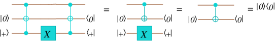
Figure 2: How to simulate measurement of $|0\rangle\langle 0|$ by measurement of $X$.

If $k=1$ one can choose $W\,|\psi\rangle=T[1,3;2]\,|\psi\rangle\otimes|0\rangle\otimes|+\rangle$, where $T[1,3;2]$ is the Toffoli gates with control qubits $1,3$ and target qubit $2$, that is

$$T[1,3;2]\,|a,b,c\rangle=|a,b\oplus ac,c\rangle.$$

One can easily check that

$$T[1,3;2]\,(I\otimes I\otimes X)\,T[1,3;2]^{\dagger}=\mbox{CNOT}[1;2]\otimes X.$$

Accordingly, $W^{\dagger}\,(I\otimes I\otimes X)\,W=\langle 0_{2}|\,\mbox{CNOT}[1;2]\,|0_{2}\rangle\langle+|X|+\rangle=|0\rangle\langle 0|$, see Figure 2. For arbitrary $k$ one can use $k$ copies of the ancilla $|0\rangle$ and $k$ Toffoli gates, i.e., $W\,|\psi\rangle=\prod_{j=1}^{k}T[j,2k+1;j+k]\,|\psi\rangle\otimes|0\rangle^{\otimes k}\otimes|+\rangle$ (all Toffoli gates in the product commute). The proof of Eq. (12) is the same except for not using the ancilla $|+\rangle$, i.e., $W\,|\psi\rangle=\prod_{j=1}^{k-1}T[j,2k-1;j+k-1]\,|\psi\rangle\otimes|0\rangle^{\otimes k-1}$. ∎

References

- [1] S. Bravyi, D. DiVincenzo, R. Oliveira, and B. Terhal. The Complexity of Stoquastic Local Hamiltonian Problems. http://arxiv.org/abs/quant-ph/0606140.
- [2] L. Babai. Trading group theory for randomness. In Proceedings of 17th STOC, pages 421–429, 1985.
- [3] S. Bravyi. Efficient algorithm for a quantum analogue of 2-SAT. http://arxiv.org/abs/quant-ph/0602108.
- [4] C. H. Papadimitriou. Computational Complexity. 1994, Addison-Wesley.
- [5] S. Goldwasser and M Sipser, Private coins versus public coins in interactive proof systems In STOC ’86: Proceedings of the eighteenth annual ACM symposium on Theory of computing, pages 59–68, 1986. DOI http://doi.acm.org/10.1145/12130.12137
- [6] A. Kitaev, A. Shen, and M. Vyalyi. Classical and Quantum Computation. Vol. 47 of Graduate Studies in Mathematics. American Mathematical Society, Providence, RI, 2002.
- [7] J. Watrous. Succinct quantum proofs for properties of finite groups. Proceedings of 41st FOCS, p. 537, 2000.
- [8] D. Aharonov and T. Naveh. Quantum NP - A Survey. http://arxiv.org/abs/quant-ph/0210077.
- [9] D. Aharonov and O. Regev. A Lattice Problem in Quantum NP. http://arxiv.org/abs/quant-ph/0307220.
- [10] J. Kempe, A. Kitaev, and O. Regev. The Complexity of the Local Hamiltonian Problem. SIAM Journal of Computing, 35, p. 1070, 2006.
- [11] D. Janzing, P. Wocjan, and T. Beth. Identity check is QMA-complete. http://arxiv.org/abs/quant-ph/0305050.
- [12] R. Oliveira and B. Terhal. The complexity of quantum spin systems on a two-dimensional square lattice. http://arxiv.org/abs/quant-ph/0504050.
- [13] S. Aaronson and G. Kuperberg. Quantum versus classical proofs and advice. http://arxiv.org/abs/quant-ph/0604056.
- [14] Y. Liu. Consistency of Local Density Matrices is QMA-complete. http://arxiv.org/abs/quant-ph/0604166.
- [15] Y. Liu, M. Christandl, and F. Verstraete. N-representability is QMA-complete. http://arxiv.org/abs/quant-ph/0609125.
- [16] O. Goldreich, S. Micali and A. Wigderson, “Proofs that yield nothing but their validity”, Proceedings of FOCS 86, pp. 174–187.
- [17] E. Böhler, C. Glaßer, and D. Meister. Error-bounded probabilistic computations between MA and AM. In Proceedings of 28th MFCS, pages 249-258, 2003.
- [18] Y. Han, L. Hemaspaandra, and T. Thierauf. Threshold computation and cryptographic security. SIAM Journal of Computing, 26(1), pages 59–78, 1997.
- [19] M. Furer, O. Goldreich, Y. Mansour, M. Sipser, and S. Zachos. On completeness and soundness in Interactive Proof Systems. Advances in Computing Research, 5, pages 429–442, 1989.
- [20] D. Aharonov, W. van Dam, Z. Landau, S. Lloyd, J. Kempe, and O. Regev. Universality of Adiabatic Quantum Computation. In Proceedings of 45th FOCS, 2004, http://arxiv.org/abs/quant-ph/0405098.
- [21] V. Arvind , J. Kobler, U. Schoning and R. Schuler If NP Has Polynomial-Size Circuits then MA=AM Theoretical Computer Science 137, pages 279-282 (1995).