Single observable concurrence measurement without simultaneous copies

Abstract

We present a protocol that allows us to obtain the concurrence of any two qubit pure state by performing a minimal and optimal tomography of one of the subsystems through measuring a single observable of an ancillary four dimensional qudit. An implementation for a system of trapped ions is also proposed, which can be achieved with present day experimental techniques.

Even if entanglement was spotted as a key feature of quantum mechanics since the early days of the theory schrodinger , it was only with the advent of quantum information science that a great deal of attention was drawn upon the problems of characterizing, properly quantifying, and ultimately measuring entanglement bennett:247 .

Until recently, measurements of entanglement had only been achieved indirectly by performing measurements on several non-commuting observables of the system, and then adequately combining the results james:052312 . A direct measurement of concurrence (previously shown to be a proper entanglement measure wootters:2245 ), however, was reported in walborn06 , in which two copies of the state were used simultaneously, following the idea in florian . Although this experiment constitutes a landmark on the path towards fully understanding quantum entanglement, a simpler measurement, which does not involve simultaneous copies, is desirable.

In the simplest case where we deal with a pure state of two qubits, one way to address the problem is to take advantage of a well-known relation between the bipartite concurrence and the reduced density matrix of either subsystem coffman:052306 :

$$C^{2}=4\det\rho_{q},$$ (1)

where $\rho_{q}$ is the reduced density matrix of one of the qubits and $C$ is the bipartite concurrence. Hence, the concurrence of the system can be obtained by performing the tomography of only one of the qubits.

In ref. rehacek:052321 , Řeháček et al. presented a protocol for optimal minimal qubit tomography, in which all information pertaining to the state of one qubit is obtained by measuring the population of the states of two ancillary qubits, which are previously entangled with the target qubit by nonlocal operations. In a loose sense, information of the measured qubit is “written” in the ancillas: the three values $\langle\hat{\sigma}_{x}\rangle$, $\langle\hat{\sigma}_{y}\rangle$ and $\langle\hat{\sigma}_{z}\rangle$ necessary for qubit tomography are encoded into the four probabilities $P_{jk}$ $(j,k=0,1)$ of the ancillary system to be found in each state $|jk\rangle$, of which only three are independent because of the unity sum requirement. An implementation where the qubit was encoded in linear photon polarizations and different paths in an optical interferometer played the role of ancillary qubits was also proposed. Later on, this proposal was experimentally achieved ling:022309 .

The aim of this article is twofold: first, we want to point out the fact that concurrence for a two qubit pure state can be obtained through measurement of the probability distribution of the spectrum of a single observable, without the need of simultaneous copies of the state. This is achieved by performing a minimal and optimal tomography of one of the qubits via a single measurement on an ancillary four dimensional system. The tomography is minimal in the sense that no redundant information is obtained from the measurements (as opposed to the standard procedure) and optimal in that it achieves maximum accuracy in determining an unknown state rehacek:052321 . Even if the procedure developed in rehacek:052321 could in principle be used for such an end, we will use in order to illustrate our point a tomographic protocol of our own, in which the fact that the probability distribution of the spectrum of a single observable is being measured appears naturally. By introducing a four level qudit as our ancillary system, we are able to “write” the three desired values in the populations of the four levels of the ancilla $P_{G}$, $P_{G^{\prime}}$, $P_{E}$ and $P_{E^{\prime}}$, of which only three are independent. By choosing these states to have different energies, we can pick the observable to be the energy of the ancilla.

Second, we propose an implementation of the protocol for a system of trapped ions, which is achievable with present day experimental techniques. Our protocol proves simpler to implement for this kind of systems than that in rehacek:052321 , for it uses one less ancilla, which means that one less ion is involved.

In what follows, we will denote by $|\chi\rangle$ the two qubit pure state on which tomography of one qubit is to be performed, and $|G\rangle$, $|G^{\prime}\rangle$, $|E\rangle$ and $|E^{\prime}\rangle$ the four distinct states of the ancilla. We will make use of two kinds of operations:

i) Rotations between ancillary states. These are denoted by $\hat{R}_{\alpha}^{JK}(\theta)=\exp\left(-i\frac{\theta}{2}\hat{\sigma}_{\alpha}^{JK}\right)$, where $\hat{\sigma}_{\alpha}^{JK}$ is one of the Pauli operators ($\alpha\in\{x,y,z\}$) defined on the subspace spanned by the arbitrary states $|J\rangle$ and $|K\rangle$:

$$\begin{split}\hat{\sigma}_{x}^{JK}&=|K\rangle\langle J|+|J\rangle\langle K|\\ \hat{\sigma}_{y}^{JK}&=-i(|K\rangle\langle J|-|J\rangle\langle K|)\\ \hat{\sigma}_{z}^{JK}&=|K\rangle\langle K|-|J\rangle\langle J|.\\ \end{split}$$ (2)

ii) Controlled operations applied on the target qubit and controlled by the ancilla. These are denoted by $C^{A}\hat{U}$, where $A\in\{G,G^{\prime},E,E^{\prime}\}$ denotes the control ancillary state whose occupation implies action of operator $\hat{U}$ on the selected qubit. We can have, for instance: $C^{E}\hat{U}\frac{1}{\sqrt{2}}\left(|G\rangle+|E\rangle\right)|\chi\rangle=\frac{1}{\sqrt{2}}\left(|G\rangle+|E\rangle\hat{U}\right)|\chi\rangle$, where we explicitly put operator $\hat{U}$, which acts only on the target qubit, to the right of the ancilla ket. Only three instances of $\hat{U}$ will be actually realized: $\hat{\sigma}_{x}$, $\hat{\sigma}_{y}$ and $-\hat{\sigma}_{z}$, which are unitary operations on the qubit, whose basis states are denoted by $|g_{q}\rangle$ and $|e_{q}\rangle$.

Protocol. Our protocol starts with the system in the state $|G\rangle|\chi\rangle.$ To this initial state, we apply three successive rotations, $R_{y}^{GE}(\theta_{1})$, $R_{y}^{GG^{\prime}}(\theta_{2})$ and $R_{y}^{G^{\prime}E^{\prime}}(\theta_{3})$ with $\theta_{1}$, $\theta_{2}$ and $\theta_{3}$ such that

$$\begin{split}R_{y}^{GE}(\theta_{1})|G\rangle&=\frac{1}{\sqrt{6}}\left(\sqrt{5}|G\rangle+|E\rangle\right),\\ R_{y}^{GG^{\prime}}(\theta_{2})|G\rangle&=\frac{1}{\sqrt{5}}\left(\sqrt{3}|G\rangle+\sqrt{2}|G^{\prime}\rangle\right),\\ R_{y}^{G^{\prime}E^{\prime}}(\theta_{3})|G^{\prime}\rangle&=\frac{1}{\sqrt{2}}\left(|G^{\prime}\rangle-|E^{\prime}\rangle\right).\end{split}$$ (3)

We thus obtain the state

$$\frac{1}{\sqrt{2}}\left(|G\rangle+\frac{1}{\sqrt{3}}|G^{\prime}\rangle+\frac{1}{\sqrt{3}}|E\rangle-\frac{1}{\sqrt{3}}|E^{\prime}\rangle\right)|\chi\rangle.$$ (4)

The next step of the protocol requires us to perform the controlled operations $C^{G^{\prime}}(\hat{\sigma}_{y})$, $C^{E}(\hat{\sigma}_{x})$ and $C^{E^{\prime}}(-\hat{\sigma}_{z})$, ending up with the following state:

$$\frac{1}{\sqrt{2}}\left(|G\rangle+\frac{1}{\sqrt{3}}|G^{\prime}\rangle\hat{\sigma}_{y}+\frac{1}{\sqrt{3}}|E\rangle\hat{\sigma}_{x}+\frac{1}{\sqrt{3}}|E^{\prime}\rangle\hat{\sigma}_{z}\right)|\chi\rangle.$$ (5)

Finally we apply the following local $\pi/2$ rotations around the $y$ axis on the ancilla: $\hat{R}_{y}^{GE}\left(\frac{\pi}{2}\right)$, $\hat{R}_{y}^{G^{\prime}E^{\prime}}\left(\frac{\pi}{2}\right)$, $\hat{R}_{y}^{GG^{\prime}}\left(\frac{\pi}{2}\right)$ and $\hat{R}_{y}^{EE^{\prime}}\left(\frac{\pi}{2}\right)$ to obtain:

$$\left(|G\rangle\hat{Q}_{G}-|G^{\prime}\rangle\hat{Q}_{G^{\prime}}-|E\rangle\hat{Q}_{E}+|E^{\prime}\rangle\hat{Q}_{E^{\prime}}\right)|\chi\rangle,$$ (6)

where we have:

$$\begin{split}\hat{Q}_{G}&=\frac{1}{2\sqrt{2}}\left(\hat{\openone}+\frac{1}{\sqrt{3}}\left(\hat{\sigma}_{x}+\hat{\sigma}_{y}+\hat{\sigma}_{z}\right)\right),\\ \hat{Q}_{G^{\prime}}&=\frac{1}{2\sqrt{2}}\left(\hat{\openone}+\frac{1}{\sqrt{3}}\left(\hat{\sigma}_{x}-\hat{\sigma}_{y}-\hat{\sigma}_{z}\right)\right),\\ \hat{Q}_{E}&=\frac{1}{2\sqrt{2}}\left(\hat{\openone}+\frac{1}{\sqrt{3}}\left(-\hat{\sigma}_{x}+\hat{\sigma}_{y}-\hat{\sigma}_{z}\right)\right),\\ \hat{Q}_{E^{\prime}}&=\frac{1}{2\sqrt{2}}\left(\hat{\openone}+\frac{1}{\sqrt{3}}\left(-\hat{\sigma}_{x}-\hat{\sigma}_{y}+\hat{\sigma}_{z}\right)\right).\end{split}$$ (7)

We then readily calculate the probabilities for the ancilla to be found in each state:

$$\begin{split}P_{G}&=\frac{1}{4}\left(1+\frac{1}{\sqrt{3}}(\langle\hat{\sigma}_{x}\rangle+\langle\hat{\sigma}_{y}\rangle+\langle\hat{\sigma}_{z}\rangle)\right)\\ P_{G^{\prime}}&=\frac{1}{4}\left(1+\frac{1}{\sqrt{3}}(\langle\hat{\sigma}_{x}\rangle-\langle\hat{\sigma}_{y}\rangle-\langle\hat{\sigma}_{z}\rangle)\right)\\ P_{E}&=\frac{1}{4}\left(1+\frac{1}{\sqrt{3}}(-\langle\hat{\sigma}_{x}\rangle+\langle\hat{\sigma}_{y}\rangle-\langle\hat{\sigma}_{z}\rangle)\right)\\ P_{E^{\prime}}&=\frac{1}{4}\left(1+\frac{1}{\sqrt{3}}(-\langle\hat{\sigma}_{x}\rangle-\langle\hat{\sigma}_{y}\rangle+\langle\hat{\sigma}_{z}\rangle)\right).\end{split}$$ (8)

By adding and subtracting these probabilities, we can obtain any mean value $\langle\hat{\sigma}_{\alpha}\rangle$, which means we have successfully performed the tomography of the qubit just by measuring the populations of the energy eigenstates of the ancilla.

We would like to stress that the four values of the probabilities in Eq. 8 are the expectation values of the operators $\hat{Q}_{G}^{2},$ $\hat{Q}_{G^{\prime}}^{2},$ $\hat{Q}_{E}^{2}$ and $\hat{Q}_{E^{\prime}}^{2}$, which constitute a minimal and optimal POVM rehacek:052321 for the one qubit tomography we are considering.

Having performed the tomography of one of the qubits, it is straightforward to find the value of the concurrence of the bipartite system using relation (1). In terms of the occupation probabilities, it is given by:

$$C^{2}=4\left(1-3(P_{G}^{2}+P_{G^{\prime}}^{2}+P_{E}^{2}+P_{E^{\prime}}^{2})\right)$$ (9)

We thus managed to obtain the value of the concurrence by measuring the probability distribution of the spectrum of a single observable of a four dimensional ancillary system, with no need of simultaneous copies of the state. We stress the fact that even if only the expectation value of an observable is needed instead of the complete probability distribution in schemes using simultaneous copies, in practice this distribution must be determined anyway in order to compute the expectation value walborn06 .

Trapped Ions Implementation. Consider now a system of ions inside a linear Paul trap. To a good approximation, the effect of the trap in the motion of the ions can be described by a harmonic oscillator. The qubits are encoded in ground and excited electronic states of each ion, while one of the ions plays the role of the ancillary system. When an ion is illuminated by laser light quasi-resonant with one of its electronic transitions, the collective motional degrees of freedom can be coupled to the electronic ones via photon-momentum exchange. The laser excitation can be done in several different ways, giving rise to a large number of possible interaction Hamiltonians. Here we will be interested in a situation where the motional sidebands are well resolved and the so-called Lamb–Dicke limit applies. Moreover, we will only consider the excitation of one collective motional degree of freedom, the center of mass (CM) motional mode in the longitudinal trap direction.

In order to perform the operations requested by the protocol, we have to consider the laser excitation of any given electronic transition of an ion in three different ways. One consists in illuminating the ion with laser light resonant with the transition, often called carrier excitation. The second way is to excite the transition with light resonant with the first lower motional sideband (red sideband); and the last one uses light resonant with the first higher sideband (blue sideband).

Under the conditions stated above, the interaction Hamiltonians corresponding to each one of these situations are given, in the interaction picture, by vogel:4214 :

$$\hat{H}_{\rm C} = \frac{1}{2}\hbar\,|\Omega|\,e^{i\phi}\,\hat{\sigma}_{+}+\mbox{h.c.}$$ (10)

$$\hat{H}_{\rm R} = \frac{i}{2}\eta\hbar\,|\Omega|\,e^{i\phi}\,\hat{\sigma}_{+}\,\hat{a}+\mbox{h.c.}$$ (11)

$$\hat{H}_{\rm B} = \frac{i}{2}\eta\hbar\,|\Omega|\,e^{i\phi}\,\hat{\sigma}_{+}\,\hat{a}^{\dagger}+\mbox{h.c.},$$ (12)

respectively. Here the operator $\hat{\sigma}_{+}$ is the electronic raising operator, and $\hat{a}$ and $\hat{a}^{\dagger}$ are the annihilation and creation operators of the CM vibrational mode, respectively. $\Omega=|\Omega|e^{i\phi}$ is the laser Rabi frequency and $\eta$ is the Lamb–Dicke parameter, which in the Lamb–Dicke limit satisfies $\eta\ll 1$.

The rotations appearing in the protocol are performed via carrier excitation of the ions, according to the time evolution operator:

$$e^{-\frac{i}{\hbar}\hat{H}_{\rm C}\tau}=\hat{U}_{\rm C}(\theta,\phi)=e^{-i\frac{\theta}{2}\left(\cos(\phi)\,\hat{\sigma}^{ge}_{x}-\sin(\phi)\,\hat{\sigma}^{ge}_{y}\right)}\;,$$ (13)

where $\theta=|\Omega|\tau$ and $\hat{\sigma}^{ge}_{\alpha}$ are the electronic Pauli operators (see Eq. (2)), acting on the subspace spanned by $|g\rangle$ and $|e\rangle$, these in turn representing generic ground ($|G\rangle$, $|G^{\prime}\rangle$, $|g_{q}\rangle$) and excited ($|E\rangle$, $|E^{\prime}\rangle$, $|e_{q}\rangle$) states, respectively. In particular, the rotations $\hat{R}^{ge}_{x}(\theta)=\hat{U}_{\rm C}(\theta,0)$ and $\hat{R}^{ge}_{y}(\theta)=\hat{U}_{\rm C}(\theta,-\pi/2)$ are obtained by adjusting the laser phase.

Controlled operations are achieved through excitation of the CM vibrational mode. Both Jaynes–Cummings (red sideband, Eq. (11)) and anti Jaynes–Cummings (blue sideband, Eq. (12)) interactions are used in the protocol.

For concreteness, we present an implementation using ${}^{40}{\rm Ca}^{+}$ ions, which have been used in several experiments in Innsbruck riebe:734 . States $|g_{q}\rangle$ and $|e_{q}\rangle$ of each qubit can be encoded in sublevels $m=-1/2$ of the $4S_{1/2}$ state and $m=-1/2$ of the $3D_{5/2}$ state, respectively.

We further use another ${}^{40}{\rm Ca}^{+}$ ion for our four level ancilla. States $|G\rangle$ and $|G^{\prime}\rangle$ can be associated to the $m=-1/2$ and the $m=1/2$ sublevels of the $4S_{1/2}$ state, respectively, while states $|E\rangle$ and $|E^{\prime}\rangle$ can be associated to the $m=3/2$ and $m=-3/2$ sublevels of the metastable $3D_{3/2}$ state (see fig. 1).

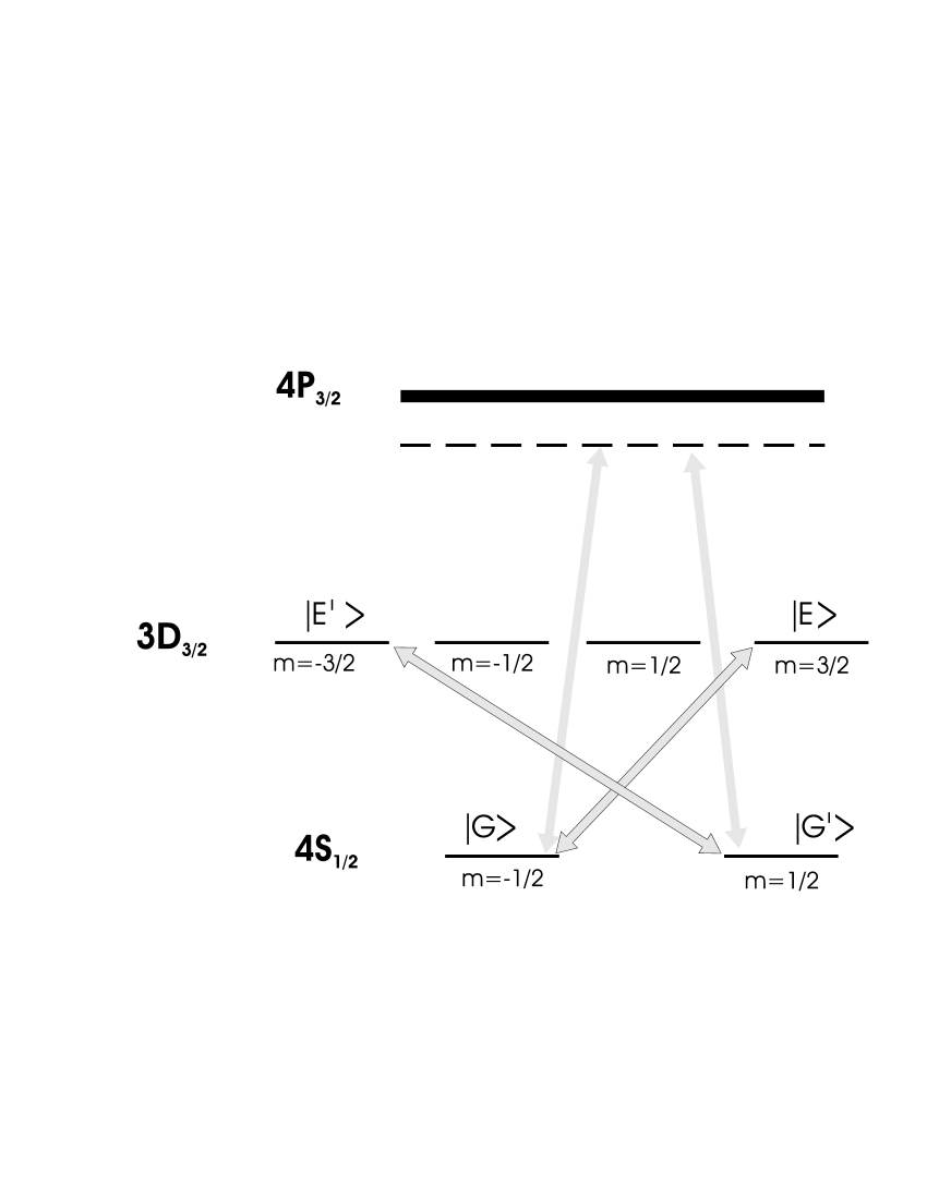
Figure 1: Encoding of the ancillary ion and relevant transitions

The first part of the protocol consists in preparing the ancilla in the superposition given by Eq. (4). Since $4S_{1/2}\leftrightarrow 3D_{3/2}$ is a quadrupole transition, it is possible to select sublevel transitions with $\Delta m=\pm 2$ by controlling the angle between the incident laser beam and the direction of a weak applied magnetic field, as well as the laser polarization. These transitions allow us to perform rotations between specific ground and excited levels without disturbing the rest. Rotations $R_{y}$ among the two ground state levels $|G\rangle$ and $|G^{\prime}\rangle$ are performed through a carrier Raman excitation, which can be achieved through simultaneous off-resonant excitation of the dipole transition $4S_{1/2}\leftrightarrow 4P_{3/2}$ by two laser beams of polarizations $\pi$ and $\sigma_{+}$ focused on the ancillary ion.

We start with the system in state $|G\rangle|\chi\rangle|0\rangle_{v}$, where $|0\rangle_{v}$ is the ground state of the CM vibrational mode. In order to perform the first rotation $R_{y}^{GE}(\theta_{1})$ we apply a carrier excitation of the $4S_{1/2}\leftrightarrow 3D_{3/2}$ quadrupole transition with $\Delta m=2$. This rotation is followed by a carrier Raman excitation among levels $|G\rangle$ and $|G^{\prime}\rangle$ as described above, implementing $R_{y}^{GG^{\prime}}(\theta_{2})$. We finally perform the $R_{y}^{G^{\prime}E^{\prime}}(\theta_{3})$ rotation applying a carrier excitation of the $4S_{1/2}\leftrightarrow 3D_{3/2}$ transition with $\Delta m=-2$. After that series of laser pulses, the electronic state of the ions is given by Eq. (4), with the vibrational CM mode still unoccupied.

Next in the protocol are the controlled operations. First, we want to apply $\hat{\sigma}_{y}$ on $|\chi\rangle$ controlled by state $|G^{\prime}\rangle$. We apply on the ancilla a $\pi$-pulse resonant with the first blue sideband of the $4S_{1/2}\leftrightarrow 3D_{3/2}$ transition with $\Delta m=-2$, and with phase $\phi=0$. (This choice of phase will be maintained for all red and blue detuned pulses). This anti Jaynes–Cummings interaction takes state $|G^{\prime}\rangle|\chi\rangle|0\rangle_{v}$ to $|E^{\prime}\rangle|\chi\rangle|1\rangle_{v}$, leaving the other states unchanged. With this operation we transfer the information about the occupation of state $|G^{\prime}\rangle$ to the motional state $|1\rangle_{v}$. We now apply $\hat{\sigma}_{y}$ on the qubit, controlled by the motional state $|1\rangle_{v}$. We achieve this by performing a carrier rotation $R^{g_{q}e_{q}}_{x}(-\pi/2)$ on the qubit, followed by a $2\pi$-pulse resonant with the first red sideband of the transition between level $|g_{q}\rangle$ and an auxiliary level $|e^{\prime}_{q}\rangle$, which takes $|g_{q}\rangle|\chi\rangle|1\rangle_{v}$ back to itself through $|e^{\prime}_{q}\rangle|\chi\rangle|0\rangle_{v}$, while gaining a minus sign. We then apply a carrier rotation $R^{g_{q}e_{q}}_{x}(\pi/2)$ on the qubit to obtain state $-|E^{\prime}\rangle\hat{\sigma}_{y}|\chi\rangle|1\rangle_{v}$. Finally, another $\pi$-pulse on the ancilla resonant with the first blue sideband of the $4S_{1/2}\leftrightarrow 3D_{3/2}$ transition will bring the state $-|E^{\prime}\rangle\hat{\sigma}_{y}|\chi\rangle|1\rangle_{v}$ to $|G^{\prime}\rangle\hat{\sigma}_{y}|\chi\rangle|0\rangle_{v}$. Notice that all other states remain unaffected by these transformations.

An analogous procedure is followed in order to act on the qubit with $\hat{\sigma}_{x}$, controlled by state $|E\rangle$: we first apply on the ancilla a $\pi$-pulse resonant with the first red sideband of the $4S_{1/2}\leftrightarrow 3D_{3/2}$ transition with $\Delta m=2$, which transforms state $|E\rangle|\chi\rangle|0\rangle_{v}$ into $-|G\rangle|\chi\rangle|1\rangle_{v}$. Then we apply on the target ion a $R^{g_{q}e_{q}}_{y}(\pi/2)$ rotation, followed by a $2\pi$-pulse resonant with the first red sideband of the $|g_{q}\rangle\leftrightarrow|e^{\prime}_{q}\rangle$ transition, and a $R^{g_{q}e_{q}}_{y}(-\pi/2)$ rotation. Finally, we apply on the ancilla another red sideband $\pi$-pulse, identical to the first one.

The $-\hat{\sigma}_{z}$ operation, controlled by level $|E^{\prime}\rangle$ can be achieved by applying the following sequence of pulses: a $\pi$-pulse with $\Delta m=-2$ resonant with the first red sideband of the $4S_{1/2}\leftrightarrow 3D_{3/2}$ transition on the ancilla, a $2\pi$-pulse resonant with the first red sideband of the $|g_{q}\rangle\leftrightarrow|e^{\prime}_{q}\rangle$ transition on the target ion, and another $\pi$-pulse on the ancilla, identical to the first. After these three controlled operations are performed, the system is left in the state given by equation (5), with no excitations in the vibrational mode.

We complete the protocol by performing the four rotations: $\hat{R}_{y}^{GE}\left(\frac{\pi}{2}\right)$, $\hat{R}_{y}^{G^{\prime}E^{\prime}}\left(\frac{\pi}{2}\right)$, $\hat{R}_{y}^{GG^{\prime}}\left(\frac{\pi}{2}\right)$ and $\hat{R}_{y}^{EE^{\prime}}\left(\frac{\pi}{2}\right)$, by applying successive carrier laser pulses. We obtain thus the state given by Eq. (6).

At this point, we need to measure the populations of the ancillary electronic states. This is accomplished, via electronic shelving technique, by exciting the $4S_{1/2}\leftrightarrow 4P_{1/2}$ transition and monitoring the fluorescence light leibfried:281 . In our case, a preliminary series of laser pulses is needed in order to prepare the ancillary ion for measurement.

First, a carrier Raman $\pi$-pulse excites the $3D_{3/2}\leftrightarrow 3D_{5/2}$ transition via the $4P_{3/2}$ level, using two $\pi$-polarized laser beams. This brings the population of state $|E\rangle$ to the Zeeman sublevel $3D_{5/2}$ $(m=3/2)$ and the population of $|E^{\prime}\rangle$ to $3D_{5/2}$ $(m=-3/2)$. Then, a $\pi$-pulse with $\Delta m=2$ resonant with the $4S_{1/2}\leftrightarrow 3D_{3/2}$ transition is applied, bringing the population of state $|G\rangle$ to $3D_{3/2}$ $(m=3/2)$, followed by a $\pi$-pulse with $\Delta m=0$ resonant with the $4S_{1/2}\leftrightarrow 3D_{5/2}$ transition, bringing the population of state $|G^{\prime}\rangle$ to $3D_{5/2}$ $(m=1/2)$. Finally, a $\pi$-pulse with $\Delta m=2$ resonant with the $4S_{1/2}\leftrightarrow 3D_{3/2}$ transition is applied, bringing the population of state $|G\rangle$ back to level $4S_{1/2}$ $(m=-1/2)$.

Now transition $4S_{1/2}\leftrightarrow 4P_{1/2}$ is excited and fluorescence light is monitored. If fluorescence is observed, this indicates that the ancillary state $|G\rangle$ was occupied, and the measurement ends. Otherwise, a $\pi$-pulse with $\Delta m=0$ resonant with the $4S_{1/2}\leftrightarrow 3D_{5/2}$ transition is applied, bringing the population of state $|G^{\prime}\rangle$ back to level $4S_{1/2}$ $(m=1/2)$. The fluorescence test is repeated, a positive result indicating that state $|G^{\prime}\rangle$ was occupied. Again, if no fluorescence is observed, a $\pi$-pulse with $\Delta m=2$ resonant with the $4S_{1/2}\leftrightarrow 3D_{5/2}$ transition is applied, bringing the population of state $|E\rangle$ to $4S_{1/2}$ $(m=-1/2)$. The fluorescence test is repeated once more, now a positive result indicating occupation of the $|E\rangle$ state. No light observed in this last test indicates that state $|E^{\prime}\rangle$ was the one occupied. Several iterations of this process yield the occupation probabilities of the four ancillary levels. This whole procedure is equivalent to measuring the probability distribution of the spectrum of a single observable: the electronic energy of the ancilla.

We wish to note that the whole series of pulses would be considerably reduced by taking advantage of the Zeeman splitting of the levels obtained with a strong applied magnetic field, but this would also limit the initial Doppler cooling of the ions thesis .

We would like to stress that our protocol is designed for pure states. However, if we consider small deviations from a pure state we still may have a good estimate for the concurrence. Assuming, for example, a density matrix of the form $\rho=\lambda\rho^{\prime}+(1-\lambda)|\chi\rangle\langle\chi|$, where $\rho^{\prime}$, is a separable state and $\lambda\ll 1$, then one can show that the difference between the values of the square of the true concurrence and the value obtained using the above protocol is $-2\lambda(1-\vec{P}\cdot\vec{P^{\prime}})+{\cal O}(\lambda^{2})$, where $\vec{P^{\prime}}$ and $\vec{P}$ are the Bloch vectors associated with the reduced density matrices of $\rho^{\prime}$ and $|\chi\rangle\langle\chi|$, respectively.

Before concluding we would like to briefly compare our protocol with measurements involving simultaneous copies florian ; walborn06 . Clearly, the main difference lies in the fact that we do not require simultaneous copies of the state in order to measure concurrence. Another advantage of our protocol is that, given that the relation stated in Eq. (1) holds for the bipartite concurrence of a qubit with an arbitrary number of other qubits, provided they are all in a pure state, our protocol is trivially generalized to this case. It is also important to note that we do not have an extra cost for not using simultaneous copies: the four dimensions of our ancilla match those in the two qubits where the copy of the system is provided.

As compared to standard tomography, our protocol not only involves a single observable, but is also minimal and optimal, implying in particular that improved accuracy is achieved in determining the state of the system.

In summary, we presented a minimal and optimal tomographic protocol which involves the measurement of a single observable. This in turn is used to obtain the concurrence of a pure two qubit state. We also propose a realistic implementation of the protocol for a system of trapped ions, which could in principle be carried out with present day experimental techniques.

- (1) E. Schrödinger, Naturwissenschaften 23, 807 (1935), A. Einstein, B. Podolsky, and N. Rosen, Phys. Rev. 47, 777 (1935).
- (2) C. Bennett and D. P. DiVincenzo, Nature 404, 247 (2000).
- (3) D. F. V. James et al., Phys. Rev. A 64, 052312 (2001). C. F. Roos et al., Phys. Rev. Lett. 92, 220402 (2004).
- (4) W. K. Wootters, Phys. Rev. Lett. 80, 2245 (1998).
- (5) S. P. Walborn et al., Nature 440, 10022 (2006).
- (6) F. Mintert et al., Phy. Rep. 415, 207 (2005).
- (7) V. Coffman, J. Kundu, and W. K. Wootters, Phys. Rev. A 61, 052306 (2000).
- (8) J. Rehacek, B.-G. Englert, and D. Kaszlikowski, Phys. Rev. A70, 052321 (2004).
- (9) A. Ling et al., Physical Review A (Atomic, Molecular, and Optical Physics) 74, 022309 (2006).
- (10) M. Nielsen and I. L. Chuang, Quantum Information and Quantum Computation (Cambridge University Press, 2000).
- (11) W. Vogel and R. L. de Matos Filho, Phys. Rev. A 52, 4214 (1995).
- (12) See for example M. Riebe et al., Nature 429, 734 (2004).
- (13) D. Leibfried et al., Rev. Mod. Phys. 75, 281 (2003).
- (14) Andreas B. Mundt, PhD. Thesis, Universität Innsbruck (2003).