Quantum entanglement of two flux qubits induced by an auxiliary SQUID

Abstract

We revisit a theoretical scheme to create quantum entanglement of two three-levels superconducting quantum interference devices (SQUIDs) with the help of an auxiliary SQUID. In this scenario, two three-levels systems are coupled to a quantized cavity field and a classical external field and thus form dark states. The quantum entanglement can be produced by a quantum measurement on the auxiliary SQUID. Our investigation emphasizes the quantum effect of the auxiliary SQUID. For the experimental feasibility and accessibility of the scheme, we calculate the time evolution of the whole system including the auxiliary SQUID. To ensure the efficiency of generating quantum entanglement, relations between the measurement time and dominate parameters of the system are analyzed according to detailed calculations.

Key words: superconducting quantum interference device, entangled state, quantum information, dark state

I I. Introduction

Recently, superconducting quantum circuits (SQCs) based on superconducting quantum interference devices (SQUIDs) Makhlin ; Nakamura ; Rouse ; Han ; Chu , have appeared to be among the most promising candidates for quantum information processing. Especially, schemes of quantum information transfer (QIT) and quantum entanglement by using SQC in a microwave cavity are carried out in many experiments Yang ; Steinbach ; Yu ; Berkley . The essential idea beyond these schemes is listed as follows. Firstly, one should make several SQUIDs Shnirman coupling to a single mode quantum field in a microwave cavity. Secondly, QIT in the quantum computing can be realized by adjusting the external field to carry out a sequence of quantum logic operations on SQUIDs.

In this aspect, there are many experiments by using SQUIDs Yang ; Steinbach to realize quantum entanglement of macroscopic quantum devices. Here, a theoretical protocol has been proposed based on the experimentally accessible parameters SI ; Yang ; Zhou ; ZE , in which two SQUIDs are placed into a microwave cavity. Each flux qubit has a $\Lambda$-type energy level configuration. An external classical field is applied to this system. Because these two three-level artificial atoms (or SQUIDs) couple to a single-mode quantum field simultaneously, an effective coupling between two three-level systems are induced by this single mode field. This field behaves as a data bus to link two qubits coherently. When two three-level systems coupling to two fields, a classical field and a quantized cavity mode, there is usually a dark state, which contains a component with maximal entanglement of two qubits. To realize the maximal quantum entanglement between two qubits via the dark state, an auxiliary SQUID is used to carry out a projective quantum measurement. As a result of post selection measurement by wave function collapse, a quantum state with maximal entanglement can be obtained.

Although this scheme is very subtle in the theoretical setup, there are still some further considerations of physical mechanism needed. Especially, the influence of the auxiliary SQUID should be taken into account since it should be treated as a quantum subsystem. According to the contemporary theory of quantum measurement, apparatus are usually considered as a quantum subsystem interacting with the measured system. In fact, the quantum effect of an auxiliary SQUID in Kansas scheme Yang is not considered in details. In this paper, we will stress the quantum effect of the auxiliary SQUID with respect to the whole quantum system. Our result shows that the back action of the auxiliary SQUID on two qubits cannot be ignored.

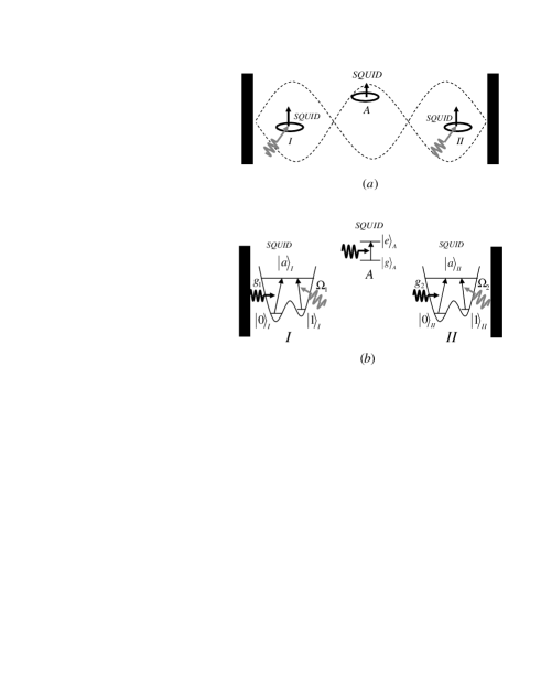
Figure 1: Schematic illustration of the setup. (a) Two SQUIDs and a auxiliary SQUID are put in a microwave cavity. Here, the black line (dashed lines) denotes single mode cavity quantum field and grey lines denote microwave classical fields. (b) Black lines denote single mode cavity quantum fields. Grey lines denote microwave classical fields. Coupling constants between the cavity field and two SQUIDs are $g_{l}$ ($l=1,2$). Coupling constants between the external microwave field and two SQUIDs are $\Omega_{l}$ ($l=1,2$).

II II. The General description of quantum entanglement scheme of SQUIDs

This paper is based on the theoretical proposal of Ref. Yang . We first briefly review the essential idea of this paper with the setup being illustrated in Fig. 1. In each SQUID ($I$ and $II$) the transition from the ground state $\left|0\right\rangle_{l}$ to the excited state $\left|a\right\rangle_{l}$ resonates with the same single-mode cavity field. The transition from the first excited state $\left|1\right\rangle_{l}$ to the excited state $\left|a\right\rangle_{l}$ resonates with a external classical field. The Hamiltonian $H_{0}$ Yang ; You ; Nori is written in the interaction picture as

$$H_{0}=\sum_{l=I,II}(g_{l}c\left|a\right\rangle_{l}\left\langle 0\right|+\Omega_{l}\left|a\right\rangle_{l}\left\langle 1\right|+H.c.)\text{,}$$ (1)

where $g_{l}$ $\left(l=I,II\right)$ are coupling constants between the cavity field and two SQUIDs respectively, $\Omega_{l}$ $\left(l=I,II\right)$ are coupling constants between the external field and the two SQUIDs respectively, $c^{\dagger}$ and $c$ are creation and annihilation operators of the cavity field mode. In Ref. Yang , $\Omega_{l}$ is time dependent to investigate the dynamics of a quantum information transfer between two SQUIDs. In this paper we only concern the quantum entanglement of SQUIDs and the effect of the auxiliary SQUID. So $\Omega_{l}$ is a constant throught this paper.

For the Hamiltonian (1), the total excitation number

$$\mathcal{N}_{0}=\sum_{l}\left(\left|a\right\rangle_{l}\left\langle a\right|+\left|1\right\rangle_{l}\left\langle 1\right|\right)+c^{\dagger}c,$$ (2)

is conserved, i.e., $[H_{0},\mathcal{N}_{0}]=0$. The Hamiltonian can be diagonalized in each invariant subspace. In this paper, we focus on $\mathcal{N}_{0}=1$ subspace, which is spanned by the following basis

$$\left|\psi_{1}\right\rangle = \left|0\right\rangle_{I}\left|0\right\rangle_{II}\left|1\right\rangle_{c}\text{,}$$

$$\left|\psi_{2}\right\rangle = \left|a\right\rangle_{I}\left|0\right\rangle_{II}\left|0\right\rangle_{c}\text{,}$$

$$\left|\psi_{3}\right\rangle = \left|0\right\rangle_{I}\left|a\right\rangle_{II}\left|0\right\rangle_{c}\text{,}$$

$$\left|\psi_{4}\right\rangle = \left|1\right\rangle_{I}\left|0\right\rangle_{II}\left|0\right\rangle_{c}\text{,}$$

$$\left|\psi_{5}\right\rangle = \left|0\right\rangle_{I}\left|1\right\rangle_{II}\left|0\right\rangle_{c}\text{,}$$ (3)

where $\left|1\right\rangle_{c}$ and $\left|0\right\rangle_{c}$ denote cavity mode states with $1$ and $0$ photon number respectively. Diagonalizing the matrix of $H_{0}$ in this subspace we obtain the eigenstate

$$\left|d\right\rangle = N(\Omega_{2}g_{1}\left|1\right\rangle_{I}\left|0\right\rangle_{II}\left|0\right\rangle_{c}+\Omega_{1}g_{2}\left|0\right\rangle_{I}\left|1\right\rangle_{II}\left|0\right\rangle_{c}$$

$$-\Omega_{1}\Omega_{2}\left|0\right\rangle_{I}\left|0\right\rangle_{II}\left|1\right\rangle_{c})\text{,}$$

with vanishing eigenvalue. Here, $N=[(\Omega_{2}g_{1})^{2}+(\Omega_{1}g_{2})^{2}+(\Omega_{1}\Omega_{2})^{2}]^{-1/2}$ is the normalized factor. This is the so-called dark state because it does not couple to excited states $\left|a\right\rangle_{l}$. When a photon is detected, this state is collapsed to state $\Omega_{2}g_{1}\left|1\right\rangle_{I}\left|0\right\rangle_{II}\left|0\right\rangle_{c}+\Omega_{1}g_{2}\left|0\right\rangle_{I}\left|1\right\rangle_{II}\left|0\right\rangle_{c}$, which is the maximally entangled state in the case $\Omega_{2}g_{1}=\Omega_{1}g_{2}$. This is the main mechanism for the generation of entanglement. In Ref. Yang , an auxiliary SQUID is employed to probe the state of the cavity. In this scheme the state of cavity field is measured by observing the state of the auxiliary SQUID.

This task can be accomplished in the following process. A two-level auxiliary SQUID (see Fig. 2) can be prepared initially in the ground state $\left|g\right\rangle_{A}$. It is obvious that, if the cavity field is initially in a single photon state $\left|1\right\rangle_{c}$ the auxiliary SQUID will evolve into the excited state $\left|e\right\rangle_{A}$ after a half period of Rabi oscillation; if the cavity field is in the photon state $\left|0\right\rangle_{c}$ the auxiliary SQUID always keeps in the ground state $\left|g\right\rangle_{A}$. Therefore, after a half period of Rabi oscillation, one can measure the auxiliary SQUID to detect the cavity indirectly. If the auxiliary SQUID collapses to the ground state $\left|g\right\rangle_{A}$, the cavity field collapses to the corresponding state $\left|0\right\rangle_{c}$. Then an entangled state of two SQUIDs

$$\left|G\right\rangle=M\left[\Omega_{2}g_{1}\left|1\right\rangle_{I}\left|0\right\rangle_{II}+\Omega_{1}g_{2}\left|0\right\rangle_{I}\left|1\right\rangle_{II}\right]\text{,}$$ (5)

is created with $M=[(\Omega_{2}g_{1})^{2}+(\Omega_{1}g_{2})^{2}]^{-1/2}$ being the normalized factor.

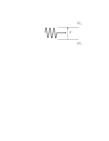
Figure 2: A two-level system illustrating an auxiliary SQUID. The coupling constant between the cavity field and auxiliary SQUID is $g^{\prime}$.

This the central idea of Kansas scheme, from which we can see that a post-selection measurement plays a key role in creating the flux qubit entanglement. The post-selection measurement is performed by an auxiliary SQUID. In the following, we consider the auxiliary SQUID as a part of whole quantum system.

III III. Dynamical evolution

In this section the auxiliary SQUID will be taken into account as a quantum subsystem. And the dynamical evolution of the measured system (two SQUIDs) will be considered. Together with the auxiliary SQUID, the whole system contains two parts, the auxiliary SQUID as the apparatus and the two SQUIDs as the measured system. Therefore, in the interaction picture, the Hamiltonian of the whole system reads as

$$H = H_{0}+H_{A}\text{,}$$ (6)

$$H_{A} = g^{\prime}c\left|e\right\rangle_{A}\left\langle g\right|+H.c.\text{.}$$

$H_{A}$ describes the interaction between the auxiliary SQUID and the cavity field with the coupling constant $g^{\prime}$. For simplicity, in the following we consider the case with the parameters

$$g_{1} = g_{2}=g\text{,}$$

$$\Omega_{1} = \Omega_{2}=\Omega\text{.}$$ (7)

Obviously, we have

$$[H,\mathcal{N}]=0,$$ (8)

where

$$\mathcal{N}=\sum_{l}\left(\left|a\right\rangle_{l}\left\langle a\right|+\left|1\right\rangle_{l}\left\langle 1\right|\right)+\left|a\right\rangle_{A}\left\langle a\right|+c^{\dagger}c.$$ (9)

When $g^{\prime}$ is switched off, the dark state $\left|d\right\rangle$ from (II) does not evolve since it is an eigenstate of $H_{0}$. When the auxiliary SQUID is employed to measure the state of the cavity field, $g^{\prime}$ is switched on, state $\left|d\right\rangle$ will evolve driven by the Hamiltonian (6). If the auxiliary SQUID is in the ground state $\left|g\right\rangle_{A}$ initially, while two-SQUID system is in the state $\left|d\right\rangle$, the initial state will evolve in the invariant subspace $V_{s}$ with $\mathcal{N}=1$, which is spanned by the following basis

$$\left|\varphi_{1}\right\rangle = \left|0\right\rangle_{I}\left|0\right\rangle_{II}\left|1\right\rangle_{c}\left|g\right\rangle_{A}\text{,}$$

$$\left|\varphi_{2}\right\rangle = \left|a\right\rangle_{I}\left|0\right\rangle_{II}\left|0\right\rangle_{c}\left|g\right\rangle_{A}\text{,}$$

$$\left|\varphi_{3}\right\rangle = \left|0\right\rangle_{I}\left|a\right\rangle_{II}\left|0\right\rangle_{c}\left|g\right\rangle_{A}\text{,}$$ (10)

$$\left|\varphi_{4}\right\rangle = \left|0\right\rangle_{I}\left|0\right\rangle_{II}\left|0\right\rangle_{c}\left|e\right\rangle_{A}\text{,}$$

$$\left|\varphi_{5}\right\rangle = \left|1\right\rangle_{I}\left|0\right\rangle_{II}\left|0\right\rangle_{c}\left|g\right\rangle_{A}\text{,}$$

$$\left|\varphi_{6}\right\rangle = \left|0\right\rangle_{I}\left|1\right\rangle_{II}\left|0\right\rangle_{c}\left|g\right\rangle_{A}\text{.}$$

The corresponding matrix of $H$ in the subspace $V_{s}$ is

$$H=\left(\begin{array}[]{cccccc}0&g&g&g^{\prime}&0&0\\ g&0&0&0&\Omega&0\\ g&0&0&0&0&\Omega\\ g^{\prime}&0&0&0&0&0\\ 0&\Omega&0&0&0&0\\ 0&0&\Omega&0&0&0\end{array}\right)\text{.}$$ (11)

Considering the symmetry the whole system due to the identity of two SQUIDs ($I$ and $II$), the $6\times 6$ matrix can be block-diagonalized under the new basis

$$\left|\chi_{1}^{\left(-\right)}\right\rangle = \frac{1}{\sqrt{2}}\left(\left|\varphi_{2}\right\rangle-\left|\varphi_{3}\right\rangle\right)\text{,}$$

$$\left|\chi_{2}^{\left(-\right)}\right\rangle = \frac{1}{\sqrt{2}}\left(\left|\varphi_{5}\right\rangle-\left|\varphi_{6}\right\rangle\right)\text{,}$$

$$\left|\chi_{1}^{\left(+\right)}\right\rangle = \left|\varphi_{1}\right\rangle\text{,}$$ (12)

$$\left|\chi_{2}^{\left(+\right)}\right\rangle = \frac{1}{\sqrt{2}}\left(\left|\varphi_{2}\right\rangle+\left|\varphi_{3}\right\rangle\right)\text{,}$$

$$\left|\chi_{3}^{\left(+\right)}\right\rangle = \left|\varphi_{4}\right\rangle\text{,}$$

$$\left|\chi_{4}^{\left(+\right)}\right\rangle = \frac{1}{\sqrt{2}}\left(\left|\varphi_{5}\right\rangle+\left|\varphi_{6}\right\rangle\right)\text{.}$$

The matrix of the Hamiltonian $H$ can be written as

$$H=H_{2}\oplus H_{4}\text{,}$$ (13)

where

$$H_{2}=\left(\begin{array}[]{cc}0&1\\ 1&0\end{array}\right)\text{,}$$ (14)

and

$$H_{4}=\left(\begin{array}[]{cccc}0&\sqrt{2}g&g^{\prime}&0\\ \sqrt{2}g&0&0&\Omega\\ g^{\prime}&0&0&0\\ 0&\Omega&0&0\end{array}\right)\text{.}$$ (15)

Here, $g$ and $g^{\prime}$ are rescaled by $\Omega$: $g/\Omega\rightarrow g$, $g^{\prime}/\Omega\rightarrow g^{\prime}$.

Diagonalizing two matrices, eigenvalues are obtained as

$$E_{1}^{\left(-\right)} = -1\text{,}$$

$$E_{2}^{\left(-\right)} = 1\text{,}$$

$$E_{1}^{\left(+\right)} = \frac{1}{\sqrt{2}}[\sqrt{\eta^{2}-4g^{\prime 2}}+\eta]^{\frac{1}{2}}\text{,}$$ (16)

$$E_{3}^{\left(+\right)} = \frac{1}{\sqrt{2}}[-\sqrt{\eta^{2}-4g^{\prime 2}}+\eta]^{\frac{1}{2}}\text{,}$$

$$E_{2}^{\left(+\right)} = -E_{1}\text{,}$$

$$E_{4}^{\left(+\right)} = -E_{3}\text{,}$$

where

$$\eta=1+2g^{2}+g^{\prime 2}.$$ (17)

In the antisymmetry basis: $\{\left|\chi_{n}^{\left(-\right)}\right\rangle\left|\text{ }n=1,2\right.\}$ and symmetry basis: $\{\left|\chi_{n}^{\left(+\right)}\right\rangle\left|\text{ }n=1,2,3,4\right.\}$, corresponding eigenstates are expressed as

$$\left|\Psi_{1}^{\left(-\right)}\right\rangle = \frac{1}{\sqrt{2}}\left(\left|\chi_{1}^{\left(-\right)}\right\rangle-\left|\chi_{2}^{\left(-\right)}\right\rangle\right)\text{,}$$

$$\left|\Psi_{2}^{\left(-\right)}\right\rangle = \frac{1}{\sqrt{2}}\left(\left|\chi_{1}^{\left(-\right)}\right\rangle+\left|\chi_{2}^{\left(-\right)}\right\rangle\right)\text{,}$$

$$\left|\Psi_{1}^{\left(+\right)}\right\rangle = N_{1}(\frac{E_{3}^{2}-1}{g}\left|\chi_{1}^{\left(+\right)}\right\rangle+\sqrt{2}E_{3}\left|\chi_{2}^{\left(+\right)}\right\rangle-\frac{E_{3}}{g^{\prime}}\frac{E_{5}^{2}-g^{\prime 2}}{g}\left|\chi_{3}^{\left(+\right)}\right\rangle+\sqrt{2}\left|\chi_{4}^{\left(+\right)}\right\rangle)\text{,}$$

$$\left|\Psi_{2}^{\left(+\right)}\right\rangle = N_{1}(\frac{E_{3}^{2}-1}{g}\left|\chi_{1}^{\left(+\right)}\right\rangle-\sqrt{2}E_{3}\left|\chi_{2}^{\left(+\right)}\right\rangle+\frac{E_{3}}{g^{\prime}}\frac{E_{5}^{2}-g^{\prime 2}}{g}\left|\chi_{3}^{\left(+\right)}\right\rangle+\sqrt{2}\left|\chi_{4}^{\left(+\right)}\right\rangle)\text{,}$$ (18)

$$\left|\Psi_{3}^{\left(+\right)}\right\rangle = N_{2}(\frac{E_{5}^{2}-1}{g}\left|\chi_{1}^{\left(+\right)}\right\rangle+\sqrt{2}E_{5}\left|\chi_{2}^{\left(+\right)}\right\rangle-\frac{E_{5}}{g^{\prime}}\frac{E_{3}^{2}-g^{\prime 2}}{g}\left|\chi_{3}^{\left(+\right)}\right\rangle+\sqrt{2}\left|\chi_{4}^{\left(+\right)}\right\rangle)\text{,}$$

$$\left|\Psi_{4}^{\left(+\right)}\right\rangle = N_{2}(\frac{E_{5}^{2}-1}{g}\left|\chi_{1}^{\left(+\right)}\right\rangle-\sqrt{2}E_{5}\left|\chi_{2}^{\left(+\right)}\right\rangle+\frac{E_{5}}{g^{\prime}}\frac{E_{3}^{2}-g^{\prime 2}}{g}\left|\chi_{3}^{\left(+\right)}\right\rangle+\sqrt{2}\left|\chi_{4}^{\left(+\right)}\right\rangle)\text{,}$$

where $N_{1}$ and $N_{2}$ are normalized factors.

Now, the dynamical evolution of the initial state

$$\left|d\left(0\right)\right\rangle = N(g\left|1\right\rangle_{I}\left|0\right\rangle_{II}\left|0\right\rangle_{c}+g\left|0\right\rangle_{I}\left|1\right\rangle_{II}\left|0\right\rangle_{c}-\left|0\right\rangle_{I}\left|0\right\rangle_{II}\left|1\right\rangle_{c})\left|g\right\rangle_{A}$$ (19)

$$= N\left(\sqrt{2}g\left|\chi_{4}^{\left(+\right)}\right\rangle-\left|\chi_{1}^{\left(+\right)}\right\rangle\right)\text{,}$$

where $N=1/\sqrt{2g^{2}+1}$ normalized factor, can be calculated. From (19) we find that $\left|d\left(0\right)\right\rangle$ is in the symmetrical subspace. At time $t$, it evolves into

$$\left|d\left(t\right)\right\rangle = F_{1}\left(t\right)\left|\chi_{1}^{\left(+\right)}\right\rangle+F_{2}\left(t\right)\left|\chi_{2}^{\left(+\right)}\right\rangle+F_{3}\left(t\right)\left|\chi_{4}^{\left(+\right)}\right\rangle+F_{4}\left(t\right)\left|\chi_{3}^{\left(+\right)}\right\rangle$$

$$= F_{1}\left(t\right)\left|0\right\rangle_{I}\left|0\right\rangle_{II}\left|1\right\rangle_{c}\left|g\right\rangle_{A}+F_{2}\left(t\right)\left|D\right\rangle\left|0\right\rangle_{c}\left|g\right\rangle_{A}$$

$$+F_{3}\left(t\right)\left|C\right\rangle\left|0\right\rangle_{c}\left|g\right\rangle_{A}+F_{4}\left(t\right)\left|0\right\rangle_{I}\left|0\right\rangle_{II}\left|0\right\rangle_{c}\left|e\right\rangle_{A}\text{,}$$

where

$$F_{1}\left(t\right) = 2N\left(t\right)[N_{1}^{2}\frac{E_{3}^{2}-1}{g}X\cos\left(E_{3}t\right)+Z\frac{E_{5}^{2}-1}{g}\cos\left(E_{5}t\right)]\text{,}$$

$$F_{2}\left(t\right) = -i2\sqrt{2}N\left(t\right)[N_{1}^{2}E_{3}X\sin\left(E_{3}t\right)+ZE_{5}Y\sin\left(E_{5}t\right)]\text{,}$$

$$F_{3}\left(t\right) = 2\sqrt{2}N\left(t\right)[N_{1}^{2}X\cos\left(E_{3}t\right)+ZY\cos\left(E_{5}t\right)]\text{,}$$ (21)

$$F_{4}\left(t\right) = i2N\left(t\right)[\frac{N_{1}^{2}E_{3}}{g^{\prime}}\frac{E_{5}^{2}-g^{\prime 2}}{g}X\sin\left(E_{3}t\right)+ZE_{5}\frac{E_{3}^{2}-g^{\prime 2}}{gg^{\prime}}Y\sin\left(E_{5}t\right)]\text{,}$$

and

$$X = 2g-\frac{E_{3}^{2}-1}{g}\text{,}$$

$$Y = 2g-\frac{E_{5}^{2}-1}{g}\text{,}$$

$$Z = \frac{1}{4}-N_{1}^{2}\text{,}$$ (22)

$$\left|D\right\rangle = \frac{1}{\sqrt{2}}\left(\left|a\right\rangle_{I}\left|0\right\rangle_{II}+\left|0\right\rangle_{I}\left|a\right\rangle_{II}\right)\text{,}$$

$$\left|C\right\rangle = \frac{1}{\sqrt{2}}\left(\left|1\right\rangle_{I}\left|0\right\rangle_{II}+\left|0\right\rangle_{I}\left|1\right\rangle_{II}\right)\text{,}$$

where $N\left(t\right)$ is the normalized factor.

Some observations follow: (1) States $\left|g\right\rangle_{A}$ and $\left|e\right\rangle_{A}$ of the auxiliary SQUID are entangled with states of two SQUIDs and the cavity field; (2) When the measurement to the auxiliary SQUID is carried out, the auxiliary SQUID will collapse into a quantum state. If the auxiliary SQUID collapses to the ground state $\left|g\right\rangle_{A}$, one can not determine which state two SQUIDs will be in. This is because there exist three states ($\left|0\right\rangle_{I}\left|0\right\rangle_{II}$, $\left|C\right\rangle$, and $\left|D\right\rangle$) of two SQUIDs entangled with state $\left|g\right\rangle_{A}$. In the following section, we will discuss how to create the entangled state $\left|C\right\rangle$ by choosing optimal parameters.

IV IV. Creating maximally entangled state by optimizing parameters

There exist two entangled states $\left|C\right\rangle$ and $\left|D\right\rangle$ in state $\left|d\left(t\right)\right\rangle$. In this paper, $\left|C\right\rangle$ is the target state in accordance with Ref. Yang . The entangled state $\left|D\right\rangle$ contains excited states $\left|a\right\rangle_{l}$ of two SQUIDs, which couple to the environment with a higher probability of transitions to the first excited state $\left|1\right\rangle_{l}$ or the ground state $\left|0\right\rangle_{l}$, so state $\left|D\right\rangle$ is unstable. Therefore, state $\left|C\right\rangle$ is a good candidate for quantum information process.

To create entangled state $\left|C\right\rangle$, we first choose a special instant $t_{0}$ to satisfy

$$P_{1}\left(t_{0}\right)=P_{2}\left(t_{0}\right)=0\text{,}$$ (23)

where $P_{1}\left(t_{0}\right)=\left|F_{1}\left(t_{0}\right)\right|^{2}$ and $P_{2}\left(t_{0}\right)=\left|F_{2}\left(t_{0}\right)\right|^{2}$. The above equations can be regarded “entanglement condition”, which introduce the relation between $E_{3}$ and $E_{5}$. The parameters can be determined when $P_{3}\left(t_{0}\right)=\left|F_{3}\left(t_{0}\right)\right|^{2}$, which is the probability of state $\left|C\right\rangle\left|0\right\rangle_{c}\left|g\right\rangle_{A}$, reaches its maximum. Then the entangled state $\left|C\right\rangle$ can be generated with higher success probability. Based on the entanglement condition (23), numerical simulations are employed to find the maximal value of $P_{3}\left(E_{3}\right)$. Numerical results are listed in Figs. 3, 4.

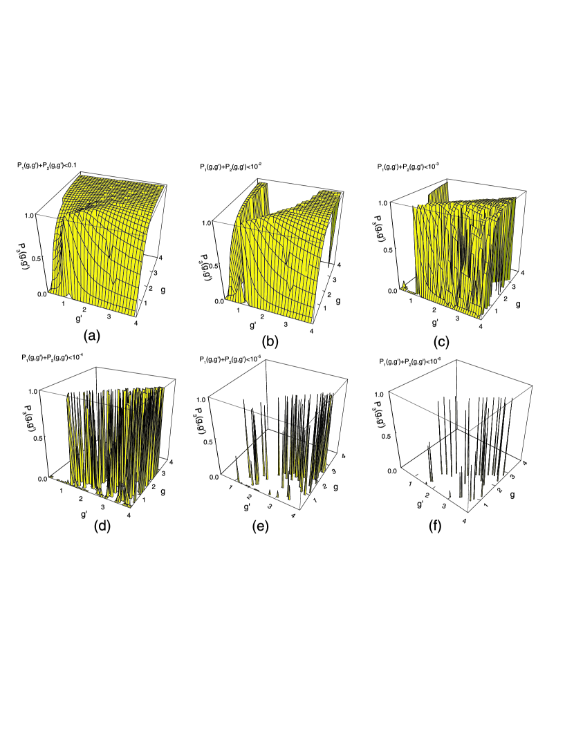
Figure 3: The relation between maximal values of $P_{3}$ and $g$ as well as $g^{\prime}$ when $P_{1}+P_{2}<10^{-i}$($i=1,2,...6$). The influence of the auxiliary SQUID is taken into account as a quantum subsystem. As a result the parameter $g$ of two SQUIDs and the parameter $g^{\prime}$ of the auxiliary SQUID must match so that the target entangled state can be induced. Numerical results show that the closer to the entanglement condition are the results the less is the number of $g$ and $g^{\prime}$.

As shown in Fig. 3, when $P_{1}\left(t_{0}\right)+P_{2}\left(t_{0}\right)$ is less than $10^{-j}$ ($j=1\sim 6$), the maximal values of $P_{3}\left(t_{0}\right)$ and magnitudes of $g$ and $g^{\prime}$ corresponding to these $P_{3}\left(t_{0}\right)$ are given respectively. Here, the influence of the auxiliary SQUID is taken into account as a quantum subsystem. As a result the parameter $g$ of the two SQUIDs and the parameter $g^{\prime}$ of the auxiliary SQUID must match so that the entangled state we need can be induced. The numerical results show that as $P_{1}\left(t_{0}\right)+P_{2}\left(t_{0}\right)$ approaches to vanishing, the optimal area in $gg^{\prime}$ plane, within which $P_{3}\left(t_{0}\right)$ closes to unit.

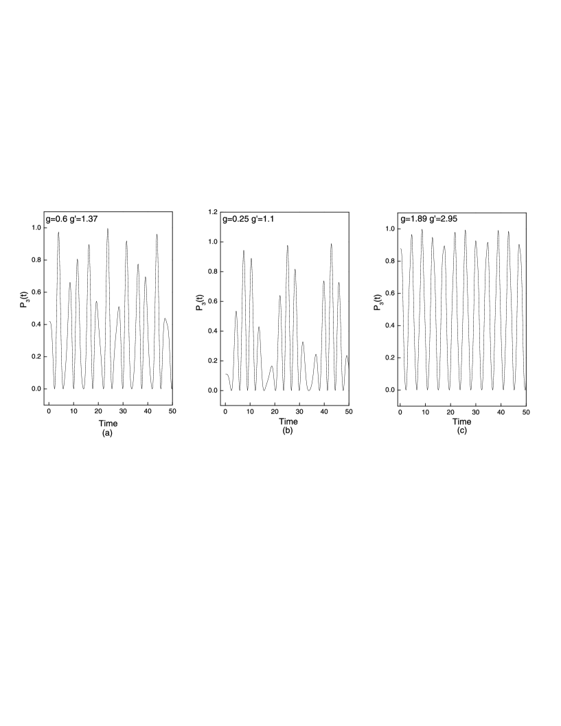
Figure 4: The relation between time and $P_{3}\left(t\right)$. In the case of $P_{1}\left(t_{0}\right)+P_{2}\left(t_{0}\right)$ less than $10^{-6}$, three groups $g$ and $g^{\prime}$ are chosen. Numerical results show that $t_{0}$ which make $P_{3}\left(t_{0}\right)$ maximal is not $\pi/g^{\prime}$ due to the back reaction of the auxiliary SQUID to two SQUIDs.

We also investigate the dynamical process of the entanglement creation by numerical simulation. For the case with fixed $g$ and $g^{\prime}$, under the condition $P_{1}\left(t_{0}\right)+P_{2}\left(t_{0}\right)\leq 10^{-6}$, the time evolution of $P_{3}\left(t\right)$ is calculated.

Three groups of $g\$and $g^{\prime}$ with $(g,\ g^{\prime})=(0.25,$ $1.89),$ $(2.95,$ $1.10),$ $(0.60,$ $1.37)$ are chosen to demonstrate the dynamical process of the creation of entanglement. Corresponding initial states are $\left|d\left(0\right)\right\rangle=$ $N\left(\sqrt{2}g\left|\chi_{4}^{\left(+\right)}\right\rangle-\left|\chi_{1}^{\left(+\right)}\right\rangle\right)$ with $N=1/\sqrt{2g^{2}+1}$. In each case, the component of maximal entangled state in the initial state is $2g^{2}/N^{2}$. Numerical results are plotted in Fig. 4. Taking Fig. 4(b) as an example, the initial state is the dark state of the two SQUIDs, which contains a small component ($\sim 0.11$) of the maximal entangled state. When the coupling to the auxiliary SQUID is switched on, i.e., $g^{\prime}=0\longrightarrow 1.10$, to probe the state of the cavity field. After $t_{0}$, the quantum state which contains a maximal component of state $\left|C\right\rangle$ is generated. Then the post selection measurement to the auxiliary SQUID is carried out. As a result of maximizing the probability $P_{3}\left(t_{0}\right)$, there exits very large probability to induce the state $\left|C\right\rangle$. This can also be found from Fig. 4(a,c). It indicates that the smaller component of state $\left|C\right\rangle$ is contained in the initial state, the longer time period $t_{0}$ is taken. Numerical results also show that period $t_{0}$ at which $P_{3}\left(t_{0}\right)$ gets maximum is no longer $\pi/g^{\prime}$ due to the back reaction of the auxiliary SQUID to the two SQUIDs.

V V. Summary

In this paper, the back action of the auxiliary SQUID to the two SQUIDs was taken into account in the theoretical scheme for creating the entangled state. The dynamical evolution of the two SQUIDs dark state (II) driven by the Hamiltonian of two SQUIDs together with the auxiliary SQUID is calculated precisely. By using the entanglement condition, the relation between parameters ($g$ and $g^{\prime}$) and the evolution time $t_{0}$ is determined. At instant $t_{0}$, the system reaches state $\left|d\left(t\right)\right\rangle=F_{3}\left(t\right)\left|C\right\rangle\left|0\right\rangle_{c}\left|g\right\rangle_{A}+F_{4}\left(t\right)\left|0\right\rangle_{I}\left|0\right\rangle_{II}\left|0\right\rangle_{c}\left|e\right\rangle_{A}$. By optimizing the parameters ($g$ and $g^{\prime}$), the probability $P_{3}\left(t_{0}\right)=\left|F_{3}\left(t_{0}\right)\right|^{2}$ of the entangled state $\left|C\right\rangle$ is maximized at $t_{0}$. After the post selection measurement for the auxiliary SQUID, entangled state $\left|C\right\rangle$ is feasibly induced. Numerical results show that the period $t_{0}$ given by the entanglement condition is not $\pi/g^{\prime}$. This is because the auxiliary SQUID is taken into account as a quantum subsystem.

We gratefully acknowledge the valuable discussion with Professor Chang-Pu Sun. This work is supported by the CNSF (Grant No. 10474104), the National Fundamental Research Program of China (No. 2001CB309310).

References

• (1) Y. Makhlin, G. Schoen, and A. Shnirman, Nature (London) 398, 305 (1999).
• (2) Y. Nakamura, Y. Pashkin, and J.S. Tsai, Nature (London) 398, 786 (1999).
• (3) R. Rouse, S. Han, and J.E. Lukens, Phys. Rev. Lett. 75, 1614 (1995).
• (4) S. Han, R. Rouse, and J.E. Lukens, Phys. Rev. Lett. 76, 3404 (1996).
• (5) Z. Zhou, S.-I. Chu, and S. Han, Phys. Rev. B 73, 104521 (2006).
• (6) C.-P. Yang, S.-I. Chu, and S. Han, Phys. Rev. A 67, 042311 (2003).
• (7) C.-P. Yang, S.-I. Chu, and S. Han, Phys. Rev. Lett. 92, 117902 (2004).
• (8) Z. Zhou, S.-I. Chu, and S. Han, Phys. Rev. B 70, 094513 (2004).
• (9) Zsolt Kis and Emmanuel Paspalakis, Phys. Rev. B. 69, 024510 (2004).
• (10) A. Steinbach et al., Phys. Rev. Lett. 87, 137003 (2001).
• (11) Yu.A. Pashkin et al., Nature (London) 421, 823 (2003).
• (12) A.J. Berkley et al., Science 300, 1548 (2003).
• (13) Y. Makhlin, G. Schon, and A. Shnirman, Rev. Mod. Phys. 73, 357 (2001).
• (14) J.Q. You, J.S. Tsai, and F. Nori, Phys. Rev. B 68, 024510 (2003).
• (15) J.Q. You, J.S. Tsai, and F. Nori, Phys. Rev. Lett. 89, 197902 (2002).