Channel simulation with quantum side information

Abstract

We study and solve the problem of classical channel simulation with quantum side information at the receiver. This is a generalization of both the classical reverse Shannon theorem, and the classical-quantum Slepian-Wolf problem. The optimal noiseless communication rate is found to be reduced from the mutual information between the channel input and output by the Holevo information between the channel output and the quantum side information.

Our main theorem has two important corollaries. The first is a quantum generalization of the Wyner-Ziv problem: rate-distortion theory with quantum side information. The second is an alternative proof of the trade-off between classical communication and common randomness distilled from a quantum state.

The fully quantum generalization of the problem considered is quantum state redistribution. Here the sender and receiver share a mixed quantum state and the sender wants to transfer part of her state to the receiver using entanglement and quantum communication. We present outer and inner bounds on the achievable rate pairs.

1 Introduction

In his seminal 1948 paper [24] Shannon introduced the problem of data compression. He found that a memoryless source consisting of a large number $n$ of symbols generated according to a probability distribution $p$ can be compressed without loss at a rate of $H(p)$ bits per symbol, where $H(p)$ is the Shannon entropy of $p$. This result can be rephrased as a communication problem. The sender Alice wants to communicate her source to the receiver Bob. Equivalently, she wants to simulate a noiseless bit channel (which we denote by $\overline{\operatorname{id}}$) from her to Bob with respect to the input $p$. She can accomplish this task by using up a rate $H(p)$ of perfect bit channels (which we denote by $[c\rightarrow c]$) from her to Bob. The protocol consists of Alice sending the compressed source and Bob performing decompression upon receipt. The existence of such a protocol may be succinctly expressed as a resource inequality [10, 15, 11]

$$H(p)\,[c\rightarrow c]\geq\langle\overline{\operatorname{id}}:p\rangle.$$

The non-local resource on the left hand side can be composed with local pre- and post-processing to simulate the non-local resource on the right hand side.

With this viewpoint in mind, Shannon’s result was generalized some 50 years later to simulating noisy channels. The latter result was dubbed the reverse Shannon theorem  [5, 27], referring to Shannon’s noisy channel coding theorem [24]. One may well ask why one should be interested in simulating noise. The reason is a saving in resources: part of the classical communication $[c\rightarrow c]$ can be replaced by shared coins or “common randomness” (denoted by $[c\,c]$). Common randomness is a strictly weaker resource than classical communication because Alice can flip her coin locally and send the outcome to Bob. The reverse Shannon theorem is intimately related [27] to lossy compression, or rate-distortion theory [6], where the communication rate is traded off against a suitably defined distortion level of the data. More generally, the reverse Shannon theorem is a useful tool for effecting trade-offs between resources [18, 4] .

Another generalization of Shannon’s result, introduced by Slepian and Wolf [25], is to give Bob side information about source. The case of quantum side information was considered in [14].

In this paper we combine the two ideas of making the channel noisy and allowing quantum side information with the receiver. We also analyze several consequences for trade-offs. The first is rate-distortion theory with quantum side information paralleling the classical work of Wyner and Ziv [29]. The second is an alternative derivation of a result from  [15] concerning distillation of common randomness from a bipartite quantum state with the assistance of one-way classical communication. The various implications of our result are shown in Figure 1.

This paper is organized as follows. In Section 2 we introduce the notation and give some background. Section 3 contains our main result, Theorem 3.1, together with its proof. Section 4 discusses consequences of Theorem 3.1. In section 5 we find outer and inner bounds for a fully quantum version of our problem. Section 6 concludes with a discussion and proposed future work.

Figure 1: The relation of our results to prior work.

2 Notation

Let us introduce some useful notation for the bipartite classical-quantum systems. The state of a classical-quantum system $XB$ can be described by an ensemble ${\cal E}=\{\rho^{B}_{x},p(x)\}$, with $p(x)$ defined on ${\cal X}$ and the $\rho^{B}_{x}$ being density operators on the Hilbert space ${\cal H}_{B}$ of $B$. Thus, with probability $p(x)$ the classical index and quantum state take on values $x$ and $\rho^{B}_{x}$, respectively. A useful representation of classical-quantum systems is obtained by embedding the random variable $X$ in some quantum system, also labelled by $X$. Then our ensemble $\{\rho^{B}_{x},p(x)\}$ corresponds to the density operator

$$\rho^{XB}=\sum_{x}p(x)|x\rangle\langle x|^{X}\otimes\rho^{B}_{x},$$ (1)

where $\{|x\rangle:x\in{\cal X}\}$ is an orthonormal basis for the Hilbert space ${\cal H}_{X}$ of $X$. A classical-quantum system may, therefore, be viewed as a special case of a quantum one. The von Neumann entropy of a quantum system $A$ with density operator $\sigma^{A}$ is defined as $H(A)_{\sigma}=-\operatorname{Tr}{\sigma^{A}\log{\sigma^{A}}}$. The subscript is often omitted. For a tripartite quantum system $ABC$ in some state $\sigma^{ABC}$ define the conditional von Neumann entropy

$$H(B|A)=H(AB)-H(A),$$

quantum mutual information

$$I(A;B)=H(A)+H(B)-H(AB)=H(B)-H(B|A),$$

and quantum conditional mutual information

$$I(A;B|C)=I(A;BC)-I(A;C).$$

For classical-quantum correlations (1) the von Neumann entropy $H(X)_{\rho}$ is just the Shannon entropy $H(X)=-\sum_{x}p(x)\log{p(x)}$ of the random variable $X$. The conditional entropy $H(B|X)$ equals $\sum_{x}p(x)H(\rho^{B}_{x})$. The mutual information $I(X;B)$ is the Holevo quantity [19] of the ensemble ${\cal E}$:

$$\chi({\cal E})=H\left(\sum_{x}p(x)\rho_{x}\right)-\sum_{x}p(x)H(\rho_{x}).$$

Finally we need to introduce a classical-quantum analogue of a Markov chain. We may define a classical-quantum Markov chain $Y\!{\,\rightarrow\,}\!X{\,\rightarrow\,}\!B$ associated with an ensemble $\{\rho^{B}_{xy},p(x,y)\}$ for which $\rho^{B}_{xy}=\rho^{B}_{x}$ is independent of $y$. Such an object typically comes about by augmenting the system $XB$ by the random variable $Y$ (classically) correlated with $X$ via a conditional distribution $W(y|x)=\Pr\{Y=y|X=x\}$. This corresponds to the state

$$\rho^{XYB}=\sum_{x}p(x)\sum_{y}W(y|x)|y\rangle\langle y|^{Y}\otimes|x\rangle\langle x|^{X}\otimes\rho_{x}^{B}.$$ (2)

Here $W(y|x)$ is the noisy channel and $X$ and $Y$ are input and output random variables. Therefore the classical-quantum system $YB$ can be expressed as

$$\rho^{YB}=\sum_{y}q(y)|y\rangle\langle y|^{Y}\otimes\rho_{y}^{B}$$ (3)

with $q(y)=\sum_{x}p(x)W(y|x)$ and $\rho_{y}^{B}=\sum_{x}P(x|y)\rho_{x}^{B}$.

3 Channel simulation with quantum side information

Consider a classical-quantum system $XB$ in the state (1) such that the sender Alice possesses the classical index $X$ and the receiver Bob has the quantum system $B$. Consider a classical channel from Alice to Bob given by the conditional probability distribution $W$. Applying this channel to the $X$ part of $\rho^{XB}$ results in the state $\rho^{XYB}$ given by (2). Ideally, we are interested in simulating the channel $W$ using noiseless communication and common randomness, in the sense that the simulation produces the state $\rho^{XYB}$. For reasons we will discuss later, we want Alice to also get a copy $\overline{Y}$ of the output, so that the final state produced is

$$\rho^{XY\overline{Y}B}=\sum_{x}p(x)\sum_{y}W(y|x)|y\rangle\langle y|^{Y}\otimes|y\rangle\langle y|^{\overline{Y}}\otimes|x\rangle\langle x|^{X}\otimes\rho_{x}^{B}.$$ (4)

The systems $X$ and $\overline{Y}$ are in Alice’s possession, while Bob has $B$ and $Y$.

As usual in information theory, this task is amenable to analysis when we go to the approximate, asymptotic i.i.d. (independent, identically distributed) setting. This means that Alice and Bob share $n$ copies of the classical-quantum system $XB$, given by the state

$$\rho^{X^{n}B^{n}}=\sum_{x^{n}}p^{n}(x^{n})|x^{n}\rangle\!\langle x^{n}|^{X^{n}}\otimes\rho^{B^{n}}_{x^{n}},$$ (5)

where $x^{n}=x_{1}\dots x_{n}$ is a sequence in ${\cal X}^{n}$, $p^{n}(x^{n})=p(x_{1})\dots p(x_{n})$, and $\rho_{x^{n}}=\rho_{x_{1}}\otimes\rho_{x_{2}}\cdots\otimes\rho_{x_{n}}$. They want to simulate the channel $W^{n}(y^{n}|x^{n})=W(y_{1}|x_{1})\dots W(y_{n}|x_{n})$ approximately, with error approaching zero as $n\rightarrow\infty$. They have access to a rate of $C$ bits/copy of common randomness, which means that they have the same string $l$ picked uniformly at random from the set $\{0,1\}^{nC}$. In addition, they are allowed a rate of $R$ bits/copy of classical communication, so that Alice may send an arbitrary string $m$ from the set $\{0,1\}^{nR}$ to Bob.

An $(n,R,C,\epsilon)$ simulation code consists of

• An encoding stochastic map $E_{n}:{\cal X}^{n}\times\{0,1\}^{nC}\rightarrow\{0,1\}^{nR}\times\{0,1\}^{nS}$. If the value of the common randomness is $l\in\{0,1\}^{nC}$, Alice encodes her classical message $x^{n}$ as the index $ms$, $m\in\{0,1\}^{nR}$, $s\in\{0,1\}^{nS}$, with probability $E_{l}(m,s|x^{n}):=E_{n}(m,s|x^{n},l)$, and only sends $m$ to Bob;

• A set $\{\Lambda^{(lm)}\}_{lm\in\{0,1\}^{n(C+R)}}$, where each $\Lambda^{(lm)}=\{\Lambda^{(lm)}_{s^{\prime}}\}_{s^{\prime}\in\{0,1\}^{nS}}$ is a POVM acting on $B^{n}$ and taking on values $s^{\prime}$. Bob does not get sent the true value of $s$ and needs to infer it from the POVM;

• A deterministic decoding map $D_{n}:\{0,1\}^{nC}\times\{0,1\}^{nR}\times\{0,1\}^{nS}\rightarrow{\cal Y}^{n}$; this allows Alice and Bob to produce their respective simulated outputs $\widetilde{y}^{n}=D_{l}(m,s):=D_{n}(l,m,s)$ and $\hat{y}^{n}=D_{l}(m,s^{\prime})$, based on $l$, $m$ and $s$ (in Bob’s case $s^{\prime}$);

such that

$$\|(\rho^{XY\overline{Y}B})^{\otimes n}-\sigma^{X^{n}\hat{Y}^{n}\widetilde{Y}^{n}\hat{B}^{n}}\|_{1}\leq\epsilon.$$ (6)

Here the state $\sigma^{X^{n}\hat{Y}^{n}\widetilde{Y}^{n}\hat{B}^{n}}$ denotes the result of the simulation, which includes Alice’s original $X^{n}$, the post-measurement system $\hat{B}^{n}$, Alice’s simulation output random variable $\widetilde{Y}^{n}$ and Bob’s simulation output random variable $\hat{Y}^{n}$ (based on $s^{\prime}$).

A rate pair $(R,C)$ is called achievable if for all $\epsilon>0$, $\delta>0$ and sufficiently large $n$, there exists an $(n,R+\delta,C+\delta,\epsilon)$ code.

We now state our main theorem.

Theorem 3.1

The region of achievable $(R,C)$ pairs is given by

$$R\geq I(X;Y)-I(Y;B),\quad\quad C+R\geq H(Y|B).$$

The theorem contains a direct coding part (achievability) and a converse part (optimality). For the direct coding theorem it suffices to prove the achievability of the rate pair $(R,C)=(I(X;Y)-I(Y;B),H(Y|X))$. The full region given by Theorem 3.1 (see Figure 2) follows by observing that a bit of common randomness may be generated from a bit of communication.

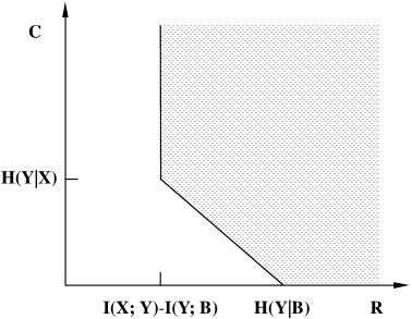
Figure 2: Achievable region of rate pairs for a classical-quantum system $XB$.

A naive simulation would be for Alice to actually perform the channel $W$ locally and send a compressed instance of the output to Bob. This would require a communication rate of $H(Y)$ bits per copy. The first idea is to split this information into an intrinsic and extrinsic part [28]. The extrinsic part has rate $H(Y|X)$ and is provided by the common randomness. Only the intrinsic part $I(X;Y)=H(Y)-H(Y|X)$ requires classical communication. This protocol would amount to sending the strings $m$ and $s$ above. However, a further savings of $I(Y;B)$ is accomplished by Bob deducing the $s$ index from his quantum state. Thus Alice need only send $m$ which requires a rate $I(X;Y)-I(Y;B)$.

For the direct coding part we will need several lemmas. The first one is the Chernoff bound (cf. [2]).

Lemma 3.2 (Chernoff bound)

Let $Z_{1},\dots,Z_{n}$ be i.i.d. random variables with mean $\mu$. Define $\overline{Z}_{n}=\frac{1}{n}\sum_{j=1}^{n}Z_{j}$. If the $Z_{j}$ take values in the interval $[0,b]$, then for $\eta\leq\frac{1}{2}$, and some constant $\kappa_{0}$,

$$\Pr\{|\overline{Z}_{n}-\mu|\geq\mu\eta\}\leq 2\exp(-\kappa_{0}n\mu\eta^{2}/b).$$ (7)

The second lemma concerns deterministically “diluting” a uniformly distributed random variable to a non-uniform one on a larger set. We will need it to create $y^{n}$ from $l$, $m$ and $s$.

Lemma 3.3 (Randomness dilution)

We are given a probability distribution $q(y)$ defined on ${\cal Y}$ and a set ${\cal T}\subseteq{\cal Y}$ such that

$$q({\cal T}) :=\sum_{y\in{\cal T}}q(y)\geq 1-\epsilon,$$ (8)

$$q(y) \geq\alpha,\,\,\,\forall y\in{\cal T},$$ (9)

for some positive numbers $\alpha$ and $\epsilon$. Let $W$ be the random variable uniformly distributed on $\{1,\ldots,M\}$. For random variables $Y_{1},Y_{2},...,Y_{M}$ all distributed according to $q$, define the map $G:\{1,...,M\}\rightarrow{\cal Y}$ by $G(i)=Y_{i}$. Then, letting $\widetilde{q}$ be the distribution of $G(W)$,

$$\Pr\{\|q-\widetilde{q}\|_{1}\geq\eta+\epsilon\}\leq 2|{\cal T}|\exp(-\kappa_{0}M\alpha\eta^{2})$$

for some constant $\kappa_{0}$.

Proof  Consider the indicator function $I(G(i)=y)$ taking values in $\{0,1\}$. Observe that $I(G(i)=y)$ for $i\in\{1,...,M\}$ are i.i.d. random variables with expectation value $\mathbb{E}I(G(i)=y)=q(y).$ The distribution $\widetilde{q}(y)$ of $G(W)$ is $\frac{1}{M}\sum_{i=1}^{M}I(G(i)=y)$. By the Chernoff bound (7), for each $y\in{\cal T}$, for $\eta\leq\frac{1}{2}$, and some constant $\kappa_{0}$,

$$\Pr\left\{\left|\frac{1}{M}\sum_{i=1}^{M}I(G(i)=y)-q(y)\right|\geq q(y)\eta\right\}\leq 2\exp(-\kappa_{0}M\alpha\eta^{2}).$$ (10)

By the union bound,

$$\Pr\{{\rm not}\,\,\iota\}\leq 2|{\cal T}|\exp(-\kappa_{0}M\alpha\eta^{2}),$$

where the logic statement $\iota$ is given by

$$\iota=\left\{\widetilde{q}\in[\hat{q}(1-\eta),\hat{q}(1+\eta)]\right\}$$

and $\hat{q}(y)=q(y)I(y\in{\cal T})$. It remains to relate $\iota$ to a statement about $\|\widetilde{q}-q\|_{1}$. First observe that

$$\begin{split}\|\hat{q}-q\|_{1}&=\sum_{y}|\hat{q}(y)-q(y)|\\ &=\sum_{y\not\in{\cal T}}q(y)\leq\epsilon.\end{split}$$ (11)

Second, observe that $\iota$ implies $\|\widetilde{q}-\hat{q}\|_{1}\leq\eta.$ The two give, via the triangle inequality

$$\|q-\widetilde{q}\|_{1}\leq\eta+\epsilon.$$

The statement of the lemma follows. $\Box$

Corollary 3.4

Consider a random variable $Y$ with distribution $q(y)$, and let $W$ be the random variable uniformly distributed on $\{1,\ldots,M\}$. For random variables $Y_{1},Y_{2},...,Y_{M}$ all distributed according to $q^{n}$, define the map $G:\{1,...,M\}\rightarrow{\cal Y}^{n}$ by $G(i)=Y_{i}$. Let $\widetilde{q}$ be the distribution of $G(W)$. Then, for all $\epsilon,\delta>0$ and sufficiently large $n$,

$$\Pr\{\|q^{n}-\widetilde{q}\|_{1}\geq 2\epsilon\}\leq 2\gamma\exp(-\kappa_{0}M\epsilon^{2}/\gamma),$$

where $\gamma=2^{n[H(Y)+c\delta]}$ and $c$ is some positive constant.

Proof  We will assume familiarity with the properties of typicality and conditional typicality, collected in the Appendix. We can relate to Lemma 3.3 through the identifications: ${\cal Y}\rightarrow{\cal Y}^{n}$, $q(y)\rightarrow{q}^{n}(y^{n})$, and ${\cal T}\rightarrow{{\cal T}}^{n}_{Y,\delta}$. The two conditions now read

$$q^{n}({\cal T}^{n}_{Y,\delta}) \geq 1-\epsilon,$$ (12)

$${q^{n}}(y^{n}) \geq\gamma^{-1},\,\,\,\forall y^{n}\in{\cal T}^{n}_{Y,\delta}.$$ (13)

These follow from properties $1$ and $2$ of Theorem A.1 (relabeling $X$ to $Y$ and $p$ to $q$).

$\Box$

Our next lemma contains the crucial ingredient of the direct coding theorem and is based on [28]. It will tell us how to define the encoding and decoding operations for a particular value of the common randomness.

Lemma 3.5 (Covering lemma)

We are given a probability distribution $q(y)$ and a conditional probability distribution $P(x|y)$, with $x\in{\cal X}$ and $y\in{\cal Y}$. Assume the existence of sets ${\cal T}\subseteq{\cal X}$ and $({\cal T}_{y})_{y\in{\cal Y}}\subseteq{\cal X}$ with the following properties for all $y\in{\cal Y}$:

$$\sum_{y\in{\cal Y}}q(y)P({\cal T}_{y}|y)\; \geq\;1-\epsilon,$$ (14)

$$\sum_{y\in{\cal Y}}q(y)P({\cal T}|y)\; \geq\;1-\epsilon,$$ (15)

$$|{\cal T}|\; \leq\;K,$$ (16)

$$P(x|y)\; \leq\;k^{-1},\quad\quad\forall x\in{\cal T}_{y}.$$ (17)

Define $M=\left\lceil\eta^{-1}K/k\right\rceil$ for some $0<\eta<1$. Given random variables $Y_{1},Y_{2},...,Y_{M}$ all distributed according to $q$, define the map $D:\{1,2,...,M\}\rightarrow{\cal Y}$ by $D(i)=Y_{i}$. Then there exists a conditional probability distribution $E(i|x)$ defined for $i\in\{1,2,...,M\}$ such that

$$\Pr\{\|\hat{P}u-Ep\|_{1}\geq 5\epsilon\}\leq 2K\exp(-\kappa_{0}\epsilon^{3}/\eta),$$ (18)

where $\hat{P}(x|i)=P(x|D(i))$, $u$ is the uniform distribution on $\{1,2,...,M\}$ and $p$ is the marginal distribution defined by $p(x)=\sum_{y\in{\cal Y}}P(x|y)q(y)$.

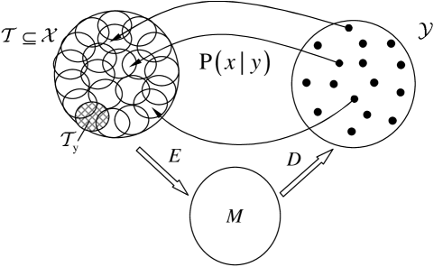
Figure 3: The covering lemma.

Remark  The meaning of the covering lemma is illustrated in Figure 3. A uniform distribution on the set $\{1,2,...,M\}$ is diluted via the map $D$ to the set ${\cal Y}$, and then stochastically mapped to the set ${\cal X}$ via $P(x|y)$. Condition (18) says that the very same distribution on $\{1,2,...,M\}\times{\cal X}$ can be obtained by starting with the marginal $p(x)$ and stochastically “concentrating” it to the set $\{1,2,...,M\}$. For this to be possible, the conditional outputs of the channel $P(x|y)$ (for particular values of $y$) should be sufficiently spread out to cover the support of $p(x)$. Each conditional output random variable is supported on ${\cal T}_{y}$ (14) of cardinality roughly $\geq k$ (17), and $p(x)$ is supported on ${\cal T}$ (15) of cardinality $\leq K$ (16). Thus roughly $M\approx K/k$ conditional random variables $\hat{P}(x|i)$ should suffice for the covering.

Proof  The idea is to use the Chernoff bound, as in the proof of the randomness dilution lemma. First we trim our conditional distributions to make them fit the conditions of the Chernoff bound; the resulting bound is then related to the condition (18).

Define

$$w(x)=\sum_{y\in{\cal Y}}q(y)P(x|y)I(x\in{\cal A}_{y}),$$

with ${\cal A}_{y}={\cal T}_{y}\bigcap{\cal T}$ and ${\cal A}=\bigcup_{y\in{\cal Y}}{\cal A}_{y}$. By properties (14) and (15), $w({\cal A})=\sum_{y\in{\cal Y}}q(y)P({\cal A}_{y}|y)\geq 1-2\epsilon$. Further define ${\cal B}_{y}={\cal A}_{y}\bigcap\{x:w(x)\geq\epsilon/K\}$ and ${\cal B}=\bigcup_{y\in{\cal Y}}{\cal B}_{y}$. Then define

$$\widetilde{P}(x|y)=P(x|y)I(x\in{\cal B}_{y}),\quad\quad\widetilde{w}(x)=\sum_{y\in{\cal Y}}q(y)\widetilde{P}(x|y)=w(x)I(w(x)\geq\epsilon/K).$$

By (16), the cardinality of ${\cal A}$ is upper-bounded by $K$, those $x\in{\cal A}$ with $w(x)$ smaller than $\epsilon/K$ contribute at most $\epsilon$ to $w({\cal A})$. Thus

$$\widetilde{w}({\cal B})\geq w({\cal A})-\epsilon\geq 1-3\epsilon.$$ (19)

Observe

$$\mathbb{E}\widetilde{P}(x|D(i))=\widetilde{w}(x)\geq\epsilon/K.$$

By (17), $0\leq\widetilde{P}(x|D(i))\leq k^{-1}$. We can now apply the Chernoff bound (7) to the i.i.d. random variables $\widetilde{P}(x|D(i))$ (for fixed $x\in{\cal X}$)

$$\begin{split}\Pr\left\{\frac{1}{M}\sum^{M}_{i=1}\widetilde{P}(x|D(i))\notin[(1-\epsilon)\widetilde{w}(x),(1+\epsilon)\widetilde{w}(x)]\right\}&\leq 2\exp(-\kappa_{0}M\widetilde{w}(x)k\epsilon^{2})\\ &\leq 2\exp(-\kappa_{0}\epsilon^{3}/\eta).\end{split}$$ (20)

Hence

$$\Pr\{{\rm not\,\,}\iota\}\leq 2K\exp(-\kappa_{0}\epsilon^{3}/\eta),$$ (21)

where the logic statement $\iota$ is defined as

$$\iota=\left\{\frac{1}{M}\sum^{M}_{i=1}\widetilde{P}(\cdot|D(i))\in[(1-\epsilon)\widetilde{w},(1+\epsilon)\widetilde{w}]\right\}.$$

Assume that $\iota$ holds. Then we can define our conditional distribution $E$ as

$$E(i|x)=\frac{1}{(1+\epsilon)M}\frac{\widetilde{P}(x|{D(i)})}{p(x)}.$$

By $\iota$ and the definition of $\widetilde{w}$, we can check $E(i|x)$ is a subnormalized conditional distribution,

$$\sum^{M}_{i=1}E(i|x)=\sum^{M}_{i=1}\frac{1}{(1+\epsilon)M}\frac{\widetilde{P}(x|D(i))}{p(x)}\leq\frac{\widetilde{w}(x)}{p(x)}\leq 1.$$

Finally, we estimate $\|\hat{P}u-Ep\|_{1}$. It is sufficient to do this for the constructed subnormalized conditional distribution, because we can distribute the rest weight to fill up to $1$ arbitrarily. The joint distribution of $\hat{P}u$ is $\{\frac{1}{M}P(x|D(i))\}$, thus

$$\|\hat{P}u-Ep\|_{1}=\sum_{i=1}^{M}\!\sum_{x\in{\cal B}_{D(i)}}\!\frac{1}{M}\left(1-\frac{1}{1+\epsilon}\right)P(x|D(i))+\sum_{i=1}^{M}\!\sum_{x\notin{\cal B}_{D(i)}}\!\frac{1}{M}P(x|D(i)).$$ (22)

Since $P({\cal B}_{D(i)}|{D(i)})\leq 1$, we can bound the first term by $\epsilon$. By assumption,

$$\sum_{x\in{\cal B}}\frac{1}{M}\sum^{M}_{i=1}\widetilde{P}(x|{D(i)})\geq(1-\epsilon)\widetilde{w}({\cal B})\geq 1-4\epsilon,$$

Since ${\cal B}_{D(i)}\subseteq{\cal B}$, the second term in (22) is bounded by $4\epsilon$. We have now shown that if $\iota$ holds true then

$$\|\hat{P}u-Ep\|_{1}\leq 5\epsilon.$$

Combining with (21) proves the theorem. $\Box$

Corollary 3.6

Consider the joint random variable $XY$ distributed according to $q(y)P(x|y)$. Given random variables $Y_{1},Y_{2},...,Y_{M}$ all distributed according to $q^{n}$, define the map $D:\{1,2,...,M\}\rightarrow{\cal Y}^{n}$ by $D(i)=Y_{i}$. Then, for all $\epsilon,\delta>0$ and sufficiently large $n$, there exists a conditional probability distribution $E(i|x^{n})$ defined for $i\in\{1,2,...,M\}$ such that

$$\Pr\{\|\hat{P}u-Ep^{n}\|_{1}\geq 5\epsilon\}\leq 2\alpha\exp(-\kappa_{0}M\epsilon^{3}\beta/\alpha),$$ (23)

where $\hat{P}(x^{n}|i)=P^{n}(x^{n}|D(i))$, $u$ is the uniform distribution on $\{1,2,...,M\}$, $p$ is the marginal distribution defined by $p(x)=\sum_{y\in{\cal Y}}P(x|y)q(y)$, $\alpha=2^{n[H(X)+c\delta]}$, $\beta=2^{n[H(X|Y)-c\delta]}$.

Proof  We can relate to Lemma 3.5 through the identifications (see Appendix): ${\cal X}\rightarrow{\cal X}^{n}$, ${\cal Y}\rightarrow{\cal Y}^{n}$, $q(y)\rightarrow{q}^{n}(y^{n})$, $P(x|y)\rightarrow{P}^{n}(x^{n}|y^{n})$, ${\cal T}\rightarrow{\cal T}^{n}_{X,\,3\delta}$, and ${\cal T}_{y}\rightarrow\hat{{\cal T}}^{n}_{X|Y,\,\delta}(y^{n})$, with

$$\hat{{\cal T}}^{n}_{X|Y,\delta}(y^{n})=\left\{\begin{array}[]{cc}{{\cal T}}^{n}_{X|Y,\delta}(y^{n})&y^{n}\in{\cal T}^{n}_{Y,\delta}\\ \emptyset&{\rm otherwise.}\end{array}\right.$$

The four conditions now read (for all $y^{n}\in{\cal Y}^{n}$),

$$\sum_{y^{n}\in{\cal Y}^{n}}q^{n}(y^{n})P^{n}(\hat{{\cal T}}^{n}_{X|Y,\,\delta}(y^{n})|y^{n}) \geq 1-2\epsilon,$$ (24)

$$\sum_{y^{n}\in{\cal Y}^{n}}q^{n}(y^{n})P^{n}({\cal T}^{n}_{X,\,3\delta}|y^{n}) \geq 1-2\epsilon,$$ (25)

$$|{\cal T}^{n}_{X,\,3\delta}| \leq\alpha,$$ (26)

$$P^{n}(x^{n}|y^{n}) \leq\beta^{-1},\quad\quad\forall x^{n}\in\hat{{\cal T}}^{n}_{X|Y,\delta}(y^{n}).$$ (27)

These follow from Theorem A.2, switching the roles of $X$ and $Y$ and setting $\delta=\delta^{\prime}$. $\Box$

We will also need the Holevo-Schumacher-Westmoreland (HSW) theorem [20, 23].

Proposition 3.7 (HSW Theorem)

Given an ensemble

$$\sigma^{YB}=\sum_{y\in{\cal Y}}q(y)|y\rangle\!\langle y|^{Y}\otimes{\overline{\rho}}_{y}^{B},$$

and integer $n$, consider the encoding map $F:\{0,1\}^{nS}\rightarrow{\cal Y}^{n}$ given by $F(s)=Y_{s}$, where the $\{Y_{s}\}$ are random variables chosen according to the i.i.d. distribution $q^{n}$. For any $\epsilon,\delta>0$ and sufficiently large $n$, there exists a decoding POVM $\{\Lambda_{s}\}_{s\in\{0,1\}^{nS}}$ on $B^{n}$ for the encoding map $F$ with $S=I(Y;B)_{\sigma}-\delta$, such that for all $s$,

$$\mathbb{E}\sum_{s^{\prime}}|\pi({s^{\prime}|s})-\delta(s,s^{\prime})|\leq\epsilon.$$

Here $\pi({s^{\prime}|s})$ is the probability of decoding $s^{\prime}$ conditioned on $s$ having been encoded:

$$\pi({s^{\prime}|s})=\operatorname{Tr}(\Lambda_{s^{\prime}}{\overline{\rho}}_{F(s)}),$$ (28)

$\delta(s,s^{\prime})$ is the delta function and the expectation is taken over the random encoding.

Now we are ready to prove the direct coding theorem:

Proof of Theorem 1 (direct coding) Fix $\epsilon,\delta>0$ and a sufficiently large $n$ (cf. Corollaries 3.4, 3.6 and Proposition 3.7). Consider the random variables $Y_{lms}$, $l\in\{0,1\}^{nC}$, $m\in\{0,1\}^{nR}$, $s=\{0,1\}^{nS}$ (for some $C,R$ and $S$ to be specified later), independently distributed according to $q^{n}$, where $q(y)=\sum_{x}p(x)W(y|x)$. The $Y_{lms}$ are going to serve simultaneously as a “randomness dilution code” $G(l,m,s)=Y_{lms}$ (cf. the $Y_{1},\dots,Y_{M}$ in Corollary 3.4, $M$ here being $2^{n(C+R+S}$); as $2^{nC}$ independent “covering codes” $D_{l}(m,s)=Y_{lms}$ (cf. the $Y_{1},\dots,Y_{M}$ in Corollary 3.6, $M$ here being $2^{n(R+S}$); and as $2^{n(C+R)}$ independent HSW codes $F_{lm}(s)=Y_{lms}$ (cf. Proposition 3.7). We will conclude the proof by “derandomizing” the code, i.e. showing that a particular realization of the random $Y_{lms}$ exists with suitable properties.

Define, as in the two corollaries, $\alpha=2^{n[H(X)+c\delta]}$, $\beta=2^{n[H(X|Y)-c\delta]}$, and $\gamma=2^{n[H(Y)+c\delta]}$. Define two independent uniform distributions $u^{\prime}(l)$ and $u(ms)$ on the sets $\{0,1\}^{nC}$ and $\{0,1\}^{nR}\times\{0,1\}^{nS}$, respectively. The stochastic map $\widetilde{D}(y^{n}|l,m,s)$ is defined as

$$\widetilde{D}(y^{n}|l,m,s)=I(y^{n}=D_{l}(m,s)).$$

Corollary 3.6 defines corresponding encoding stochastic maps $\{E_{l}(m,s|x^{n})\}$. For any $l\in\{0,1\}^{nC}$, define the logic statement $\iota_{l}$ by $\xi_{l}\leq 5\epsilon$, where

$$\xi_{l}=\sum_{m,s}\sum_{x^{n}}\left|\sum_{y^{n}}P^{n}(x^{n}|y^{n})\widetilde{D}(y^{n}|l,m,s)u(ms)-E_{l}(m,s|x^{n})p^{n}(x^{n})\right|.$$

By Corollary 3.6, for all $l$

$$\Pr\{{\rm not}\,\,\iota_{l}\}\leq 2\alpha\exp(-2^{n(R+S)}\kappa_{0}\epsilon^{3}\beta/\alpha).$$ (29)

Define the logic statement $\iota^{\prime}$ by $\xi^{\prime}\leq 2\epsilon$, where

$$\xi^{\prime}=\sum_{y^{n}}\left|\sum_{l,m,s}\widetilde{D}(y^{n}|l,m,s)u^{\prime}(l)u(ms)-q^{n}(y^{n})\right|.$$

By Corollary 3.4,

$$\Pr\{{\rm not}\,\,\iota^{\prime}\}\leq 2\gamma\exp(-2^{n(C+R+S)}\kappa_{0}\epsilon^{2}/\gamma).$$ (30)

Once we fix the randomness we shall be using

$$\widetilde{W}(y^{n}|x^{n})=\sum_{l,m,s}\widetilde{D}(y^{n}|l,m,s)E_{l}(m,s|x^{n})u^{\prime}(l)$$ (31)

to simulate the channel $W^{n}(y^{n}|x^{n})$. Observe that

$$\sum_{x^{n}y^{n}}\left|p^{n}(x^{n})(W^{n}(y^{n}|x^{n})-\widetilde{W}(y^{n}|x^{n}))\right|$$ (32)

$$=\sum_{x^{n},y^{n}}\left|\sum_{l,m,s}\widetilde{D}(y^{n}|l,m,s)E_{l}(m,s|x^{n})u^{\prime}(l)p^{n}(x^{n})-W^{n}(y^{n}|x^{n})p^{n}(x^{n})\right|$$

$$\leq\sum_{x^{n},y^{n}}\sum_{l,m,s}\widetilde{D}(y^{n}|l,m,s)u^{\prime}(l)\left|E_{l}(m,s|x^{n})p^{n}(x^{n})-\!\!\sum_{\hat{y}^{n}}P^{n}(x^{n}|\hat{y}^{n})\widetilde{D}(\hat{y}^{n}|l,m,s)u(ms)\right|$$

$$+\sum_{x^{n},y^{n}}P^{n}(x^{n}|y^{n})\left|\sum_{l,m,s}\widetilde{D}(y^{n}|l,m,s)u^{\prime}(l)u(ms)-q^{n}(y^{n})\right|$$

$$\leq\max_{l}\xi_{l}+\xi^{\prime}.$$ (33)

To obtain the first inequality we have used

$$\widetilde{D}(y^{n}|l,m,s)\widetilde{D}(\hat{y}^{n}|l,m,s)=\widetilde{D}(y^{n}|l,m,s)\delta(y^{n},\hat{y}^{n})$$

and the triangle inequality.

We shall now invoke Proposition 3.7. Define $q(y){\overline{\rho}}_{y}=\sum_{x}p(x)W(y|x)\rho_{x}$. Setting $F_{lm}(s)=Y_{lms}$ and $S=I(Y;B)-c\delta$, there exists a set $\{\Lambda^{(lm)}\}_{lm\in\{0,1\}^{n(C+R)}}$, where each $\Lambda^{(lm)}=\{\Lambda^{(lm)}_{s^{\prime}}\}_{s^{\prime}\in\{0,1\}^{nS}}$ is a POVM acting on $B^{n}$, such that

$$\mathbb{E}\sum_{s^{\prime}}|\pi_{lm}({s^{\prime}|s})-\delta(s,s^{\prime})|\leq\epsilon$$ (34)

for all $l,m$ and $s$. $\pi_{lm}({s^{\prime}|s})$ describes the noise experienced in conveying $s$ to Bob, if the channel $W^{n}(y^{n}|x^{n})$ were implemented exactly. However, Alice only has the simulation $\widetilde{W}(y^{n}|x^{n})$, which corresponds to the ensemble $\widetilde{q}(y^{n})\widetilde{\rho}_{y^{n}}:=\sum_{x^{n}}p^{n}(x^{n})\widetilde{W}(y^{n}|x^{n})\rho_{x^{n}}$.

Observe that (32) is another way of expressing $||(\rho^{X\overline{Y}B})^{\otimes n}-\sigma^{X^{n}\widetilde{Y}^{n}B^{n}}||_{1}=||(\rho^{X\overline{Y}})^{\otimes n}-\sigma^{X^{n}\widetilde{Y}^{n}}||_{1}$. Applying monotonicity of trace distance to (33), we have

$$||(\rho^{\overline{Y}B})^{\otimes n}-\sigma^{\widetilde{Y}^{n}B^{n}}||_{1}=\sum_{y^{n}}\|q^{n}(y^{n}){\overline{\rho}}_{y^{n}}-\widetilde{q}(y^{n})\widetilde{\rho}_{y^{n}}\|_{1}\leq\max_{l}\xi_{l}+\xi^{\prime},$$

and hence by the triangle inequality and monotonicity of trace distance

$$\mathbb{E}\|{\overline{\rho}_{F(s)}-\widetilde{\rho}_{F(s)}}\|_{1}\leq\sum_{y^{n}}||q^{n}(y^{n})\overline{\rho}_{y^{n}}-\widetilde{q}(y^{n})\widetilde{\rho}_{y^{n}}||_{1}+\sum_{y^{n}}|\widetilde{q}(y^{n})-q^{n}(y^{n})|\leq 2(\max_{l}\xi_{l}+\xi^{\prime}).$$

Thus, the actual noise experienced in conveying $s$ to Bob, denoted by $\widetilde{\pi}_{lm}({s^{\prime}|s})$, obeys $\mathbb{E}\sum_{s^{\prime}}|\pi_{lm}({s^{\prime}|s})-\widetilde{\pi}_{lm}({s^{\prime}|s})|\leq 2(\max_{l}\xi_{l}+\xi^{\prime})$. Combining the above with (34) gives

$$\mathbb{E}\sum_{s^{\prime}}|\widetilde{\pi}_{lm}({s^{\prime}|s})-\delta(s,s^{\prime})|\leq 2(\max_{l}\xi_{l}+\xi^{\prime})+\epsilon.$$

Let us focus on the effect this imperfection in the HSW decoding will have on the simulation. By monotonicity,

$$\mathbb{E}\sum_{x^{n}\widetilde{y}^{n}y^{n}}|\sum_{l,m,s,s^{\prime}}\widetilde{D}(y^{n}|lms)\widetilde{D}(\widetilde{y}^{n}|lms^{\prime})E_{l}(ms|x^{n})u^{\prime}(l)p^{n}(x^{n})(\widetilde{\pi}_{lm}({s^{\prime}|s})-\delta(s,s^{\prime}))|\leq 2(\max_{l}\xi_{l}+\xi^{\prime})+\epsilon.$$

By the Markov inequality, $\Pr\{{\rm not}\,\,\iota^{\prime\prime}\}\leq\frac{1}{2}$, where $\iota^{\prime\prime}$ is the logic statement

$$\sum_{x^{n}\widetilde{y}^{n}y^{n}}\left|\sum_{l,m,s,s^{\prime}}\widetilde{D}(y^{n}|lms)\widetilde{D}(\widetilde{y}^{n}|lms^{\prime})E_{l}(ms|x^{n})u^{\prime}(l)p^{n}(x^{n})(\widetilde{\pi}_{lm}({s^{\prime}|s})-\delta(s,s^{\prime}))\right|\leq 4(\max_{l}\xi_{l}+\xi^{\prime})+2\epsilon.$$

Now for the derandomization step. Pick $C=H(Y|X)-c\delta$ and $R=I(X;Y)-I(Y;B)+4c\delta$. By the union bound $\iota_{l}$ for all $l$, $\iota^{\prime}$, and $\iota^{\prime\prime}$ hold true with probability $>0$. Hence there exists a specific choice of $\{Y_{lms}\}$ for which all these conditions are satisfied. Consequently,

$$\sum_{x^{n}\widetilde{y}^{n}y^{n}}\left|\sum_{l,m,s,s^{\prime}}\widetilde{D}(y^{n}|lms)\widetilde{D}(\widetilde{y}^{n}|lms^{\prime})E_{l}(ms|x^{n})u^{\prime}(l)p^{n}(x^{n})(\widetilde{\pi}_{lm}({s^{\prime}|s})-\delta(s,s^{\prime}))\right|\leq 30\epsilon,$$

i.e. $||\sigma^{X^{n}\widetilde{Y}_{o}^{n}\widetilde{Y}^{n}}-\sigma^{X^{n}\hat{Y}^{n}\widetilde{Y}^{n}}||_{1}\leq 30\epsilon$, where $\widetilde{Y}_{o}^{n}=\widetilde{Y}^{n}$ is Bob’s simulation output random variable if his decoding measurement is perfect. Combining with (33) ($||(\rho^{XY\overline{Y}})^{\otimes n}-\sigma^{X^{n}\widetilde{Y}_{o}^{n}\widetilde{Y}^{n}}||_{1}\leq 7\epsilon$) gives

$$\|(\rho^{XY\overline{Y}})^{\otimes n}-\sigma^{X^{n}\hat{Y}^{n}\widetilde{Y}^{n}}\|_{1}\leq 37\epsilon.$$

This is almost what we need. The statement of the theorem also insists that the state of the $B^{n}$ system is not much perturbed by the measurement. The crucial ingredient ensuring this, as in [14], is the gentle measurement lemma [26]. To improve readability, we omit the details of its application here. $\Box$

Before proving the converse, recall Fannes’ inequality [17]:

Lemma 3.8 (Fannes’ inequality)

Let $P$ and $Q$ be probability distributions on a set with finite cardinality $d$, such that $\|P-Q\|_{1}\leq\epsilon$. Then $\bigl{|}H(P)-H(Q)\bigr{|}\leq\epsilon\log d+\tau(\epsilon)$, with

$$\tau(\epsilon)=\begin{cases}-\epsilon\log\epsilon&\text{ if }\epsilon\leq 1/4,\\ 1/2&\text{ otherwise.}\end{cases}$$

Note that $\tau$ is a monotone and concave function and $\tau(\epsilon)\rightarrow 0$ as $\epsilon\rightarrow 0$. $\Box$

Proof of Theorem 5 (converse) Consider an $(n,R,C,\epsilon)$ code. Define the uniform random variable $U$ on the set $\{0,1\}^{nC}$ to denote the common randomness, and $W$ on the set $\{0,1\}^{nR}$ to denote the encoded message sent to Bob. We have the following Markov chain

$$X^{n}\!\rightarrow B^{n}WU\!\rightarrow\hat{B}^{n}\hat{Y}^{n}.$$

The following chain of inequalities holds:

$$nR \geq H(W|U)$$

$$=H(W|U)+I(X^{n};B^{n}|U)-I(X^{n};B^{n})$$

$$\geq I(X^{n};B^{n}W|U)-I(X^{n};B^{n})$$

$$=I(X^{n};B^{n}WU)-I(X^{n};B^{n})$$

$$\geq I(X^{n};\hat{B}^{n}\hat{Y}^{n})-I(X^{n};B^{n})$$

$$\geq n\left(I(X;BY)-I(X;B)-f(n,\epsilon)\right)$$

$$=n\left(I(X;Y)-I(Y;B)-f(n,\epsilon)\right).$$

with $f(n,\epsilon)\rightarrow 0$ as $n\rightarrow\infty$ and $\epsilon\rightarrow 0$. The second line from $I(X^{n};B^{n}|U)=I(X^{n};B^{n})$, and the fourth from $I(X^{n};U)=0$. The fifth line is the data processing inequality based on the Markov chain above. The sixth is a consequence of Fannes inequality, and the last line is based on the Markov chain $Y^{n}\!\rightarrow X^{n}\!\rightarrow B^{n}$.

Based on the Markov chain

$$\widetilde{Y}^{n}\!\rightarrow B^{n}WU\!\rightarrow\hat{Y}^{n},$$

we have another chain of inequalities :

$$nR+nC \geq H(W)+H(U)$$

$$\geq H(WU)$$

$$=I(\widetilde{Y}^{n};B^{n}WU)+I(WU;B^{n})+H(WU|\widetilde{Y}^{n}B^{n})-I(\widetilde{Y}^{n};B^{n})$$

$$\geq I(\widetilde{Y}^{n};B^{n}WU)-I(\widetilde{Y}^{n};B^{n})$$

$$\geq I(\widetilde{Y}^{n};\hat{Y}^{n})-I(\widetilde{Y}^{n};B^{n})$$

$$\geq n(H(Y)-I(Y;B)-f^{\prime}(n,\epsilon))$$

with $f^{\prime}(n,\epsilon)\rightarrow 0$ as $n\rightarrow\infty$ and $\epsilon\rightarrow 0$. The last two inequalities are from the data processing inequality and Fannes inequality. Thus any achievable rate pair $(R,C)$ must obey the conditions of Theorem 3.1.

$\Box$

We can use the theory of resource inequalities [10] to succinctly express our main result. In this case we need to introduce an additional protagonist, the Source, which starts the protocol by distributing the state

$$\rho^{X_{S}S}=\sum_{x}p(x)|x\rangle\!\langle x|^{X_{S}}\otimes\rho_{x}^{S},$$

between Alice and Bob. Alice gets $X_{S}$ through the classical identity channel $\overline{\text{id}}^{X_{S}\rightarrow X_{A}}$ and Bob gets $S$ through the quantum identity channel $\text{id}^{S\rightarrow B}$. The goal is for Alice and Bob to end up sharing the state

$$\sigma^{X_{A}Y_{A}Y_{B}B}=\sum_{x}p(x)\sum_{y}W(y|x)|y\rangle\!\langle y|^{Y_{A}}\otimes|y\rangle\!\langle y|^{Y_{B}}\otimes|x\rangle\!\langle x|^{X_{A}}\otimes\rho_{x}^{B},$$ (35)

as if $\rho^{X_{S}S}$ was sent through the channel $W^{X_{S}\rightarrow Y_{A}Y_{B}}\otimes\text{id}^{S\rightarrow B}$ (the former is a feedback version of $W$). Our direct coding theorem is equivalent to the resource inequality

$$\begin{split}\langle\overline{\text{id}}^{X_{S}\rightarrow X_{A}}\!\otimes\text{id}^{S\rightarrow B}\!:\!\rho^{X_{S}S}\rangle&+(I(X_{A};Y_{B})_{\sigma}-I(Y_{B};B)_{\sigma})[c\rightarrow c]+H(Y_{B}|X_{A})_{\sigma}[c\,c]\\ &\stackrel{{\scriptstyle s}}{{\geq}}\langle W^{X_{S}\rightarrow Y_{A}Y_{B}}\!\otimes\text{id}^{S\rightarrow B}\!:\!\rho^{X_{S}S}\rangle.\end{split}$$ (36)

The superscript $s$ stands for “source” and is a technical subtlety [10].

4 Applications

In this section, common randomness distillation and rate-distortion coding with side information will be seen as simple corollaries of our main result.

4.1 Common randomness distillation

Alice and Bob share $n$ copies of a bipartite classical-quantum state

$$\rho^{X_{A}B}=\sum_{x}p(x)|x\rangle\langle x|^{X_{A}}\otimes\rho^{B}_{x},$$

and Alice is allowed a rate $R$ bits of classical communication to Bob. Their goal is to distill a rate $C$ of common randomness (CR). In terms of resource inequalities, a CR-rate pair $(C,R)$ is said to be achievable iff

$$\langle\rho^{X_{A}B}\rangle+R\,[c\rightarrow c]\geq C\,[c\,c].$$

Define the CR-rate function $C(R)$ to be

$$C(R)=\sup\{C:(C,R)\;\text{is achievable}\}.$$

and the distillable CR function as $D(R)=C(R)-R$. The following theorem was proved in [15].

Theorem 4.1

Given the classical-quantum system $XB$, then

$$D(R)=\max_{Y|X}\{I(Y;B)~{}|~{}I(X;Y)-I(Y;B)\leq R\}.$$

where $C(R)=C^{*}(R)=R+D^{*}(R)$. The maximum is over all conditional probability distributions $W(y|x)$ with $|{\cal Y}|\leq|{\cal X}|+1$.

We give below a concise proof of the direct coding part of this theorem, relying on our main result (36) and the resource calculus [10].

Proof  We need to prove

$$\langle\rho^{X_{A}B}\rangle+(I(X_{A};Y_{B})_{\sigma}-I(Y_{B};B)_{\sigma})[c\rightarrow c]\geq I(X_{A};Y_{B})_{\sigma}[c\,c],$$ (37)

with $\sigma^{X_{A}Y_{A}Y_{B}B}$ given by (35). Observe the following string of resource inequalities:

$$\langle\overline{\text{id}}^{X_{S}\rightarrow X_{A}}\otimes\text{id}^{S\rightarrow B}:\rho^{X_{S}S}\rangle+(I(X_{A};Y_{B})_{\sigma}-I(Y_{B};B)_{\sigma})[c\rightarrow c]+H(Y_{B}|X_{A})_{\sigma}[c\,c]$$

$$\geq\langle W^{X_{S}\rightarrow Y_{A}Y_{B}}\otimes\text{id}^{S\rightarrow B}:\rho^{X_{S}S}\rangle$$

$$\geq\langle W^{X_{S}\rightarrow Y_{A}Y_{B}}:\rho^{X_{S}}\rangle$$

$$\geq\langle W^{X_{S}\rightarrow Y_{A}Y_{B}}(\rho^{X_{S}})\rangle$$

$$\geq H(Y_{B})_{\sigma}[c\,c].$$

The first inequality is by (36) and Lemma 4.11 of [10] which allows us to drop the $s$ superscript; the second and third are by parts $5$ and $2$, respectively, of Lemma $4.1$ of [10]. The last inequality is common randomness concentration [10], which states that $\langle\sigma^{Y_{A}Y_{B}}\rangle\geq H(Y_{B})_{\sigma}\,[c\,c]$. By Lemma $4.10$ of [10], $\langle\overline{\text{id}}^{X_{S}\rightarrow X_{A}}\!\otimes\text{id}^{S\rightarrow B}\!:\!\rho^{X_{S}S}\rangle$ can be replaced by

$$\langle\rho^{X_{A}B}\rangle=\langle\overline{\text{id}}^{X_{S}\rightarrow X_{A}}\otimes\text{id}^{S\rightarrow B}(\rho^{X_{S}S})\rangle.$$ (38)

Thus by (38) and Lemma $4.6$ of [10], we have

$$\langle\rho^{X_{A}B}\rangle+(I(X_{A};Y_{B})_{\sigma}-I(Y_{B};B)_{\sigma})[c\rightarrow c]+o[c\,c]\geq I(X_{A};Y_{B})_{\sigma}[c\,c].$$

Since $[c\rightarrow c]\geq[c\,c]$, by Lemma $4.5$ of [10] the $o$ term can be dropped, and (37) is proved. $\Box$

4.2 Rate-distortion trade-off with quantum side information

Rate-distortion theory, or lossy source coding, is a major subfield of classical information theory [6]. When insufficient storage space is available, one has to compress a source beyond the Shannon entropy. By the converse to Shannon’s compression theorem, this means that the reproduction of the source (after compression and decompression) suffers a certain amount of distortion compared to the original. The goal of rate-distortion theory is to minimize a suitably defined distortion measure for a given desired compression rate. Formally, a distortion measure is a mapping $d:{\cal X}\times{{\cal X}}\rightarrow\mathbb{R}^{+}$ from the set of source-reproduction alphabet pairs into the set of non-negative real numbers. This function can be extended to sequences ${\cal X}^{n}\times{{\cal X}}^{n}$ by letting

$$d(x^{n},\hat{x}^{n})=\frac{1}{n}\sum_{i=1}^{n}d(x_{i},\hat{x}_{i}).$$

We consider here a quantum generalization of the classical Wyner-Ziv [29] problem. The encoder Alice and decoder Bob share $n$ copies of the classical-quantum system $XB$ in the state (5). Alice sends Bob a classical message at rate $R$, based on which, and with the help of his side information $B^{n}$, Bob needs to reproduce $x^{n}$ with lowest possible distortion. An $(n,R,d)$ rate-distortion code is given by an encoding map ${\cal E}_{n}:{\cal X}^{n}\rightarrow\{0,1\}^{nR}$ and a decoding map ${\cal D}_{n}$ which takes ${\cal E}_{n}(x^{n})$ and the state $\rho_{x^{n}}$ as inputs and outputs a string $\hat{x}^{n}\in{\cal X}^{n}$. ${\cal D}_{n}$ is implemented by performing a ${\cal E}_{n}(x^{n})$-dependent measurement, followed by a function mapping ${\cal E}_{n}(x^{n})$ and the measurement outcome to $\hat{x}^{n}$. The condition on the reproduction quality is

$$d({\cal E}_{n},{\cal D}_{n}):=\mathbb{E}d(X^{n},\hat{X}^{n})=\sum_{x^{n}}p^{n}(x^{n})d(x^{n},{\cal D}_{n}({\cal E}_{n}(x^{n}),\rho_{x^{n}}))\leq d~{}.$$

A pair $(R,d)$ is achievable if there exists an $(n,R+\delta,d)$ code for any $\delta>0$ and sufficiently large $n$. Define $R_{B}(d)$ to be the infimum of rates $R$ for which $(R,d)$ is achievable.

Theorem 4.2

Given $n$ copies of a classical-quantum system $XB$ in the state $\rho^{X^{n}B^{n}}$, then

$$R_{B}(d)=\lim_{n\rightarrow\infty}R^{(n)}_{B}(d),$$

$$R^{(n)}_{B}(d)=\frac{1}{n}\min_{Y|X^{n}}\min_{{\cal D}:YB^{n}\rightarrow\hat{X}^{n}}(I(X^{n};Y)-I(Y;B^{n}))$$

where the minimization is over all conditional probability distributions $W(y|x^{n})$, and decoding maps ${\cal D}:YB^{n}\rightarrow\hat{X}^{n}$, such that

$$\mathbb{E}{d(X^{n},{\cal D}(Y,B^{n}))}=\sum_{x^{n},y}p^{n}(x^{n})W(y|x^{n})d(x^{n},{\cal D}(y,\rho_{x^{n}}^{B^{n}}))\leq d.$$

Note that $(m+n)R^{(m+n)}_{B}(d)\leq mR^{(m)}_{B}(d)+nR^{(n)}_{B}(d)$. By arguments similar to those for the channel capacity (see e.g. [3], Appendix A), the limit $R_{B}(d)$ exists. However, the formula of $R_{B}^{(n)}(d)$ is a “regularized” form, so $R_{B}(d)$ can not be effectively computed.

We omit the easy proof of the converse theorem. The direct coding theorem is an immediate consequence of Theorem 3.1 (cf. [27]):

Proof of Theorem 4.2 (direct coding) It suffices to prove the achievability of $R^{(1)}_{B}(d)$, for a fixed channel $W(y|x)$ and decoding map ${\cal D}:YB\rightarrow\hat{X}$. Consider an $(n,R,C,\epsilon)$ simulation code for the channel $W(y|x)$. The simulated state $\sigma^{X^{n}\hat{Y}^{n}\hat{B}^{n}}$ can be written as a convex combination of simulations corresponding to particular values of the common randomness $l$:

$$\sigma^{X^{n}\hat{Y}^{n}\hat{B}^{n}}=\sum_{l}u^{\prime}(l)\sigma_{l}^{X^{n}\hat{Y}^{n}\hat{B}^{n}}.$$

In other words, $\sigma_{l}^{X^{n}\widetilde{Y}^{n}\hat{B}^{n}}$ is obtained from the encoding $E_{l}(m,s|x^{n})$, POVM set $\{\Lambda^{(lm)}\}_{m\in\{0,1\}^{nC}}$, and decoding $D_{l}(m,s)$. From the condition for successful simulation (6) and monotonicity of trace distance it follows that

$$\|\sum_{l}u^{\prime}(l)\,{\cal D}^{\otimes n}(\sigma_{l}^{\hat{Y}^{n}\hat{B}^{n}})-{\cal D}^{\otimes n}(\rho^{YB})^{\otimes n}\|_{1}\leq\epsilon.$$ (39)

For each $l$ define rate-distortion encoding ${\cal E}^{l}_{n}$ by $E_{l}(m,s|x^{n})$, and decoding ${\cal D}^{l}_{n}$ by the POVM set $\{\Lambda^{(lm)}\}_{m\in\{0,1\}^{nC}}$ followed by $D_{l}(m,s^{\prime})$ ($s^{\prime}$ is the POVM outcome) and ${\cal D}^{\otimes n}$. Invoking (39), $\mathbb{E}{d(X,{\cal D}(Y,B))}\leq d$ and the linearity of the distortion measure, gives

$$\sum_{l}u^{\prime}(l)\,d({\cal E}_{n}^{l},{\cal D}_{n}^{l})\leq d+c_{0}\epsilon,$$

for some constant $c_{0}$. Hence there exists a particular $l$ for which

$$d({\cal E}_{n}^{l},{\cal D}_{n}^{l})\leq d+c_{0}\epsilon.$$

The direct coding theorem now follows from the achievable rates given by Theorem 3.1. $\Box$

The classical Wyner-Ziv problem is recovered by making $B$ into a classical system $Z$, i.e. by setting $\rho_{x}=\sum_{z}p(z|x)|z\rangle\!\langle z|$ with $\sum_{z}p(z|x)=1$ and associating the joint distribution $p(x)p(z|x)$ with the random variable $XZ$. In this case a single-letter formula is obtained

$$R_{Z}(d)=R^{(1)}_{Z}(d)=\min_{Y|X}\min_{D:YZ\rightarrow\hat{X}}(I(X;Y)-I(Y;Z))~{}.$$

It is an open question whether a single-letter formula exists for $R_{B}(d)$. Following the standard converse proof of  [7, 29] we are able to produce a single letter lower bound on $R_{B}(d)$ given by

$$R^{*}_{B}(d)=\min_{{\cal W}:X\rightarrow C}\min_{{\cal D}:CB\rightarrow\hat{X}}(I(X;C)-I(C;B))~{},$$

where $C$ is now a quantum system (replacing $Y$) and ${\cal W}:X\rightarrow C$ is a classical-quantum channel (replacing $W$). Unfortunately, $R^{*}_{B}(d)$ appears not to be achievable without entanglement. For instance, in the $d=0$ and $B=\rm{null}$ case, simulating the channel $X\rightarrow C$ with a rate of $I(X;C)$ bits of communication generally requires $H(C)$ ebits  [4]. Since entanglement cannot be “derandomized” like common randomness, a coding theorem paralleling that of Theorem 4.2 seems unlikely.

5 Bounds on quantum state redistribution

Our channel simulation with side information result, Theorem 3.1, is only partly quantum. To formulate a fully quantum version of it, we (i) replace the classical channel $W$ by a quantum feedback channel [9] $U^{A\rightarrow\hat{B}\hat{A}}$, which is an isometry from Alice’s system $A$ to the system $\hat{B}\hat{A}$ shared by Alice and Bob; (ii) replace the classical-quantum state $\rho^{XB}$ by a pure state $|\varphi\rangle^{RAB}$ shared among the reference system, Alice and Bob. Sending the $A$ part of $|\varphi\rangle^{RAB}$ through the channel $U$ results in the state

$$|\psi\rangle^{R\hat{A}\hat{B}B}=U|\varphi\rangle^{RAB},$$

where $\hat{A}$ is held by Alice and $\hat{B}B$ is held by Bob. Because $U$ is an isometry, the state $|\varphi\rangle^{RAB}$ is equivalent to $|\psi\rangle^{R\hat{A}\hat{B}B}$ with $\hat{A}\hat{B}$ in Alice’s possession. Thus simulating the channel $U$ on $|\varphi\rangle^{RAB}$ is equivalent to quantum state redistribution: Alice transferring the $\hat{B}$ part of her system $\hat{A}\hat{B}$ to Bob. We can now ask about the trade-off between qubit channels $[q\rightarrow q]$ and ebits $[q\,q]$ needed to effect quantum state redistribution. In terms of resource inequalities, we are interested in the rate pairs $(Q,E)$ such that

$$\begin{split}\langle U_{1}^{S\rightarrow AB}:\rho^{S}\rangle&+Q\,[q\rightarrow q]+E\,[q\,q]\\ &\stackrel{{\scriptstyle s}}{{\geq}}\langle U_{2}^{S\rightarrow A\hat{A}\hat{B}}:\rho^{S}\rangle.\end{split}$$ (40)

Here $U_{1}$ is an isometry such that $|\varphi\rangle^{RAB}=U_{1}|\phi\rangle^{RS}$, $|\phi\rangle^{RS}$ is a purification of $\rho^{S}$, and $U_{2}=U\circ U_{1}$.

We can find two rather trivial inner bounds (i.e. achievable rate pairs) based on previous results. First let us focus on making use of Bob’s side information $B$. The feedback channel simulation will be performed naively: Alice will implement $U^{A\rightarrow\hat{A}\hat{B}}$ locally and then “merge” her system $\hat{B}$ with Bob’s system $B$, treating $\hat{A}$ as part of the reference system $R$. This gives an achievable rate pair of $(Q_{1},E_{1})=(\frac{1}{2}I(\hat{B};R\hat{A}),-\frac{1}{2}I(B;\hat{B}))$ by the fully quantum Slepian-Wolf (FQSW) protocol [1, 9], a generalization of [21]. The negative value of $E$ means that entanglement is generated, rather than consumed.

Now let us ignore the side information and focus on performing the channel simulation non-trivially. This is the domain of the fully quantum reverse Shannon (FQRS) theorem [1, 9, 12]. Treating $B$ as part of the reference system $R$, the FQRS theorem implies an achievable rate pair of $(Q_{2},E_{2})=(\frac{1}{2}I(\hat{B};RB),\frac{1}{2}I(\hat{B};\hat{A})).$

An outer bound is given by the following proposition.

Proposition 5.1

The region in the $(Q,E)$ plane defined by

$$Q\geq\frac{1}{2}I(\hat{B};R|\hat{A}),\quad Q+E\geq H(\hat{B}|B)$$

contains the achievable rate region for quantum state redistribution.

Proof  Assume that Alice holds $\hat{A}\hat{B}$ and Bob holds $B$. Alice wants to transfer her system $\hat{A}\hat{B}$ to Bob. By the converse to FQSW (cf. [1]), transferring $\hat{A}\hat{B}$ requires a rate pair $(Q^{\prime\prime},E^{\prime\prime})$ such that

$$Q^{\prime\prime}\geq\frac{1}{2}I(\hat{B}\hat{A};R),\quad Q^{\prime\prime}+E^{\prime\prime}\geq H(\hat{A}\hat{B}|B).$$ (41)

Now let us perform the redistribution successively: first transfer $\hat{B}$ and then $\hat{A}$. Let the cost of transferring $\hat{B}$ be $(Q,E)$, which we are trying to bound. By FQSW, the cost of transferring the remaining $\hat{A}$ once Bob has $\hat{B}$ can be achieved with the rate pair $(Q^{\prime},E^{\prime})$ such that

$$Q^{\prime}=\frac{1}{2}I(\hat{A};R),\quad Q^{\prime}+E^{\prime}=H(\hat{A}|B\hat{B}).$$

If $Q<\frac{1}{2}I(\hat{B};R|\hat{A})$, then $Q+Q^{\prime}<\frac{1}{2}I(\hat{B}\hat{A};R)$, which contradicts (41). Hence $Q\geq\frac{1}{2}I(\hat{B};R|\hat{A})$ must hold. Similarly, we can prove that $Q+E\geq H(\hat{B}|B)$. $\Box$

The bound $Q+E\geq H(\hat{B}|B)$ is the analogue of the classical bound $R+C\geq H(Y|B)$ from Theorem 3.1. When $\hat{A}={\rm null}$ (simulated channel is the identity) the outer bound is achieved by the FQSW-based scheme and when $B={\rm null}$ (no side information) it is achieved by the FQRS-based scheme.

6 Discussion

We have shown here a generalization of both the classical reverse Shannon theorem, and the classical-quantum Slepian-Wolf (CQSW) problem. Our main result is a new resource inequality (36) for quantum Shannon theory. Unfortunately we were not able to obtain it by naively combining the reverse Shannon and CQSW resource inequalities via the resource calculus of [10]. Instead we proved it from first principles. An alternative proof involves modifying the reverse Shannon protocol to “piggy-back” independent classical information at a rate of $I(Y;B)$ (cf. [13]). In [10] certain general principles were proved, such as the “coherification rules” which gave conditions for when classical communication could be replaced by coherent communication. It would be desirable to formulate a “piggy-backing rule” in a similar fashion.

An immediate corollary of our result is channel simulation with classical side information. Remarkably, this purely classical protocol is the basic primitive which generates virtually all known classical multi-terminal source coding theorems, not just the Wyner-Ziv result [22].

Regarding the state redistribution problem of Section 5, our results have inspired Devetak and Yard [16] to prove the tightness of the outer bound given by Proposition 5.1, thus providing the first operational interpretation of quantum conditional mutual information.

Acknowledgement    This work was supported in part by the NSF grants CCF-0524811 and CCF-0545845 (CAREER).

Appendix A Typicality and conditional typicality

We follow the standard presentation of [8]. The probability distribution $P_{x^{n}}$ defined by $P_{x^{n}}(x)=\frac{N(x|x^{n})}{n}$ is called the empirical distribution or type of the sequence $x^{n}$, where $N(x|x^{n})$ counts the number of occurrences of $x$ in the word $x^{n}=x_{1}x_{2}...x_{n}$. A sequence $x^{n}\in{\cal X}^{n}$ is called $\delta$-typical with respect to a probability distribution $p$ defined on ${\cal X}$ if

$$\left|P_{x^{n}}(x)-p(x)\right|\leq p(x)\delta,\,\,\,\forall x\in{\cal X}.$$ (42)

The latter condition may be rewritten as

$$P_{x^{n}}\in[p(1-\delta),p(1+\delta)].$$

The set ${\cal T}^{n}_{p,\delta}\subseteq{\cal X}^{n}$ consisting of all $\delta$-typical sequences is called the $\delta$-typical set. When the distribution $p$ is associated with some random variable $X$, we may use the notation ${\cal T}^{n}_{X,\,\delta}$. Observe that Eq. (42) implies

$$\|p-P_{x^{n}}\|_{1}\leq\delta.$$

The properties of typical sets are given by the following theorem :

Theorem A.1

For all $\epsilon>0$, $\delta>0$ and sufficiently large $n$,

1. $2^{-n[H(p)+c\delta]}\leq p^{n}({x^{n}})\leq 2^{-n[H(p)-c\delta]}$ for $x^{n}\in{\cal T}^{n}_{p,\delta}$,

2. $p^{n}({\cal T}^{n}_{p,\delta})=\Pr\{X^{n}\in{\cal T}^{n}_{p,\delta}\}\geq 1-\epsilon$

3. $(1-\epsilon)2^{n[H(p)-c\delta]}\leq|{\cal T}^{n}_{p,\delta}|\leq 2^{n[H(p)+c\delta]}$.

for some constant $c$ depending only on $p$. Above, the distribution $p^{n}$ is naturally defined on ${\cal X}^{n}$ by $p^{n}({x^{n}})=p(x_{1})\dots p({x_{n}})$.

Given a pair of sequences $(x^{n},y^{n})\in{\cal X}^{n}\times{\cal Y}^{n}$, the probability distribution $P_{y^{n}|x^{n}}$ defined by

$$P_{y^{n}|x^{n}}(y|x)=\frac{N(xy|x^{n}y^{n})}{N(x|x^{n})}=\frac{P_{x^{n}y^{n}}(x,y)}{P_{x^{n}}(x)}$$

is called the conditional empirical distribution or conditional type of the sequence $y^{n}$ relative to the sequence $x^{n}$. A sequence $y^{n}=y_{1}\dots y_{n}\in{\cal Y}^{n}$ is called $\delta$-conditionally typical with respect to the conditional probability distribution $Q$ and a sequence $x^{n}=x_{1}\dots x_{n}\in{\cal X}^{n}$ if

$$P_{y^{n}|x^{n}}(y|x)\in[(1-\delta)Q(y|x),(1+\delta)Q(y|x)],\,\,\,\forall x\in{\cal X},\forall y\in{\cal Y}.$$

The set of such sequences is denoted by ${\cal T}^{n}_{Q,\delta}(x^{n})\subseteq{\cal Y}^{n}$. When $Q$ is associated with some conditional random variable $Y|X$, we may use the notation ${\cal T}^{n}_{Y|X,\,\delta}(x^{n})$. Define $q(y)=\sum_{x}Q(y|x)p(x)$.

Theorem A.2

For all $\epsilon>0$, $\delta>0$, $\delta^{\prime}>0$, and sufficiently large $n$, for all $x^{n}\in{\cal T}^{n}_{p,\delta^{\prime}}$,

1. $2^{-n[H(Y|X)+c\delta+c^{\prime}\delta^{\prime}]}\leq Q^{n}(y^{n}|x^{n})\leq 2^{-n[H(Y|X)-c\delta-c^{\prime}\delta^{\prime}]}$ for $y^{n}\in{\cal T}^{n}_{Q,\delta}(x^{n})$.

2. $Q^{n}({\cal T}^{n}_{Q,\delta}(x^{n})|x^{n})=\Pr\{Y^{n}\in{\cal T}^{n}_{Q,\delta}(x^{n})|X^{n}=x^{n}\}\geq 1-\epsilon$

3. $(1-\epsilon)2^{n[H(Y|X)-c\delta-c^{\prime}\delta^{\prime}]}\leq|{\cal T}^{n}_{Q,\delta}(x^{n})|\leq 2^{n[H(Y|X)+c\delta+c^{\prime}\delta^{\prime}]}$.

4. If $y^{n}\in{\cal T}^{n}_{Q,\delta}(x^{n})$, then $(x^{n},y^{n})\in{\cal T}^{n}_{pQ,(\delta+\delta^{\prime}+\delta\delta^{\prime})}$ , and hence $y^{n}\in{\cal T}^{n}_{q,(\delta+\delta^{\prime}+\delta\delta^{\prime})}$.

5. $Q^{n}({\cal T}^{n}_{q,\delta+\delta^{\prime}+\delta\delta^{\prime}}|x^{n})\geq 1-\epsilon$.

for some constants $c,c^{\prime}$ depending only on $p$ and $Q$.

References

- [1] A. Abeyesinghe, I. Devetak, P. Hayden, and A. Winter. The mother of all protocols : Restructuring quantum information s family tree, 2006. quant-ph/0606225.
- [2] R. Ahlswede and A. Winter. Strong converse for identification via quantum channels. IEEE Trans. Inf. Theory, 48:569–579, 2002.
- [3] H. Barnum, M. A. Nielsen, and B. Schumacher. Information transmission through a noisy quantum channel. Phys. Rev. A, 57:4153, 1998.
- [4] C. H. Bennett, P. Hayden, D. W. Leung, P. W. Shor, and A. J. Winter. Remote preparation of quantum states. IEEE Trans. Inf. Theory, 51(1):56–74, 2005. quant-ph/0307100.
- [5] C. H. Bennett, P. W. Shor, J. A. Smolin, and A. Thapliyal. Entanglement-assisted capacity of a quantum channel and the reverse Shannon theorem. IEEE Trans. Inf. Theory, 48, 2002. quant-ph/0106052.
- [6] T. Berger. Rate-distortion theory: A mathematical basis for data compression. Prentice Hall, Englewood Cliffs, N.J., 1971.
- [7] T. M. Cover and J. A. Thomas. Elements of Information Theory. Series in Telecommunication. John Wiley and Sons, New York, 1991.
- [8] I. Csiszár and J. Körner. Information Theory: coding theorems for discrete memoryless systems. Academic Press, New York–San Francisco–London, 1981.
- [9] I. Devetak. Triangle of dualities between quantum communication protocols. Phys. Rev. Lett., 97, 2006. quant-ph/0505138.
- [10] I. Devetak, A. W. Harrow, and A. Winter. A resource framework for quantum Shannon theory, 2005. quant-ph/0512015.
- [11] I. Devetak, A. W. Harrow, and A. J. Winter. A family of quantum protocols. Phys. Rev. Lett., 93, 2004. quant-ph/0308044.
- [12] I. Devetak, P. Hayden, D. W. Leung, and P. Shor. Triple trade-offs in quantum Shannon theory, 2006. in preparation.
- [13] I. Devetak and P. W. Shor. The capacity of a quantum channel for simultaneous transmission of classical and quantum information, 2003. quant-ph/0311131.
- [14] I. Devetak and A. Winter. Classical data compression with quantum side information. Phys. Rev. A, 68:042301, 2003. quant-ph/0209029.
- [15] I. Devetak and A. Winter. Distilling common randomness from bipartite quantum states. IEEE Trans. Inf. Theory, 50:3138–3151, 2003. quant-ph/0304196.
- [16] I. Devetak and J. Yard. Redistributing quantum information, 2006. in preparation.
- [17] M. Fannes. A continuity property of the entropy density for spin lattices. Commun. Math. Phys., 31:291, 1973.
- [18] P. Hayden, R. Jozsa, and A. Winter. Trading quantum for classical resources in quantum data compression. J. Math. Phys., 43(9):4404–4444, 2002. quant-ph/0204038.
- [19] A. S. Holevo. Bounds for the quantity of information transmitted by a quantum communication channel. Problems of Information Transmission, 9:177–183, 1973.
- [20] A. S. Holevo. The capacity of the quantum channel with general signal states. IEEE Trans. Inf. Theory, 44, 1998. quant-ph/9611023.
- [21] M. Horodecki, J. Oppenheim, and A. Winter. Partial quantum information. Nature, 436:673–676, 2005. quant-ph/0505062.
- [22] Z. Luo, I. Devetak, and T. Berger. Multiterminal source coding from channel simulation with side information, 2006. in preparation.
- [23] B. Schumacher and M. D. Westmoreland. Sending classical information via noisy quantum channels. Phys. Rev. A, 56, 1997.
- [24] C. E. Shannon. A mathematical theory of communication. Bell System Tech. Jnl., 27:379–423, 623–656, 1948.
- [25] D. Slepian and J. K. Wolf. Noiseless coding of correlated information sources. IEEE Trans. Inf. Theory, 19, 1973.
- [26] A. Winter. Coding theorem and strong converse for quantum channels. IEEE Trans. Inf. Theory, 45(7):2481–2485, 1999.
- [27] A. Winter. Compression of sources of probability distributions and density operators, 2002. quant-ph/0208131.
- [28] A. Winter. “Extrinsic” and “intrinsic” data in quantum measurements: asymptotic convex decomposition of positive operator valued measures. Comm. Math. Phys., 244(1):157–185, 2004. quant-ph/0109050.
- [29] A. Wyner and J. Ziv. The rate-distortion function for source coding with side information at the decoder. IEEE Trans. Inf. Theory, 22(1):1–10, 1976.