Quantum Booth’s array Multiplier

Abstract

A new quantum architecture for multiplying signed integers is presented based on Booth’s algorithm, which is well known in classical computation. It is shown how a quantum binary chain might be encoded by its flank changes, giving the final product in 2’s-complement representation.

I Introduction and motivation

After some spectacular results Shor1 ; Grover1 ; BennettBrassard1 , people faced with the fundamental issue of how could they build quantum architectures for working out elementary arithmetic calculus VBE ; ripple-carry-add ; logarithmic-carry-add ; draper-add . Building a quantum computer implies to design a Quantum Arithmetic Logic Unit and addition is the most fundamental arithmetic operation. Thus, it has been the target for quantum arithmetic researchers that may be divided in two groups:

1. Those that make the quantization of classical arithmetic algorithms VBE ; ripple-carry-add ; logarithmic-carry-add .

2. Those that use the Quantum Fourier Transform for building adders draper-add .

Our point of view for making the quantization of the multiplication operation is the first one. In this work, we want to go a step further and tackle with the multiplication of signed integers, which is not a trivial arithmetic operation, even under the classical computation paradigm. Multiplying signed integers needs a new information representation in order to carry it out in a proper and efficient way. Furthermore, multiplication involves addition of partial products and bit scrollings. It is well known that signed integers multiplication is usually performed encoding the multiplier and performing additions, subtractions and bit displacements. This algorithm is called Booth’s algorithm Stallings . The mainidea of this algorithm is representing binary data as unsigned integers for purposes of addition. This can be achieved by the 2’s-complement representation, that makes possible performing subtraction by means of addition Mano . With that in mind we can work out additions and subtractions in a very easy way and tackle the signed integers multiplication.

In this paper a Quantum Booth Multiplier (QBM) is presented based on the corresponding Classical Booth’s Algorithm, which is described below.

I.1 Classical Booth’s algorithm

The Classical Booth’s Algorithm encodes binary chains by means of their transitions between 0’s and 1’s as it is shown in Fig. 1. Once these transitions are detected, the necessary displacements and additions are performed. This scheme extends to any number of blocks of 1’s in a multiplier, including the case in which a single 1 is treated as a block. Indeed, we might say that Classical Booth’s Algorithm detects 1’s “islands”.

Figure 1: On the right part of the figure is Booth’s encoding of the 16 bits chain shown on the left.

It is well known that multiplication can be achieved by adding appropriately shifted copies of the multiplicand and that the number of such operations can be reduced to two if we observe that

$$2^{n}\,+\,2^{n-1}\,+\,\cdots\,+\,2^{n-k}\,=\,2^{n+1}\,-\,2^{n-k}.$$ (1)

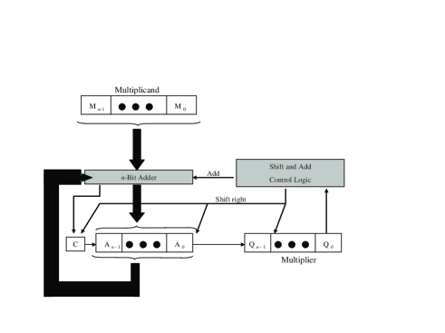
Figure 2: Classical multiplier architecture

Therefore, we encode the binary alphabet $\{1,0\}$ in another one, $\{0,1,-1\}$, that shows the transitions among the binary logic states within a binary chain. Thus, when a $-1$ is faced a subtraction and a shift are performed (using the 2’s-complement representation) and when a $1$ is faced an addition and a shift are performed. In the other two cases just an arithmetic shift is performed for each situation. The algorithm conforms to this scheme by performing a substraction when the first 1 of the block is encountered ($1\to 0$) and an addition when the end of the block is encountered ($0\to 1$). It is straightforward to show that the same scheme works for a negative multiplier using the 2’s-complement notation. The architecture of Booth’s algorithm is shown in Fig. 2, and an example for the multiplication of 7 (0111) by 3 (0011), is shown in Fig. 3. The multiplier and the multiplicand are placed in the $Q$ and $M$ registers, respectively. There is also a 1-bit register placed logically to the right of the less significant bit ($Q_{0}$) of the $Q$ register and designated $Q_{-1}$. The results of the multiplication will appear in the $A$ and $Q$ registers, the first one initialized to 0.

$$\boxed{\begin{array}[]{ccccl}A&Q&Q_{-1}&M\\ 0000&0011&0&0111&{\rm Initial\ Values}\\[12.91663pt] \begin{array}[]{c}1001\\ 1100\end{array}&\begin{array}[]{c}0011\\ 1001\end{array}&\begin{array}[]{c}0\\ 1\end{array}&\begin{array}[]{c}0111\\ 0111\end{array}&\left.\begin{array}[]{l}A\quad A-M\\ {\rm Shift}\end{array}\right\}\begin{array}[]{l}{\rm First}\\ {\rm Cycle}\end{array}\\[12.91663pt] \begin{array}[]{c}1110\end{array}&\begin{array}[]{c}0100\end{array}&\begin{array}[]{c}1\end{array}&\begin{array}[]{c}0111\end{array}&\left.\begin{array}[]{l}{\rm Shift}\phantom{xxxxx}\end{array}\right\}\begin{array}[]{l}{\rm Second}\\ {\rm Cycle}\end{array}\\[12.91663pt] \begin{array}[]{c}0101\\ 0010\end{array}&\begin{array}[]{c}0100\\ 1010\end{array}&\begin{array}[]{c}1\\ 0\end{array}&\begin{array}[]{c}0111\\ 0111\end{array}&\left.\begin{array}[]{l}A\quad A+M\\ {\rm Shift}\end{array}\right\}\begin{array}[]{l}{\rm Third}\\ {\rm Cycle}\end{array}\\[12.91663pt] \begin{array}[]{c}0001\end{array}&\begin{array}[]{c}0101\end{array}&\begin{array}[]{c}0\end{array}&\begin{array}[]{c}0111\end{array}&\left.\begin{array}[]{l}{\rm Shift}\phantom{xxxxx}\end{array}\right\}\begin{array}[]{l}{\rm Fourth}\\ {\rm Cycle}\end{array}\end{array}}$$

Figure 3: Example of Booth’s algorithm.

Control logic scans the bits of $Q_{0}$ and $Q_{-1}$ one at a time. According to Fig. 4,

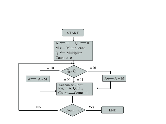
Figure 4: Flow chart for classical Booth’s algorithm.

if the two bits are the same, then all the bits of $A$, $Q$, and $Q_{-1}$ are shifted to the right one bit. If the two bits differ, then the multiplicand is added or subtracted from the $A$ register, according as the two bits are $(0\to 1)$ or $(1\to 0)$. Following the addition or subtraction, the right shift occurs. In either case, the right shift is such that the leftmost bit of $A$, namely $A_{n-1}$, not only is shifted into $A_{n-2}$, but also remains in $A_{n-1}$. This is required to preserve the sign of the number in $A$ and $Q$ and it is named arithmetic shift, since it preserves the sign bit.

II Quantum Booth Multiplier

In this section a QBM is presented. First of all, we have to encode the computational basis states $\{|0\rangle,|1\rangle\}$ that generate the Hilbert’s space $\mathcal{H}^{2}$ by the new alphabet $\{0,1,-1\}$ that will be represented by three orthonormal quantum states belonging to the computational basis that generates $\mathcal{H}^{2}\bigotimes\mathcal{H}^{2}$. These three states are $|00\rangle\,\equiv\,0$, $|01\rangle\,\equiv\,1$, $|10\rangle\,\equiv\,-1$, and have been chosen in this way because they form a Gray code of three elements: all of them just differ from each other in one binary digit. This will be a useful property that will simplify the control stage in the QBM architecture. Thus, the encoder, transforms the states couple $\left|{x_{i+1}}\right\rangle_{1}$$\left|{x_{i}}\right\rangle_{3}$ in its transformed $\left|{x^{\prime}_{i+1,i}}\right\rangle_{2}$$\left|{x^{\prime\prime}_{i+1,i}}\right\rangle_{3}$ by means of the table given in Fig. 5, representing the quantum operations performed by the quantum circuit that appears in Fig. 6.

Figure 5: Transforming the state of two adjacent qubits.

Figure 6: Booth’s encoding of two adjacent qubits.

If we would like to encode a 4-qubits binary chain, for instance, we should built the Booth Encoder circuit ($\mathcal{BE}$) shown in Fig. 7 and, for reversibility purposes, apply its inverse ($\mathcal{BE}^{-1}$), which is the same circuit but using the outputs as inputs, and viceversa

Figure 7: 4-qubits Quantum Booth Encoder.

Now, for our 4-qubits example, the QBM architecture can be described as follows. The quantum circuit shown in Fig. 7 encodes the binary transitions ($i+1,i$) and controls, by Toffoli gates, what will be stored at the quantum registers, where the partial products have been loaded. Hence, depending on the transitions in the quantum binary chain, we will perform one out of the three following operations over the multiplicand:

• If we have no transition, $|00\rangle$, then load 0’s in the partial product register.

• If we have up-transitions, $|01\rangle$, then load the multiplicand in the partial product register.

• If we have down-transitons, $|10\rangle$, then load the multiplicand 1’s-complement representation in the partial product register.

Finally, we have to sum all the partial products that we have generated. If the multiplicand and the multiplier have $n$ qubits, each partial product will have $2n$ qubits and they will be shifted, from the encoded multiplier Less Significant Bit (LSB) to the Most Significant Bit (MSB), depending on the ordinal position of the multipliers bits. These displacements are implemented within the quantum $2n$-registers hardware.

After the $\cal{O}(\log$ n$)$ sums have been performed we still have to do something more because we have used 1’s-complement representation instead of 2’s-complement representation. Indeed, we have saved the “carry” bit bearing in mind that 2’s-complement representation is equal to 1’s-complement representation plus one. Therefore, we have to add, to the whole partial products sum, another register where the 1’s have been stored in their ordinal proper way, as one can see in the example displayed in Fig. 8. Therefore, the final output is the desired input product represented in 2’s-complement.

III Conclusions

In this work a new Quantum Booth Algorithm is presented. Note that QBM has a very regular structure. It can be easily implemented in order to build bigger circuits for bigger inputs than the one shown in Fig. 8. Its delay is $\cal{O}((\log$ n$)^{2})$ due to the adders structure are $\cal{O}(\log$ n$)$ and each adder has a logarithmic deph. One could reduces it by means of a CSA scheme Sunar but it would made to lose the circuit regular structure, which is an undesireble compensation. Thus, the bottleneck are the adders and our future researching efforts will go in the direction of clarifying whether $\cal{O}(\log$ n$)$ is a fundamental bound, from the quantum physics point of view, or not. Note that adders information processing logarithmic-carry-add is classical due to that the input information is classical; there is nor entanglement neither quantum superposition. Therefore, the Quantum Booth Algorithm architecture is also a classical reversible one because the quantum gates used in the encoding and control stages are also classical reversible ones (TOFFOLI, SWAP, CNOT). No Hadamards are presented.

The main target of this paper was building a quantum algorithm for the multiplication task using the fundamental features that quantum computation has: entanglement and superposition of states. But, when we tried this way, we realized that we did not need quantum entanglement for building our quantum multiplying algorithm. The reason was that we were rewriting a classical irreversible algorithm by means of classical reversible gates (excluding Hadamard ones). Indeed, we believe that for obtaining a real improvement, it is necessary to reconsider the way in which the Quantum Arithmetic Logic Unit was designed, in order to perform the quantum arithmetic operations taking into account, as essential ingredients, quantum entanglement and quantum superposition. Work in this direction is in progress.

Figure 8: 4-qubits Quantum Booth’s array multiplier circuit

- (1) P. W. Shor (1997), Polynomial time algorithms for prime factorization and discrete logarithms on a quantum computer, SIAM J. Comput. 26 pp. 1484-1509 (quant-ph/9508027).
- (2) L. K. Grover (1997), Quantum computer can search arbitrarily large databases by a single querry, Phys. Rev. Lett. 79, pp. 4709-4712.
- (3) C.H. Bennett and G. Brassard (1984), Quantum Cryptography: public key distribution and coin tossing, Proc. of IEEE Int. Conf. on Computers Systems and Signal Porcessing, pp. 175-179.
- (4) V. Vedral, A. Barenco, and A. Ekert (1996), Quantum networks for elementary arithmetic operations, Phys. Rev. A 54, pp. 147-153 (quant-ph/9511018).
- (5) S. A. Cuccaro, T. G. Draper, S. A. Kutin and D. P. Moulton (2004), A new quantum ripple-carry addition circuit, quant-ph/0410184.
- (6) T. G. Draper, S. A. Kutin, E. M. Rains, and K. M. Svore (2004), A logarithmic-deph quantum carry-lookahead adder, quant-ph/ 0410184.
- (7) T. G. Draper (2000), Addition on a quantum computer, quant-ph/ 0008033.
- (8) W. Stallings (1996), Computer Organization and Architecture, Prentice-Hall. Inc.(New York).
- (9) M. M. Mano (1979), Digital logic and computer design, Prentice-Hall, Inc. (New York).
- (10) B. Sunar (2006), Computer Arithmetic Circuits, http:// ece.wpi.edu/ sunar/courses/ee579v/.