Geometric phase of an atom in a magnetic storage ring

Abstract

A magnetically trapped atom experiences an adiabatic geometric (Berry’s) phase due to changing field direction. We investigate theoretically such an Aharonov-Bohm-like geometric phase for atoms adiabatically moving inside a storage ring as demonstrated in several recent experiments. Our result shows that this phase shift is easily observable in a closed loop interference experiment, and thus the shift has to be accounted for in the proposed inertial sensing applications. The spread in phase shift due to the atom transverse distribution is quantified through numerical simulations.

I Introduction

A recent highlight in atom optics atomic optics is the realization of atomic storage rings Chapman ; Kurn1 ; Arnold3 ; Arnold2 ; Arnold4 . With well-designed magnetic (B-) field configurations, cold atoms including Bose-Einstein condensates can be confined in a ring shaped region with a diameter of the order of a mm Kurn1 , a cm Chapman , or 10 cm Arnold3 ; Arnold2 ; Arnold4 . Such a trapping geometry provides exciting prospects for delivering atoms into high Q optical cavities Chapman and for inertial sensing applications Arnold2 ; Sagnac .

Magnetic ring shape traps are formed by inhomogeneous magnetic fields. Accompanied by the trapped center of mass motion, the atomic spin adiabatically follows its local B-field direction, giving rise to a geometric (Berry’s) phase berry ; jorg ; Ho-Shenoy . This induces a phase shift in storage ring based interference, reminiscent of the Aharonov-Bohm effect from the magnetic gauge potential in electron interference. Even when confined in transverse motional ground state, a distribution of this geometric phase arises corresponding to atomic guiding trajectories at different transverse radii, potentially causing degradation to the interference contrast. Therefore a detailed investigation is essential for applications of ring based interferometry to high precision measurements.

The geometric phase of an atom in the widely used Ioffe-Pritchard trap was first studied in Ref. Ho-Shenoy , where the associated gauge potential (Berry’s connection) was also discussed for a general magnetic trap. The aim of this paper is a detailed investigation of this geometric phase for an atom in a magnetic storage ring. We find that it is simply related to the cosine value of the angle between the local B-field and the symmetry axis of the ring, a result easily understood in terms of the solid angle sustained by the adiabatic changing B-field along the central azimuthal closed trajectory of a storage ring. We have performed extensive numerical studies of the geometric phase as a function of the various components forming the trap field and elucidated the condition when the fluctuation of this geometric phase is small.

This paper is organized as follows: in Sec. II, we briefly review the atomic storage ring system and discuss the associated geometric phase. Based on the assumption of a simple classical center of mass motion of the atom, the geometric phase and the spatial fluctuation are calculated in Sec. III for various types of magnetic storage rings. In Sec. IV, we provide an full quantum treatment of this geometric phase in a hypothetical storage ring based interference experiment. Finally we conclude in Sec. V.

II Geometric phase in a storage ring

As in recent experiments Chapman ; Kurn1 ; Arnold3 ; Arnold2 ; Arnold4 , a magnetic storage ring can be formed by several axially-displaced concentric current carrying coils. Near the origin, the trap field takes the form $\vec{B}=B_{\rho}\hat{e}_{\rho}+B_{z}\hat{e}_{z}$ Arnold1 ; bergman with

$$B_{\rho} = -\frac{B_{1}}{2}\rho-\frac{B_{2}}{2}\rho z,$$

$$B_{z} = B_{0}+B_{1}z+\frac{B_{2}}{2}(z^{2}-\frac{\rho^{2}}{2}),$$ (1)

up to polynomial terms second order in the cylindrical coordinate $(\rho,\phi,z)$. The $B_{1}$ terms clearly resemble the quadruple B-field from a pair of anti-Helmholtz coils, while the $B_{0}$ and $B_{2}$ terms take the familiar expansions for a Ioffe-Pritchard trap Pritchard . It is easy to verify that when $B_{0}B_{2}>0$, the trap field vanishes at the point $\rho_{0}\hat{e}_{\rho}+z_{0}\hat{e}_{z}$ Arnold1 of

$$\rho_{0}=\sqrt{4B_{0}/B_{2}-2B_{1}^{2}/B_{2}^{2}},\ \ \ z_{0}=-B_{1}/B_{2}.$$ (2)

To avoid spin flipping (Majorana transition) near this zero B-field region, an azimuthal bias field Arnold2 can be added, or a time averaged potential can be constructed by rapidly oscillating the trap field $\vec{B}$ Arnold1 ; Kurn1 . In this paper we mainly focus on the more complicated case of a time averaged trap (TORT) from the recent experiment Kurn1 . When $B_{0,1,2}$ are oscillating functions of time with a large frequency $\omega$, the atomic motion will be governed by a time averaged potential $\propto(\omega/2\pi)\int_{0}^{2\pi/\omega}|\vec{B}(\vec{r},t)|dt$, provided adiabaticity is maintained. This requires $\omega$ to be much less than the atomic Larmor frequency in the trap field such that its spin remains aligned. Also $\omega$ has to be much larger than the time averaged trap frequency in order to make the trapping effective.

For simplicity, we will suppress the $(\rho,z)$ degrees of freedom and consider atomic motion parameterized by $\phi$ along the azimuthal $\hat{e}_{\phi}$ direction of the storage ring. Then the state of the atomic mass center would be described by the function $\phi(t)$. The interaction between an atom and the presumably weak trap field $\vec{B}[\phi,t]$ is governed by the linear Zeeman effect

$$H[\phi,t]=\mu_{\rm B}g_{F}\vec{F}\cdot\vec{B}[\phi,t],$$ (3)

where $\mu_{\rm B}$ is the Bohr magneton, and $\vec{F}$ is the atomic hyperfine spin. The Lande factor for the spin-1 manifold of a ⁸⁷Rb atom is $g_{F}=-1/2$. For simplicity we take $\hbar=1$. The trapped atomic spin is adiabatically aligned with respect to the local B-field, i.e., the atomic spin remains in the low field seeking internal state $|(-1)[\phi,t]\rangle_{B}$ of the instantaneous eigenstate of $H$ with eigenvalue $\epsilon_{-1}[t]=-\mu_{\rm B}g_{F}|\vec{B}|$. It is related to the eigenstate $|(-1)\rangle_{z}$ of $F_{z}$ (of eigenvalue $-1$) by a simple rotation

$$|(-1)[\phi,t]\rangle_{B}=\exp[-i\vec{F}\cdot\hat{e}_{\phi}\beta(t)]|(-1)\rangle_{z},$$ (4)

where $\beta(t)$ is the angle between $\vec{B}[\phi,t]$ and the $z$-axis. It is independent of $\phi$ due to the cylindrical symmetry.

In this section and the following section III, we treat the atomic center of mass motion is classically, by its one dimensional azimuthal angle $\phi(t)$ along the circumference of the ring (at fixed $\rho=\rho_{c}$ and $z=z_{c}$). The quantum treatment of the atomic center of mass motion will be given in section IV. According to the quantum adiabatic theorem adiabatic , an atom initially described by state $|\Psi(0)\rangle=|(-1)[\phi(0),0]\rangle_{B}$ becomes

$$|\Psi(t)\rangle=|(-1)[\phi(t),t]\rangle_{B}e^{-i\gamma_{d}(t)}e^{-i\gamma_{g}(t)},$$ (5)

at time $t$. $\gamma_{d}=\int_{0}^{t}\epsilon_{-1}[t^{\prime}]dt^{\prime}$ is the dynamical phase, and $\gamma_{g}(t)$ is the geometric phase, i.e., the Berry’s phase berry that is expressed as

$$\gamma_{g}(t) = -i\int_{0}^{t}\,{}_{B}\langle(-1)[\phi(t^{\prime}),t^{\prime}]|\frac{d}{dt^{\prime}}|(-1)[\phi(t^{\prime}),t^{\prime}]\rangle_{B}dt^{\prime}$$ (6)

$$= \int_{0}^{t}\cos[\beta(t^{\prime})]\Omega(t^{\prime})dt^{\prime},$$

with $\Omega(t)=d\phi/dt$ the atomic angular velocity along the storage ring. To obtain the above formula we used $d/dt=\partial_{t}+(d\phi/dt)\partial_{\phi}$ as well as the equalities $\,{}_{B}\langle(-1)[\phi,t]|\partial_{\phi}|(-1)[\phi,t]\rangle_{B}=i\cos\beta$ and $\,{}_{B}\langle(-1)[\phi,t]|\partial_{t}|(-1)[\phi,t]\rangle_{B}=0$ that come directly from our definition of $|(-1)[\phi,t]\rangle_{B}$ in Eq. (4).

The periodic time dependence of $\vec{B}[\phi,t]$ gives rise to the Fourier expansion $\cos[\beta(t)]=\cos\beta_{0}+\sum_{n>0}C_{n}\cos[n\omega t+\varphi_{n}]$ with $\cos\beta_{0}$ denoting the time averaged value of $\cos[\beta(t)]$. On substituting into Eq. (6), we find $\gamma_{g}=\cos\beta_{0}[\phi(t)-\phi(0)]+\sum_{n>0}C_{n}\int\cos[n\omega t^{\prime}+\varphi_{n}]\Omega(t^{\prime})dt^{\prime}$. The integral $C_{n}\int\cos[n\omega t^{\prime}+\varphi_{n}]\Omega(t^{\prime})dt^{\prime}$ takes the maximum value $2C_{n}\Omega/(n\omega)$ for a slowly varying function $\Omega(t)$, which becomes negligible when $\Omega$ is much smaller than $\omega$. In this case, we find the geometric phase $\gamma_{g}$ can be approximated as $\gamma_{g}(t)\approx\cos\beta_{0}[\phi(t)-\phi(0)]$, which is independent of $\Omega(t)$ and completely determined by the trajectory of the atom in the storage ring. For a closed path, we arrive at the geometric phase

$$\gamma_{C}=2\pi q\cos\beta_{0},$$ (7)

where $q$ is the familiar integer winding number of the atomic trajectory. More specifically, we find

$$\cos\beta_{0}=\frac{\omega}{2\pi}\int_{0}^{2\pi/\omega}\frac{B_{z}({\vec{r}}_{c},t)}{|\vec{B}({\vec{r}}_{c},t)|}dt,$$ (8)

within our approximation for various trap field configurations. In the above, ${\vec{r}}_{c}=\rho_{c}\hat{e}_{\rho}+z_{c}\hat{e}_{z}$ denotes the center position of the time averaged storage ring trap.

III Results

In the previous section, the general expression for the geometric phase (7) is obtained for an atom in a storage ring. This section is devoted to a study of the size and distribution of this phase for various types of magnetic storage ring. For a static storage ring trap formed by supplementing an azimuthal bias B-field from a current carrying wire along the symmetric axis as in Ref. Arnold2 , the Berry’s phase vanishes because $\beta_{0}\equiv\pi/2$. For a TORT trap, the dependence of $\cos\beta_{0}$ on the trap parameters $B_{0,1,2}$ of Eq. (1) can be investigated. When $B_{2}$ is a constant, $\cos\beta_{0}$ is closely related to the oscillation amplitude of $B_{1}$. For the following simple time dependence

$$B_{0}=B_{2}[L^{2}+n^{2}\sin(\omega t)],\ \ B_{1}=B_{2}l\cos(\omega t),$$ (9)

parameterized by length scales $L$, $n$, and $l$, we find that the value of $\cos\beta_{0}$ is mainly determined by $l/L$. In Fig. 1(a), the $l/L$ dependence of $\cos\beta_{0}$ is shown for different values of $n/L$. We see that $\cos\beta_{0}$ behaves as an increasing function of $l/L$. For $n=0$, it turns into an approximate linear dependence $\cos\beta_{0}=0.3l/L$. In Fig. 1(b), the storage ring trap center $\rho_{c}$ is shown for $n=0$. It behaves like a quadratically decreasing function of $l/L$.

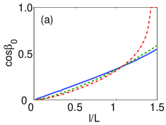
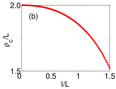
Figure 1: (Color online) (a) The dependence of $\cos\beta_{0}$ on $l/L$ for $n=0$ (solid line), $n=3L/4$ (dashed line), and $n=L$ (dash-dot line). (b) The dependence of $\rho_{c}/L$ on $l/L$ for $n=0$.

During oscillation, the zero field point of Eq. (2) traces out a closed trajectory in the cross section of the storage ring. In the proposal of Ref. Arnold1 and the experiment Kurn1 , this closed trajectory forms a loop (a torus in 3D) surrounding the center ($\rho_{c},z_{c}$) along the storage ring. For a constant $B_{2}$, the oscillation amplitude of $B_{1}$ is proportional to the radius of this “death torus” Kurn1 in the $z$-direction. If the radius becomes sufficiently small, e.g., as in Fig. 3(b) of Ref. Arnold1 , the value of $\cos\beta_{0}$ in the trap center also becomes very small. The locus of the zero point for our example is plotted in Fig. 2(a). The trajectory that forms the boundary of the loop (torus) has now collapsed into an open curve on one side of the trap center, although the time averaged trap potential is still well established as illustrated in Fig. 2(b). We have also calculated the Fourier coefficients $C_{n}$ of $\cos\beta(t)$. In Fig. 3(a), the two largest coefficients $C_{2}$ and $C_{4}$ are plotted as functions of $l/L$. We note that their maximum values remain much smaller than unity.

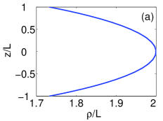
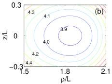
Figure 2: (Color online) (a) The locus of the zero field point for the trap’s B-field. (b) The equal B-field contours of the time averaged magnetic field. The B-field is in units of $B_{0}$. Both figures are for $n=0$ and $l=L$.

In the above calculation, the classical center of mass motion of the trapped atom along the storage ring is at a fixed ${\vec{r}}_{c}$. In reality, the atomic center of mass position $(\rho,z)$ may deviate from $(\rho_{c},z_{c})$ even for a closed trajectory. This uncertainty of atomic position in the cross sectional plane can be due to either transverse atomic thermal motion or the quantum nature of the transverse motional state. In the following calculation for the fluctuations, we consider the simple case of a transverse distribution reflected for instance by its motional ground state. This then leads to a genuine dependence of the geometric phase on the values of transverse coordinates $\rho$ and $z$. This causes fluctuations of the phase shift, which can lower interference contrast or even destroy interference fringes from the atomic wave packet in the $\phi$ direction as we discuss in next section. Within the semi-classical framework we adopt, the fluctuations can be approximately simulated by a probabilistic sampling of the values for $\rho$ and $z$ as reflected by their probability distributions in the transverse motional ground state. To arrive at a high contrast interference pattern, the spread of this phase fluctuation should be kept small. We have calculated the variations of this fluctuation with respect to different parameters of a TORT trap. In Fig. 3(b), the fluctuation defined according to $f=\sqrt{\langle[\cos\beta_{0}(\vec{r})-\cos\beta_{0}(\vec{r}_{c})]^{2}\rangle}$ is plotted as a function of $l/L$ for $\delta=0.001L$, $\delta=0.005L$ and $\delta=0.015L$. Here $\cos\beta_{0}(\vec{r})$ is the time averaged value of $B_{z}/|B|$ at the position $\vec{r}=\rho\hat{e}_{\rho}+z\hat{e}_{z}$. The average $\langle\cdot\rangle$ is over a properly weighted, assumed here for simplicity as a flat spatial distribution in the region $R:\{\rho\in[\rho_{c}-\delta,\rho_{c}+\delta],z\in[z_{c}-\delta,z_{c}+\delta]\}$. $f$ is found to be a decreasing function of $l/L$. Together with Fig. 1(a), we conclude that when $l/L$ is large, the value of $\cos\beta_{0}$ is also large with small fluctuations.

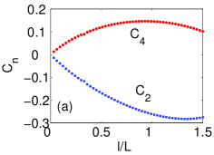
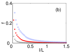
Figure 3: (Color online) (a) The $l/L$ dependence of $C_{2}$ ($C_{4}$) in blue (red) squares. (b) The fluctuation of $\cos\beta_{0}$ over the region $\delta=0.015L$ (blue empty square), $\delta=0.005L$ (red circle) and $\delta=0.001L$ (black plus sign).

Finally we illustrate a practical example for $B_{2}=7800$ Gauss$\cdot$cm^-2 and $L=l=n=0.1$ cm. The bias field $B_{0}(t)$ is $78[1+\sin(\omega t)]$ Gauss and the first order B-field gradient $B_{1}(t)$ becomes $780\sin(\omega t)$ Gauss$\cdot$cm^-1. In this case the trap frequencies in the $\rho$- and $z$- directions are $345$Hz and $672$Hz, respectively. The time averaged Berry’s phase is $2\pi\cos\beta_{0}\approx 0.2\pi$. This trap can be realized with two pairs of Helmholtz coils (a and b) centered at $(z=\pm A_{a,b},\rho=0)$ and a pair of anti-Helmholtz coils c centered at $(z=\pm A_{c},\rho=0)$ with $A_{a}=0.1$cm, $A_{b}=0.25$cm, and $A_{c}=0.5$cm, respectively. The radii $R_{a,b,c}$ of the three pairs of coils are taken as $R_{a}=0.3$cm, $R_{b}=0.5$cm, and $R_{c}=0.6$cm with currents in the two Helmholtz pairs being $i_{a}=289$A and $i_{b}=-550$A, and in the anti-Helmholtz coils are $i_{c}=335$A.

IV The Aharonov-Bohm like phase shift from a quantum treatment

The geometric phase as discussed above is directly measurable, e.g., in the Sagnac interferometer Sagnac . For this purpose, we perform a calculation capable of a quantum treatment of atomic motion. Trapped atoms are assumed to be in the guiding regime so that their transverse degrees of freedom, $\rho$ and $z$, are frozen in the ground state. Writing the atomic wave function as $\Phi(\phi,t)|(-1)(\phi,t)\rangle_{B}$ with $\Phi(\phi,t)$ for its spatial motion, we find that the Schrodinger equation $i(d/dt)\Psi=H_{\rm ad}\Psi$ is governed by a time averaged adiabatic Hamiltonian sunandother

$$H_{\rm ad}=\frac{1}{2m}{\left[p_{\phi}-{A(\phi)}/{\rho_{c}}\right]^{2}}+V(\phi).$$ (10)

$V(\phi)$ denotes the time averaged trap potential that more generally can contain additional optical or the gravitational potentials. $A(\phi)=-i(\omega/2\pi)\int_{0}^{2\pi/\omega}\ {}_{B}\langle(-1)(\phi,t)|\partial_{\phi}|(-1)(\phi,t)\rangle_{B}dt$ is the time averaged gauge potential. For the simple case considered previously, $A$ equals $\cos\beta_{0}$ and is independent of $\phi$. In this section, without loss of generality, we assume $A(\phi)$ to be a slowly varying function of $\phi$. The operator $p_{\phi}=-i\rho_{c}^{-1}\partial/\partial_{\phi}$ denotes the atomic canonical momentum along the $\hat{e}_{\phi}$ direction. In the presence of the gauge potential $A(\phi)$, the atomic kinetic angular velocity $v_{\phi}$ becomes $v_{\phi}=p_{\phi}/(m\rho_{c})-A(\phi)/(m\rho_{c}^{2})$.

We note that the Hamiltonian in Eq. (10) only applies when the gauge potential $A$ do not depend strongly on $\rho$ and $z$, as otherwise their dependence in the term $A(\phi,\rho,z)p_{\phi}$ would lead to inseparable correlations between the dependencies on $\phi$, $\rho$, and $z$ of the atomic wave function. If this does occur, the reduced atomic quantum state for the $\phi$ direction becomes a mixed state rather than a pure one, resulting in reduced coherence property. This constitutes a quantum explanation for the reduced contrast in the interference pattern due to fluctuations of the geometric phase.

Obviously this Hamiltonian (10) resembles the motion of an electron around a current carrying solenoid, where an Aharonov-Bohm (A-B) phase AB effect is induced by the corresponding vector potential, with a value proportional to its integral along a closed path surrounding the solenoid. In our case, we expect essentially the same result with an Aharonov-Bohm-like phase, or the Berry’s phase $\gamma_{C}$ as defined in Eq. (7), given by the line integral of the induced gauge potential $\int A(\phi)d\phi$. In the A-B effect of an electron, both the electron source and the detector (screen) are far away from the solenoid, where the vector gauge potential vanishes. The electron achieves a steady asymptotic distribution long before and after ($t\to\pm\infty$) the encounter with the solenoid. Therefore its motion can be treated via stationary scattering theory AB effect ; ABBerry or based on a path integral approach with an incident plane wave cohen . For our case of trapped atoms in a storage ring, the gauge potential $A(\phi)$ never vanishes at any instant during the evolution. Thus our model must be treated dynamically as described by a time dependent Schrodinger equation.

We first consider the motion of a single wave packet assuming that $A(\phi)$ varies slowly and is approximated as a constant in the region, where the wave function is non-negligible. The expectation value of the atomic position $\phi$, the canonical momentum $p_{\phi}$, and the velocity $v_{\phi}$ of the wave packet at time $t$ will be denoted as $\bar{\phi}_{t}$, $\bar{p}_{t}$, and $\bar{v}_{t}$. At $t=0$ the wave packet $\varphi(\phi,0)$ can be written as

$$\varphi(\phi,0)=\psi(\phi,0)e^{iA(\bar{\phi}_{0})(\phi-\bar{\phi}_{0})}.$$ (11)

Both $\bar{\phi}_{0}$ and $\bar{v}_{0}$ are determined completely through $\psi(\phi,0)$,

$$\bar{\phi}_{0} = \int\phi|\psi(\phi,0)|^{2}d\phi,$$

$$\bar{v}_{0} = -i{1\over{m\rho_{c}}}\int\psi^{*}(\phi,0)\partial_{\phi}\psi(\phi,0)d\phi,$$ (12)

independent of the gauge function $A$.

The Hamiltonian $H_{\rm ad}$ (10) can be obtained from the one without gauge potential $A(\phi)$ via a transformation, i.e., $H_{\rm ad}=UH_{0}U^{-1}$ with

$$H_{0}=\frac{p_{\phi}^{2}}{2m}+V(\phi),\ U=\exp[i\int_{\bar{\phi}_{0}}^{\phi}A(\phi^{\prime})d\phi^{\prime}],$$ (13)

provided the wave packet is limited to and moving in a finite region over the circumference. Therefore, $\varphi(\phi,t)$ is written as

$$\varphi(\phi,t) \approx \psi(\phi,t)e^{iA(\bar{\phi}_{t})(\phi-\bar{\phi}_{t})}e^{i\int_{\bar{\phi}_{0}}^{\bar{\phi}_{t}}A(\phi^{\prime})d\phi^{\prime}},$$ (14)

with $\psi(\phi,t)=e^{-iH_{0}t}\psi(\phi,0)$, where we have used the relation $e^{-iHt}=Ue^{-iH_{0}t}U^{-1}$ and replaced $A(\phi)$ with $A(\bar{\phi}_{0})$ [$A(\bar{\phi}_{t})$] in the region where $\psi(\phi,0)$ [$\psi(\phi,t)$] is non-negligible. The center position (velocity) $\bar{\phi}_{t}$ ($\bar{v}_{t}$) of each wave packet and the variation of the profile $\psi$ are also determined by $H_{0}$ independent of $A(\phi)$.

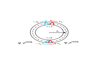
Figure 4: (Color online) A proposed setup of interferes in a storage ring. An initial superposition of two wave packets $\psi_{\pm}(\phi)e^{iA(0)\phi}$ with counter propagating velocities $\pm v_{0}$ interferences at time $T$ when the packets overlap near the other end $\bar{\phi}^{(+)}_{T}$.

To detect the geometric phase, we consider an interference set up as shown in Fig. 4 with the initial atomic state being a superposition of two counter propagating wave packets $\psi_{\pm}e^{iA(0)\phi}$ centered at $\phi=0$

$$\Phi(\phi,0)=\frac{1}{\sqrt{2}}\left[\psi_{+}(\phi,0)e^{iA(0)\phi}+\psi_{-}(\phi,0)e^{iA(0)\phi}\right].$$ (15)

The two wave packets overlap again at time $T$ when $\bar{\phi}^{(+)}_{T}=\bar{\phi}^{(-)}_{T}+2\pi$. Making use of Eq. (14), we find

$$\Phi(\phi,T)=\frac{1}{\sqrt{2}}[\psi_{+}(\phi,T)e^{iA(\bar{\phi}^{(+)}_{T})(\phi-\bar{\phi}^{(+)}_{T})}e^{i\int_{0}^{\bar{\phi}^{(+)}_{T}}A(\phi^{\prime})d\phi^{\prime}}$$

$$+\psi_{-}(\phi-2\pi,T)e^{iA(\bar{\phi}^{(+)}_{T})(\phi-\bar{\phi}^{(+)}_{T})}e^{i\int_{0}^{\bar{\phi}^{(+)}_{T}-2\pi}A(\phi^{\prime})d\phi^{\prime}}],$$ (16)

with $\psi_{\pm}(\phi,T)=e^{-iH_{0}T}\psi_{\pm}(\phi,0)$. A substitution of $\phi\rightarrow\phi-2\pi$ to the counter propagating wave packet defines the complete wave function over the same azimuthal region $(0,2\pi)$. An interference pattern $\propto\cos[\eta_{+}(\phi)-\eta_{-}(\phi)+\gamma_{C}]$ then reveals the presence of the phase shift $\gamma_{C}$, where $\eta_{+}$ ($\eta_{-}$) is defined as the phase of $\psi_{+}(\phi,T)$ [$\psi_{-}(\phi-2\pi,T)$]. Since the evolution of $\psi_{\pm}$ is governed by $H_{0}$, the density distribution $n_{\pm}(\phi)$ for each component and the phase difference $\eta_{+}(\phi)-\eta_{-}(\phi)$ are independent of $A(\phi)$. The induced gauge potential causes a shift, simply the geometric phase shift $\gamma_{C}$, to the interference pattern.

In many situations, the center of mass motion for the two interfering paths of an atom can be described classically. In this case the interference pattern can be predicted with more detail. We show in the appendix that Eq. (14), which describes the motion of a single wave packet, can be generalized to the following

$$\varphi(\phi,t)\approx e^{iS_{\rm cl}[\bar{\phi}_{t},t;\bar{\phi}_{0},0]}e^{i[\bar{p}_{t}-\bar{p}_{0}][\phi-\bar{\phi}_{t}]}e^{-i[\bar{\phi}_{t}-\bar{\phi}_{0}]p_{\phi}}\varphi(\phi,0),$$

(17)

with $\bar{\phi}_{t}$ and $\bar{p}_{t}$ denoting the expectation values for the position and its canonical momentum that satisfy the Hamiltonian equation governed by $H_{\rm ad}$, i.e., the center velocity $\bar{v}_{t}$ of the wave packet satisfies

$$\bar{v}_{t}=\bar{p}_{t}-A(\bar{\phi}_{t})=d\bar{\phi}_{t}/dt.$$ (18)

As we have pointed out before, the classical trajectory $\bar{\phi}_{t}$ and the speed $\bar{v}_{t}$ are independent of the gauge potential $A(\phi)$ because the dynamics is one dimensional. The global phase $S_{\rm cl}$ is defined as the action function in classical mechanics:

$$S_{\rm cl}(\bar{\phi}_{t},t;\bar{\phi}_{0},0)=\int_{0}^{t}L[\bar{\phi}_{t^{\prime}},\bar{v}_{t^{\prime}}]dt^{\prime},$$ (19)

where $L[\bar{\phi}_{t},\bar{v}_{t}]=\bar{v}_{t}^{2}/2+A(\bar{\phi}_{t})\bar{v}_{t}-V(\bar{\phi}_{t})$ is the Lagrangian function in classical mechanics. With this semiclassical description for the wave packet inside the storage ring, we find that the relative phase $[\eta_{+}(\phi)-\eta_{-}(\phi)+\gamma_{C}]$ can be approximated more transparently as $[m\rho_{c}(\bar{v}^{(+)}_{T}-\bar{v}^{(-)}_{T})\phi+\xi+\gamma_{C}]$ with a gauge-independent constant

$$\xi = \eta_{0+}(0)-\eta_{0-}(0)+\int_{0}^{\bar{\phi}^{(+)}_{T}}[(\rho_{c}\bar{v}_{t}^{(+)})^{2}/2-V(\bar{\phi}^{(-)}_{t})]dt$$ (20)

$$-\int_{0}^{\bar{\phi}^{(-)}_{T}}[(\rho_{c}\bar{v}_{t}^{(-)})^{2}/2-V(\bar{\phi}^{(-)}_{t})]dt.$$

The discussions outlined in this section also allow for easy calculations of more general Aharonov-Bohm like phase shifts due to different gauge effects in storage ring based matter wave interference experiments. For example, the matter wave Sagnac effect, which can be considered as an analog of the Aharonov-Bohm effect sagnac-2 , is easily deduced to correspond to a phase shift $2\pi m\Omega\rho_{c}^{2}\cos\theta$ in a storage ring set up, with $\Omega$ being the angular velocity for rotation and $\theta$ being the angle between the axis of rotation and the $z$ direction. The deduction simply involves replacing the adiabatic gauge protectional $A(\phi,t)$ with $m\Omega\rho_{c}^{2}\cos\theta$, which is proportional to the $\phi$-component of the ”gauge field” $m\vec{\Omega}\times\vec{r}$ for the Sagnac effect sagnac-2 .

V Conclusion

In this paper, we have presented the theoretical analysis of the geometric phase for a neutral atom inside a magnetic storage ring. For the interesting example of a time averaged potential (TORT), we have shown that the geometric phase is proportional to the averaged cosine value of the angle between the local B-field and the $z$ axis. When the oscillation amplitude of the quadruple component $B_{1}$ is large, a significant and sharply peaked geometric phase is realized on completing a single pass along the storage ring. Of course the net effect is cumulative with respect to the number of turns an atom makes. We hope our result will shine new light on the proposed inertial sensing experiments based on trapped atoms in storage rings.

Appendix A The One Dimensional Semi-Classical Motion of a Single Wave Packet

During the course of this work, we obtained some interesting results on the semi-classical one-dimensional motion for an atomic wave packet. These are summarized here because to our knowledge, they do no seem to have been stated or known anywhere.

Essentially the following material provides a proof of Eq. (17) which describes the one dimensional semi-classical motion of a single wave packet $\varphi(\phi,t)$. Our calculation is based on the following two assumptions:

1. During the whole evolution, the wave packet is assumed to be sufficiently narrow that the potential $V(\phi)$ can be approximated by a linear function in $\phi$ and the gauge potential $A_{\phi}$ assumed a constant in the region where the wave packet is non-negligible;

2. The evolution time is so short that the effect of wave packet diffusion can be omitted.

With the first assumption, it is easy to prove cohen quantum that the center position $\bar{\phi}_{t}$, the center canonical momentum $\bar{\phi}_{t}$, and the center velocity $\bar{v}_{t}$ satisfy the classical Hamiltonian equations

$${d\bar{\phi}_{t}\over dt} = \bar{v}_{t}=\bar{p}_{t}-A(\bar{\phi}_{t}),$$

$${d\bar{p}_{t}\over dt} = -\frac{\partial}{\partial\bar{p}_{t}}H_{\rm ad}(\bar{\phi}_{t},\bar{p}_{t}).$$ (21)

As we have shown in Eq. (11), at $t=0$, the wave packet can be written as $\varphi(\phi,0)=\psi(\phi,0)e^{iA(\bar{\phi}_{0})(\phi-\bar{\phi}_{0})}$. Furthermore, we can express the profile $\psi(\phi,0)$ as

$$\psi(\phi,0)=\int dpf(p,0)e^{-ip(\phi-\bar{\phi}_{0})}e^{-i\bar{v}_{0}(\phi-\bar{\phi}_{0})},$$ (22)

where the function $f(p,0)$ describes the momentum distribution at $t=0$.

At time $t$, the atomic wave function $\varphi(\phi,t)$ is expressed as in Eq. (14), determined by $\psi(\phi,t)=e^{-iH_{0}t}\psi(\phi,0)$. To calculate the wave function $\psi(\phi,t)$, we first replace the trap potential $V(\phi)$ with a time dependent linear potential $V_{0}(t)+V_{1}(t)\phi$ with

$$V_{0}(t) = V(\bar{\phi}_{t})-\frac{dV(\phi)}{d\phi}\Big{|}_{\phi=\bar{\phi}_{t}}\bar{\phi}_{t},$$

$$V_{1}(t) = \frac{dV(\phi)}{d\phi}\Big{|}_{\phi=\bar{\phi}_{t}}.$$

The Hamiltonian equation (21) satisfied by the center position and velocity can now be casted in the form of a Newtonian equation

$$d^{2}\bar{\phi}_{t}/dt^{2} = -V_{1}(t),$$

$$d\bar{\phi}_{t}/dt = \bar{v}_{t},$$ (23)

which can be solved as

$$\bar{\phi}_{t} = \bar{\phi}_{0}+\bar{v}_{0}t-\int_{0}^{t}dt_{1}\int_{0}^{t_{1}}dt_{2}V_{1}(t_{2}),$$

$$\bar{v}_{t} = \bar{v}_{0}-\int_{0}^{t}dt_{1}V_{1}(t_{1}).$$ (24)

According to the first assumption, the wave function $\psi(\phi,t)=e^{-iH_{0}}\psi(\phi,0)$ satisfies the Schoredinger equation

$$i\partial_{t}\psi(\phi,t)=H_{\rm eff}(t)\psi(\phi,t),$$ (25)

approximately, with the effective Hamiltonian

$$H_{\rm eff}(t)=\frac{p_{\phi}^{2}}{2}+V_{0}(t)+V_{1}(t)\phi.$$ (26)

Because the effective Hamiltonian $H_{\rm eff}$ is a quadratic function, the Schrödinger Eq. (25) can be solved with the Wei-Norman algebra method wei-norman . After direct calculation, we find

$$\psi(\phi,t)={\cal U}(t)\psi(\phi,0),$$ (27)

with the evolution operator given by

$${\cal U}(t)=e^{-ia(t)p_{\phi}^{2}}e^{-ib(t)p_{\phi}}e^{-ic(t)\phi}e^{-id(t)},$$ (28)

parameterized by

$$\begin{array}[]{lll}a(t)&=&t/2,\\ b(t)&=&\int_{0}^{t}dt_{1}t_{1}V_{1}(t_{1}),\\ c(t)&=&\int_{0}^{t}dt_{1}V_{1}(t_{1}),\\ d(t)&=&\int_{0}^{t}dt_{1}V_{0}(t_{1})+\int_{0}^{t}dt_{1}\int_{0}^{t_{1}}dt_{2}V_{1}(t_{1})t_{2}V_{1}(t_{2}).\end{array}$$ (33)

In the end, we find

$$\psi(\phi,t)=e^{iS_{0}(t)}\int dpf(p,t)e^{-ip(\phi-\bar{\phi}_{t})}e^{-i\bar{v}_{t}(\phi-\bar{\phi}_{t})},\ \ \$$ (34)

with $f(p,t)=f(p,0)e^{-ip^{2}t/2}$ and the global phase factor

$$S_{0}(t)=\int_{0}^{t}L_{0}[\bar{\phi}_{t^{\prime}},\bar{v}_{t^{\prime}}]dt^{\prime},$$ (35)

with $L_{0}[\bar{\phi}_{t},\bar{v}_{t}]=\bar{v}_{t}^{2}/2-V_{0}(t)-V_{1}(t)\bar{\phi}_{t}$. In the above derivation, we have used Eq. (24) and the relationship $\int_{0}^{t}dt_{1}(t-t_{1})V_{1}(t_{1})=\int_{0}^{t}dt_{1}\int_{0}^{t_{1}}dt_{2}(t-t_{1})V_{1}(t_{2})$.

If $t$ is so small that the momentum uncertainty $\Delta p$ of the wave function $\psi(\phi,0)$ remains small, we can omit the wave packet diffusion and assume $f(p,t)\approx f(p,0)$, which is our second assumption above. With this approximation and substituting Eq. (34) into Eq. (14), we obtain Eq. (17). Of course, this same result can also be deduced with the method in Sec. 3 of Ref. sun .

References

- (1) C. S. Adams and E. Riis, Prog. Quantum Electron. 21, 1 (1997); E. A. Hinds and I. G. Hughes, J. Phys. D 32, R119 (1999).
- (2) S. Gupta, K. W. Murch, K. L. Moore, T. P. Purdy, and D. M. Stamper-Kurn, Phys. Rev. Lett. 95, 143201 (2005); K. W. Murch, K. L. Moore, S. Gupta, and D.M. Stamper-Kurn, Phys. Rev. Lett. 96, 013202 (2005).
- (3) J. A. Sauer, M. D. Barrett, and M. S. Chapman, Phys. Rev. Lett. 87, 270401 (2001).
- (4) A.S. Arnold and E. Riis, J. Mod. Opt. 49, 959 (2002).
- (5) C. S. Garvie, E. Riis, and A. S. Arnold, Laser Spectroscopy XVI, edited by P. Hannaford et al. (World Scientific, Singapore, 2004), p. 178, see also www.photonics.phys.strath.ac.uk.
- (6) A.S. Arnold, C.S. Garvie, and E. Riis, Phys. Rev. A 73, 041606(R) (2006).
- (7) M. G. Sagnac, C. R. Hebd. Seances Acad. Sci. 157, 708 (1913).
- (8) M. V. Berry, Proc. R. Soc. Lond. A 392, 45 (1984).
- (9) J. Schmiedmayer et al., p. 72, Atom interferometry, edited by P. Berman, (Academic Press, N.Y. 1997).
- (10) T. Ho and V. B. Shenoy, Phys. Rev. Lett. 77, 2595 (1996).
- (11) A. S. Arnold, J. Phys. B 37, L29 (2004).
- (12) T. Bergeman, G. Erez, and H. J. Metcalf, Phys. Rev. A 35, 1535 (1987).
- (13) D. E. Pritchard, Phys. Rev. Lett. 51, 1336 (1983).
- (14) M. Born and V. Fock, Zeit. F. Physik 51, 165 (1928); J. Kato, J. Phys. Soc. Jap. 5, 435 (1950); L. I. Schiff, Quantum Mechanics, 3rd ed., (McGraw-Hill, N.Y., 1968).
- (15) C. A. Mead and D. G. Truhlar, J. Chem. Phys. 70, 2284 (1979); C. A. Mead, Phys. Rev. Lett. 59, 161 (1987); C. P. Sun and M. L. Ge, Phys. Rev. D 41, 1349 (1990).
- (16) Y. Aharonov and D. Bohm, Phys. Rev. 115, 485 (1959).
- (17) M. V. Berry, Eur. J. Phys. 1, 240 (1980).
- (18) P. Storey and C. Cohen-Tannoudji, J. Phys. II 4, 1999 (1994).
- (19) B. H. W Hendricks et al., Quantum Opt. 2, 13 (1990).
- (20) C. Cohen-Tanoudji, B. Diu, and F. Lalo, Quantum Mechanics, (Hermann and John Wiley Sons Inc., Paris, 1977).
- (21) J. Wei and E. Norman, J. Math. Phys. 4A, 575 (1963); C.P. Sun and Q. Xiao, Commun. Theor. Phys. 16, 359 (1996).
- (22) C. P. Sun et al., Eur. Phys. J. D 13, 145 (2001).