Quantum information processing using strongly-dipolar coupled nuclear spins

Abstract

Dipolar coupled homonuclear spins present challenging, yet useful systems for quantum information processing. In such systems, eigenbasis of the system Hamiltonian is the appropriate computational basis and coherent control can be achieved by specially designed strongly modulating pulses. In this letter we describe the first experimental implementation of the quantum algorithm for numerical gradient estimation on the eigenbasis of a four spin system.

An important issue in experimental quantum information processing (QIP) is achieving coherent control while increasing the number of qubits divincenzo ; corychuangrev . In all existing implementations of quantum computation, the execution time is limited by durations of nonlocal gates. In the case of nuclear magnetic resonance (NMR) implementations of QIP, where qubits are formed by mutually coupled spin 1/2 nuclei, most of the existing implementations used isotropic liquids. In these systems, the durations of nonlocal gates are limited by the strength of (indirect) scalar couplings, which typically are of the order of 10-100 Hz.

Apart from the scalar couplings, nuclear spins also interact through magnetic dipole-dipole couplings, which are 2-3 orders of magnitude stronger than the scalar couplings, and would therefore allow significantly faster gate operations. In the case of isotropic liquids, the rapid molecular reorientation averages the dipolar interactions to zero. On the other hand, in oriented systems, the dipolar interactions survive and are therefore potentially better candidates for NMR-QIP cory3qss .

The Hamiltonian for a dipolar coupled $n$-spin system is,

$${\cal H}=\sum_{j=1}^{n}\hbar\omega_{j}I^{j}_{z}+\sum_{j=1,k<j}^{n}2\pi\hbar{\mathrm{D}}_{jk}(3{\mathrm{I}}_{z}^{j}\cdot{\mathrm{I}}_{z}^{k}-{\mathrm{\bf I}}^{j}\cdot{\mathrm{\bf I}}^{k})$$ (1)

where $\omega_{j}$ are the chemical shifts, ${\mathrm{D}}_{jk}$ are the dipolar coupling constants and $I_{z}^{j}$ are z-components of the spin angular momentum operators I^j ernstbook . The first term corresponds to the Zeeman interaction and the second term describes the dipolar interaction. When $|\mathrm{D}_{jk}|\ll|\omega_{j}-\omega_{k}|$, one usually invokes the ‘weak-coupling’ approximation ernstbook ; levittbook , where one ignores the off-diagonal parts of the Hamiltonian. Then the Zeeman product states are the eigenstates of the full Hamiltonian and individual spins can be conveniently treated as qubits. Most of the experiments in NMR-QIP have so far been carried out on such systems corychuangrev .

However to maximize the execution speed of our quantum processor it is desirable to use stronger couplings, including $|\mathrm{D}_{jk}|\geq|\omega_{j}-\omega_{k}|$. In this case, we have to use the complete Hamiltonian (1), where the Zeeman and the coupling parts do not commute and not all eigenstates are Zeeman product states but linear combinations of them. Unlike in the case of a weakly coupled spin system, individual spins of a strongly coupled system loose addressability. In such cases the eigenstates of the full Hamiltonian can form individually controllable subsystems and then the eigenbasis becomes the natural and accurate choice for the computational basis.

Though strongly dipolar coupled spin-systems have been suggested for QIP earlier maheshCS , so far it had not been possible to implement general unitary gate operations that can be applied to arbitrary initial conditions. Here we show how quantum computation can be realized on the eigenbasis by efficient coherent control techniques. As a specific system, we use a strongly dipolar coupled four-spin system partially oriented in a liquid crystal. Such systems have certain key merits. Unlike in the liquid state systems, the intramolecular dipolar couplings are not averaged out completely, but are only scaled down by the order parameter of the solute molecules oriented in the liquid crystal diehlvol6 ; emsleybook . Since intermolecular interactions are averaged out (unlike the crystalline systems), liquid crystalline systems provide well defined quantum registers with low decoherence rates. We achieve high-fidelity coherent control with the help of specially designed strongly modulating pulses (SMPs).

To demonstrate these techniques, we use an interesting algorithm suggested by S. P. Jordan spjordan : the quantum algorithm for numerical gradient estimation (QNGE). Before we discuss our implementation, we summarize the theoretical description of QNGE spjordan . The gradient of an one-dimensional real function $f$ over a small real range $l$ is written as $\nabla f=\{f(l/2)-f(-l/2)\}/l$. Thus classically two function evaluations are necessary to estimate the gradient of a one-dimensional function and a minimum of $d+1$ function evaluations are necessary for a $d$-dimensional function. On the other hand, QNGE requires only one function evaluation independent of the dimension of the function. Here the function $f$ is encoded in an $n$-qubit input register. An ancilla register is also required whose size ($n_{0}$ qubits) depends on the maximum possible value of the gradient.

In QIP, numbers are represented in binary form. To encode the real number $x$ in the input register, we have to convert it into a nonnegative integer $\delta\in\{0,1,\cdots,N-1\}$, where $N=2^{n}$. The encoding is defined by

$$x=\frac{l}{N-1}\left(\delta-\frac{N-1}{2}\right).$$ (2)

The circuit diagram for the quantum algorithm is shown in Figure 1.

Figure 1: Circuit diagram for QNGE.

Initially the ancilla register ($an$) is set to 1 and the input register ($in$) is set to 0. The inverse quantum Fourier transform (IQFT) prepares a plane wave state on the ancilla register and and the Hadamard transform (H) prepares a uniform superposition on the input register chuangbook :

$$\underbrace{|00\cdots 01\rangle}_{an}\underbrace{|00\cdots 00\rangle}_{in}\stackrel{{\scriptstyle\mathrm{IQFT}^{an}}}{{\longrightarrow}}\stackrel{{\scriptstyle\mathrm{H}^{in}}}{{\longrightarrow}}$$

$$\hskip 56.9055pt\frac{1}{\sqrt{N_{0}}}\sum_{k=0}^{N_{0}-1}e^{-i\frac{2\pi k}{N_{0}}}|k\rangle\frac{1}{\sqrt{N}}\sum_{\delta=0}^{N-1}|\delta\rangle$$

The ancilla register is now in an eigenstate of the addition modulo $N_{0}$. On applying oracle $U_{f}:|an,in\rangle\rightarrow|sf(x)\oplus_{N_{0}}an,in\rangle$, where $s$ is a scaling factor, the total state becomes

$$\frac{1}{\sqrt{N_{0}N}}\sum_{k=0}^{N_{0}-1}e^{-i\frac{2\pi k}{N_{0}}}|k\rangle\sum_{\delta=0}^{N-1}e^{i\frac{2\pi}{N_{0}}sf(x)}|\delta\rangle.$$

For a small $x$, $f(x)\approx f(0)+x\nabla f$. Substituting for $x$ from equation 2 and ignoring the global phase, the input register reduces to,

$$\frac{1}{\sqrt{N}}\sum_{\delta=0}^{N-1}e^{i\frac{2\pi}{N_{0}}\frac{ls\delta}{N-1}\nabla f}|\delta\rangle.$$

The scaling factor $s$ is set to maximize the precision i.e.,

$$s=N_{0}(N-1)/Nl.$$ (3)

Now a phase estimation is carried out with the quantum Fourier transform (QFT) on the input register

$$\frac{1}{\sqrt{N}}\sum_{\delta=0}^{N-1}e^{i\frac{2\pi\delta}{N}\nabla f}|\delta\rangle\stackrel{{\scriptstyle\mathrm{QFT}}}{{\longrightarrow}}\left|\nabla f\right\rangle.$$

Measuring now the input registers in the computational basis gives an estimation of $\nabla f$.

In our 4-qubit case, we select two qubits as ancillas and the other two as input qubits i.e., $n_{0}=n=2$, $N_{0}=N=4$, and $\delta\in\{|00\rangle,|01\rangle,|10\rangle,|11\rangle\}$. From equation (2), $x\in\{-1/2,-1/6,1/6,1/2\}$ for $l=1$. Let us consider an example function $f(x)\in\{0,2/3,4/3,2\}$, which has a gradient $\nabla f=2$. Using equation 3 we obtain the scaling factor $s=3$ so that $sf(x)\in\{0,2,4,6\}$. For $\delta\in\{|00\rangle,|10\rangle\}$, $sf(x)_{\oplus N_{0}}$ remains identity. For $\delta\in\{|01\rangle,|11\rangle\}$, $sf(x)_{\oplus N_{0}}$ adds 2 to the ancilla, i.e., flips the first ancilla qubit. Therefore, for this example, the oracle is a CNOT($an_{1},in_{2}$) gate i.e., a NOT operation on the first ancilla qubit controlled by the second input qubit. The propagator for the entire algorithm is therefore,

$$U_{\mathrm{QNGE}} = U_{\mathrm{QFT}}^{in}\cdot U_{\mathrm{CNOT}(an_{1},in_{2})}\cdot U_{\mathrm{H}}^{in}\cdot U_{\mathrm{IQFT}}^{an}.$$

We design a single SMP corresponding to this entire operation on the input states.

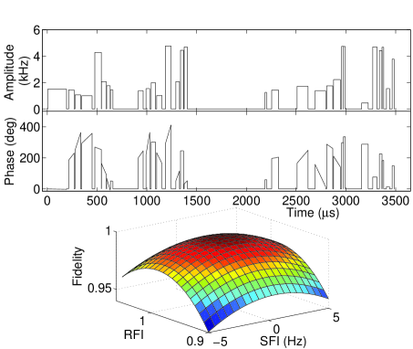
Figure 2: The SMP for QNGE: (top) amplitude vs time, (middle) phase vs time, and (bottom) fidelity vs RF inhomogeneity (RFI, 0.9 to 1.05 of the ideal field) and static field inhomogeneity (SFI, -5 Hz to 5 Hz). The 30-segment SMP has an average fidelity $F^{\prime}_{avg}=0.981.$

An SMP is a cascade of radio-frequency (RF) pulses numerically calculated based on the precise knowledge of the internal Hamiltonian of the qubit system and the target propagator fortunato ; navin . Given a target operator $U_{\mathrm{T}}$, Fortunato et al fortunato have described numerically searching an SMP propagator $U_{\mathrm{SMP}}$ based on four RF parameters for each segment $k$: duration ($\tau^{(k)}$), amplitude ($\omega_{A}^{(k)}$), phase ($\phi^{(k)}$) and frequency ($\omega_{F}^{(k)}$). We found that it is useful to add one more degree of freedom: after each pulse segment, we introduce a variable delay $\tau_{d}^{(k)}$. The delays are computationally inexpensive to optimize, easy and accurate to implement and make designing non-local gates easier. All the parameters are determined so as to maximize the fidelity

$$F=\mathrm{trace}\left[U_{\mathrm{T}}^{-1}\cdot U_{\mathrm{SMP}}\right]/M$$

where $U_{\mathrm{SMP}}$ is the propagator for the SMP, $M$ is the dimension of the operators and $s$ is the number of segments. A MATLAB package has been developed which uses the Nelder-Mead simplex algorithm as the maximization routine maheshsmp . The search constraints can be simplified if the input state is definitely known. The fidelity of an SMP specific to a known initial state $\rho_{\mathrm{in}}$ can be written as,

$$F^{\prime}=\frac{\mathrm{trace}\left[\rho_{T}\cdot\rho_{\mathrm{SMP}}\right]}{\sqrt{\mathrm{trace}\left[\rho_{T}^{2}\right]\cdot\mathrm{trace}\left[\rho_{\mathrm{SMP}}^{2}\right]}},$$ (4)

where $\rho_{T}=U_{\mathrm{T}}\cdot\rho_{\mathrm{in}}\cdot U_{\mathrm{T}}^{-1}$ and $\rho_{\mathrm{SMP}}=U_{\mathrm{SMP}}\cdot\rho_{\mathrm{in}}\cdot U_{\mathrm{SMP}}^{-1}$. The SMPs are made robust against the spatial inhomogeneous distributions of RF amplitudes and of static fields ($\Delta\omega_{i}$) by maximizing an average fidelity, $F^{\prime}_{avg}=\sum_{i}F^{\prime}(\omega_{iA},\Delta\omega_{i})$ nicrfi . Figure 2 shows a single SMP performing the full QNGE on the specific four-qubit system. Though it is possible to decompose the target propagator into several SMPs each corresponding to one or two-qubit gates, it is more efficient, at least for small spin systems, to design and execute a single robust SMP implementing the entire algorithm.

Figure 3: Molecular structure of 1-Chloro-2-iodobenzene (top-left), the elements of diagonalized Hamiltonian (top-right), and the energy level diagram with prominent transitions (bottom). The eigenstates are labeled as shown.

As the quantum register, we used the four ¹H spins of 1-Chloro-2-iodobenzene (CIB; Figure 3) (purchased from Sigma Aldrich^®) oriented in liquid crystal ZLI-1132 (purchased from Merck^®) forming a 10mM solution. All experiments were carried out on a 500 MHz Bruker Avance spectrometer at 300 K.

Figure 4 shows the ¹H NMR spectrum of the partially oriented CIB. The line widths of the various transitions range from 1.7 Hz to 4.0 Hz indicating coherence times ($T_{2}^{*}$ relaxation times) between 1.8 s and 0.7 s. The coherence times are sufficiently long to ignore relaxation effects in the design of the SMP.

The procedure for analyzing the NMR spectra of partially oriented systems has been well studied diehlvol6 ; emsleybook . We have developed a numerical procedure to iteratively determine the system Hamiltonian from its spectrum and a guess Hamiltonian maheshsamat . The 37 strongest transitions of the CIB spectrum were used and a unique fit was obtained. The mean frequency and intensity errors between the experimental and the calculated spectra are less than 0.1 Hz and 6% respectively. The elements of the diagonalized system Hamiltonian and the corresponding energy level diagram are shown in Figure 3.

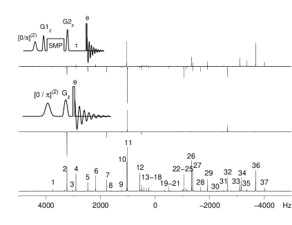
Figure 4: ¹H spectra of CIB obtained by applying a small angle pulse ($\theta=3^{\mathrm{o}}$) to the equilibrium state (bottom), $|0100\rangle\langle 0100|-|0000\rangle\langle 0000|$ POPS (middle), and QNGE (top). The transitions numbers correspond to those in Figure 3. The pulse sequences for POPS and QNGE are shown in insets. (by applying a transition-selective Gaussian $\pi$ pulse of 10 ms duration) Pulsed field gradients (G_z) are used to destroy coherence after POPS and after the SMP. In the QNGE experiment, the residual zero-quantum coherence are de-phased by a 32-step average over a random delay $\tau$ (between 0 and 10 ms).

In NMR-QIP, the initial states are not pure states but are pseudopure states that are isomorphic to pure states. The pseudopure states differ from the pure states by a uniform background population on all states. It is easier, however, to prepare a pair of pseudopure states (POPS) Fungpps . We prepared the pair $|0100\rangle\langle 0100|-|0000\rangle\langle 0000|$. The first term represents the desired initial state; the additional second part does not interfere with the QNGE experiment, because the operation IQFT, when acted on $|00\rangle$, creates a uniform superposition of the ancilla qubits. Such a state is invariant under the $f(x)\oplus_{N_{0}}$ operation and therefore the output state corresponding to $|0000\rangle\langle 0000|$ is independent of the oracle $U_{f}$. The inset at the center of Figure 4 shows the pulse sequence for preparing POPS and the corresponding spectrum. The POPS spectrum is obtained by linear detection pulse after inverting transition 2 and subtracting from the resulting spectrum the linearly detected spectrum of the equilibrium state.

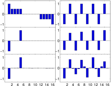
Figure 5: Bar-plots showing the diagonal elements of the density matrix in the eigenbasis: equilibrium (top left), simulated POPS (middle left), experimental POPS (bottom left), theoretical output of QNGE (top right), simulated output (with the SMP shown in Figure 2; middle right), and experimental output of the quantum algorithm (bottom right).

Since we use eigenbasis as the computational basis, the projective measurement on to the computational basis is equivalent to measurement of populations after destroying the coherence. First we dephase the coherence by using a pulsed field gradient (PFG). A PFG does not efficiently dephase homonuclear zero-quantum coherence. Therefore we use a random delay (in between 0 and 10 ms) after the PFG and average over several (32) transients. The populations are then measured using a linear detection (small flip-angle) pulse ernstbook . Using the normalization condition, there are 15 unknowns for the 16 eigenstates. The results of the diagonal-tomography obtained by the mean of three sets each of 15 linearly independent transitions are shown in Figure 5.

After the projective measurement in the eigenbasis at the end of the quantum algorithm, the input qubits are in the state $|10\rangle$ encoding the gradient $\nabla f=2$, while the ancilla qubits have equal probability in all possible states. Therefore, the theoretical output diagonal state of the combined system is $I_{an}\otimes(|10\rangle\langle 10|-|00\rangle\langle 00|$), where $I_{an}$ is the identity operator for the ancilla qubits and the two parts in the parenthesis correspond to the two parts of the POPS.

The diagonal correlation $C$ between the theoretical density matrix ($\rho_{\mathrm{T}}$) and the experimental density matrix ($\rho_{\mathrm{E}}$), is defined as

$$C=\frac{\mathrm{trace}[|\rho_{\mathrm{T}}|\cdot|\rho_{\mathrm{E}}|]}{\sqrt{\mathrm{trace}[|\rho_{\mathrm{T}}|^{2}]\cdot\mathrm{trace}[|\rho_{\mathrm{E}}|^{2}]}},$$ (5)

where $||$ denotes extraction of the diagonal part. The average diagonal correlations were 0.999 and 0.979 for the POPS and the result of the QNGE, respectively. The lower value of the latter may be attributed to decoherence and spectrometer nonlinearities.

In conclusion, we have demonstrated quantum computation on the eigenbasis of system Hamiltonian using coherent control techniques. As an example, we described the first implementation of Jordan’s algorithm for numerical gradient estimation. Compared to the usual approach using weakly coupled systems, the present method using strongly dipolar coupled systems yields significantly faster execution times and is therefore less susceptible to decoherence effects. From molecular and spectroscopic considerations a combination of homo and heteronuclear spins in either liquid crystalline or molecular single crystalline environments is a natural way to build larger qubit-systems (with $>10$ qubits). The coherent control of strongly dipolar coupled systems then becomes important and the present work is the first step in this direction. We believe that the coherent control techniques demonstrated here for dipolar coupled nuclear spins will turn out to be essential also for other solid-state implementations of quantum information processing.

- (1) D. P. DiVincenzo, Fortschr. Phys. 48, 771 (2000).
- (2) C. Ramanathan, N. Boulant, Z. Chen, D. G. Cory, I. L. Chuang, M. Steffen Quantum Information Processing, 3, 15 (2004).
- (3) J. Baugh, O. Moussa, C. A. Ryan, R. Laflamme, C. Ramanathan, T. F. Havel, and D. G. Cory Phys. Rev. A 73, 022305 (2006).
- (4) R. R. Ernst, G. Bodenhausen, and A. Wokaun, Principles of Nuclear Magnetic Resonance in One and Two Dimensions, Oxford Science Publications, (1987).
- (5) M. H. Levitt, Spin Dynamics, J. Wiley and Sons Ltd., 2002.
- (6) T. S. Mahesh, N. Sinha, A. Ghosh, R. Das, N. Suryaprakash, M. H. Levitt, K. V. Ramanathan, and A. Kumar, Curr. Sci. 85, 932 (2003); Also available at LANL ArXiv quant-ph:0212123.
- (7) NMR-Basic Principles and Progress, P. Diehl, H. Kellerhals, and E. Lustig, Eds. P. Diehl, E. Fluck and R. Kosfeld, Springer-Verlog, New York, Vol. 6, 1972
- (8) NMR spectroscopy using liquid crystal solvents, J. W. Emsley and J. C. Lindon, Pergamon Press, 1975.
- (9) S. P. Jordan, Phys. Rev. Lett. 95, 050501 (2005).
- (10) M. A. Nielsen and I. L. Chuang, Quantum Computation and Quantum Information, Cambridge University Press, 2002.
- (11) E. M. Fortunato, M. A. Pravia, N. Boulant, G. Teklemariam, T. F. Havel and D. G. Cory, J. Chem. Phys. 116, 7599 (2002).
- (12) N. Khaneja, T. Reiss, C. Kehlet, T. S. Herbrüggen, and S. J. Glasser, J. Magn. Reson. 172, 296 (2005).
- (13) T. S. Mahesh and D. Suter, to be published elsewhere.
- (14) N. Boulant, J. Emerson, T. F. Havel, S. Furuta and D. G. Cory, J. Chem. Phys. 121, 2955 (2004).
- (15) T. S. Mahesh and D. Suter, to be published elsewhere.
- (16) B. M. Fung, Phys. Rev. A. 63, 022304 (2001).