Loschmidt Echo and Berry phase of the quantum system coupled to the $XY$ spin chain: Proximity to quantum phase transition

Abstract

We study the Loschmidt echo (LE) of a coupled system consisting of a central spin and its surrounding environment described by a general XY spin-chain model. The quantum dynamics of the LE is shown to be remarkably influenced by the quantum criticality of the spin chain. In particular, the decaying behavior of the LE is found to be controlled by the anisotropy parameter of the spin chain. Furthermore, we show that due to the coupling to the spin chain, the ground-state Berry phase for the central spin becomes nonanalytical and its derivative with respect to the magnetic parameter $\lambda$ in spin chain diverges along the critical line $\lambda=1$, which suggests an alternative measurement of the quantum criticality of the spin chain.

Quantum phase transition (QPT), which is closely associated with the occurrence of nonanalyticity of the ground-state energy as a function of the coupling parameters in the system’s HamiltonianSach , are of extensive current interest, mainly in condensed matter physics because they are not only at the origin of unusual finite temperature properties but also promote the formation of new states of matter like unconventional superconductivity in heavy-fermion systemMathur . In the parameter space, the points of nonanalyticity of the ground-state energy density are referred to as critical points and define QPT. At these points one typically witnesses the divergence of the length associated with the two-point correlation function of some relevant quantum field. In experiments QPT has been extensively studied in the heavy-fermion compoundsLace ; Gege . Recently, QPT has drawn a considerable interest in other fields of physics. More specifically QPT has been studied by analyzing scaling, asymptotical behavior and extremal points of various entanglement measuresOst ; Vidal ; Chen ; Gu ; Wu . The connection between geometric Berry phase (BP) and QPT for the case of spin-XY model has also been studiedCar ; Zhu ; Ham , through which a remarkable relation between the BP and criticality of spin chains is established. In addition, a characterization of QPT in terms of the overlap between two ground states obtained for two different values of external parameters has been presentedZarnidi .

Another way to study quantum criticality is to investigate quantum dynamics of the many-body systems. Recently, Sengupta et al.Seng have studied time evolution of the Ising order correlations under a time-dependent transverse field and shown that the order parameter is best enhanced in the vicinity of the quantum critical point. Quan et al.Quan have studied transition dynamics of a quantum two-level system from a pure state to a mixed one induced by the quantum criticality of the surrounding many-body system. They have shown that the decaying behavior of the LE is best enhanced by the QPT of the surrounding system. Yi et al.Yi have reported the relation between the Hahn spin echo of a spin-1/2 particle and QPT in a spin chain which is coupled to the particle. It is expected that further work associated with the dynamical measurement of QPT via a coupling to the central probe system will be reported afterwards. From this aspect a thorough theoretical investigation of the quantum dynamics in QPT regime, including the various kinds of spin-chain models, is necessary and will be helpful for future experimental references.

In this paper, we present a theoretical study of the behavior of the Loschmidt echo (LE) of a coupled spin system which consists of two quantum subsystems. One subsystem is characterized by a spin-1/2 Hamiltonian, which denotes the general two-level particles. We call this subsystem the central spin, in the sense that this spin plays the role of measuring apparatus. Whereas the other subsystem plays the role of surrounding many-body environment and is modeled by a general $XY$ spin chain in a transverse magnetic field. The present study is directly motivated by the recent theoretical reportQuan that the quantum critical behavior of environmental system strongly affects its capability of enhancing the decay of LE. Here we extend the Ising model used in Ref.[15] for simulating the environmental subsystem to the more general XY model. Compared to the Ising model, the XY model is parametrized by $\gamma$ and $\lambda$ [see Eq. 1(b) below]. Two distinct critical regions appear in parameter space: the segment $(\gamma,\lambda)=(0,(0,1))$ for the $XX$ spin chain and the critical line $\lambda_{c}=1$ for the whole family of the $XY$ modelSach . The behavior of decaying enhancement of the LE calculated in Ref.[15] can be used as a measure of the presence of the quantum criticality of the Ising spin chain. It remains yet to be exploited whether this decaying enhacement sustains in the whole critical regions for the $XY$ model.

The other interest in this paper is to study the BP properties of the coupled system. Instead of investigating the BP of the environmental $XY$ spin chain which has been previously studiedCar ; Zhu ; Ham , we focus our attention to the ground-state BP of the central quantum subsystem. Due to the coupling, it is expected that the quantum criticality of the surrounding $XY$ spin chain will influence the BP of the central spin, which is found in this paper to be close proximity to the nonanalytical and divergent behavior of QPT of the environmental spin chain in the critical region.

We consider a two-level quantum system (central spin) transversely coupled to a environmental spin chain which is described by the one-dimensional $XY$ model. The corresponding Hamitonian is given by $H=H_{C}+H_{E}+H_{I}$, where (we take $\hbar=1$)

$$H_{C}=\mu\sigma^{z}/2+\nu\sigma^{x}/2,$$ (1a)

$$H_{E}=-\sum_{l}^{N}\left(\frac{1+\gamma}{2}\sigma_{l}^{x}\sigma_{l+1}^{x}+\frac{1-\gamma}{2}\sigma_{l}^{y}\sigma_{l+1}^{y}+\lambda\sigma_{l}^{z}\right),$$ (1b)

$$H_{I}=\frac{g}{N}\overset{N}{\underset{l=1}{\sum}}\sigma^{z}\sigma_{l}^{z}.$$ (1c)

Here the Pauli matrices $\sigma^{\alpha}$ ($\alpha=x,y,z$) and $\sigma_{l}^{\alpha}$ are used to describe the central spin and the environmental spin-chain subsystems, respectively. The parameter $\lambda$ in $H_{E}$ is the intensity of the magnetic filed applied along $z$-axis, and $\gamma$ measures the anisotropy in the in-plane interaction. It is well known that the $XY$ model in Eq. (1b) encompasses two other well-known spin models: it turns into transverse Ising chain for $\gamma=1$ and the $XX$ chain for $\gamma=0$. $H_{I}$ gives the coupling between the central spin and the surrounding spin chain. The above employed model is similar to the Hepp-Coleman modelHepp ; Bell or its generalizationNaka ; Cini ; Sun .

As for quantum criticality in the $XY$ model, there are two universality classes depending on the anisotropy $\gamma$. The critical features are characterized in terms of a critical exponent $\nu$ defined by $\xi\sim|\lambda-\lambda_{c}|^{-\nu}$ with $\xi$ representing the correlation length. For any value of $\gamma$, quantum criticality occurs at a critical magnetic field $\lambda_{c}=1$. For the interval $0<\gamma\leq 1$ the model belongs to the Ising universality class characterized by the critical exponent $\nu=1$, while for $\gamma=0$ the model belongs to the $XX$ universality class with $\nu=1/2$Sach .

Following Ref.[15], we assume that the central spin is initially in a superposition state $|\phi_{S}(0)\rangle=c_{g}|g\rangle+c_{e}|e\rangle$, where $|g\rangle=\left(\sin\frac{\theta}{2},-\cos\frac{\theta}{2}\right)^{\text{T}}$ and $|e\rangle=\left(\cos\frac{\theta}{2},\sin\frac{\theta}{2}\right)^{\text{T}}$ with $\theta=\tan^{-1}(\nu/\mu)$ are ground and excited states of $H_{C}$, respectively. The coefficients $c_{g}$ and $c_{e}$ satisfy the normalization condition, $|c_{g}|^{2}+|c_{e}|^{2}=1$. Then the evolution of the $XY$ spin chain initially prepared in $|\varphi(0)\rangle$, will split into two branches $|\varphi_{\alpha}(t)\rangle=\exp(-iH_{\alpha}t)|\varphi(0)\rangle$ ($\alpha=g,e$), and the total wave function is obtained as $|\psi(t)\rangle=c_{g}|g\rangle\otimes|\varphi_{g}(t)\rangle+c_{e}|e\rangle\otimes|\varphi_{e}(t)\rangle$. Here, the evolutions of the two branch wave functions $|\varphi_{\alpha}(t)\rangle$ are driven, respectively, by the two effective Hamiltonians

$$H_{g}=\langle g|H|g\rangle=H_{E}-\delta\underset{l=1}{\overset{N}{{\displaystyle\sum}}}\sigma_{l}^{z}-\Delta,$$ (2a)

$$H_{e}=\langle e|H|e\rangle=H_{E}+\delta\underset{l=1}{\overset{N}{{\displaystyle\sum}}}\sigma_{l}^{z}+\Delta,$$ (2b)

where $\Delta=\sqrt{\mu^{2}+\nu^{2}}/2$ and $\delta=g\cos\theta/N$. Obviously, both $H_{g}$ and $H_{e}$ describe the $XY$ model in a transverse field, but with a tiny difference in the field strength. The central spin in two different states $|g\rangle$ and $|e\rangle$ will exert slightly different backactions on the surrounding spin chain, which manifests as two effective potentials $V_{g}=-\delta\underset{l=1}{\overset{N}{{\displaystyle\sum}}}\sigma_{l}^{z}$ and $V_{e}=\delta\underset{l=1}{\overset{N}{{\displaystyle\sum}}}\sigma_{l}^{z}$. This difference results in the decay of the LEKark defined asQuan

$$L(t)=|\langle\varphi_{g}(t)|\varphi_{e}(t)\rangle|^{2}$$ (3)

The LE has been proved to be conveniently related to depicting quantum decoherence of the central systemQuan : consider the purity definedKark by $P=$Tr${}_{C}(\rho_{C}^{2})=$Tr${}_{C}\{[$Tr${}_{E}\rho(t)]^{2}\}$. Here $\rho(t)=|\psi(t)\rangle\langle\psi(t)|$, and Tr_C(E) means tracing over the degrees of freedom for the central spin (environmental spin chain). A straightforward calculation reveals the relationship between the LE and the purity as $P=1-2|c_{g}c_{e}|^{2}\left[1-L(t)\right]$Quan . This equation indicates that the purity depends on the initial state of the central spin and the surrounding spin chain. For simplicity, we assume that the spin chain subsystem begins with its ground state. In the following discussion, we will focus on the quantum dynamics of the LE in the different parameter regions. In particular, the decay problem of LE induced by the coupling of the central spin and its surrounding spin chain, as has been discussed in Ref.[15] for the special case of Ising model, will be fully studied in the ($\gamma,\lambda$)-space.

To diagonalize the effective Hamiltonians $H_{i}$ ($i=g,e$), we follow the standard procedureSach by defining the conventional Jordan-Wigner (JW) transformation

$$\sigma_{l}^{x}=\underset{m<l}{\prod}(1-2a_{m}^{+}a_{m})\left(a_{l}+a_{l}^{+}\right),$$ (4a)

$$\sigma_{l}^{y}=-i\underset{m<l}{\prod}(1-2a_{m}^{+}a_{m})\left(a_{l}-a_{l}^{+}\right),$$ (4b)

$$\sigma_{l}^{z}=1-2a_{l}^{+}a_{l}.$$ (4c)

which maps spins to one-dimensional spinless fermions with creation (annihilation) operators $a_{l}^{+}$ ($a_{l}$). After a straightforward derivation, the effective Hamiltonians read

$$H_{i} =-\overset{N}{\underset{l=1}{\sum}}[(a_{l+1}^{+}a_{l}+a_{l}^{+}a_{l+1})+\gamma(a_{l+1}a_{l}+a_{l}^{+}a_{l+1}^{+})$$ (5)

$$+\left(\lambda+\kappa_{i}\delta\right)(1-2a_{l}^{+}a_{l})]-\kappa_{i}\Delta,$$

where $\kappa_{g}=-\kappa_{e}=1$. Next we introduce Fourier transforms of the fermionic operators described by $d_{k}=\frac{1}{\sqrt{N}}\sum_{l}a_{l}e^{-i2\pi lk/N}$ with $k=-M,..,M$, $M=N/2$. The Hamitionians (4) can be diagonalized by transforming the fermion operators in momentum space and then using the Bogoliubov transformation. The results are

$$H_{i}=\sum_{k}2\Lambda_{k,i}(b_{k,i}^{+}b_{k,i}-1/2)-\kappa_{i}\Delta,$$ (6)

where the energy spectrums $\Lambda_{k,i}$ ($i=g,e$) are given by

$$\Lambda_{k,i}=\sqrt{\epsilon_{k,i}^{2}+\gamma^{2}\sin^{2}\frac{2\pi k}{N}}\text{ with }\epsilon_{k,i}=\lambda-\cos\frac{2\pi k}{N}+\kappa_{i}\delta,$$ (7)

and the corresponding Bogoliubov-transformed fermion operators are defined by

$$b_{k,i}=\cos\frac{\theta_{k}^{(i)}}{2}d_{k}-i\sin\frac{\theta_{k}^{(i)}}{2}d_{-k}^{+}$$ (8)

with angles $\theta_{k}^{(i)}$ satisfying $\cos\theta_{k}^{(i)}=\epsilon_{k,i}/\Lambda_{k,i}$. It is straightforward to see that the two sets of normal modes are related by the equation $b_{k,e}=(\cos\alpha_{k})b_{k,g}-i(\sin\alpha_{k})b_{-k,g}^{+}$ where $\alpha_{k}=(\theta_{k}^{(e)}-\theta_{k}^{(g)})/2$.

The ground state $|G\rangle$ of $H_{i}$ is the vacuum of the fermionic modes described by $b_{k,i}|G\rangle_{i}=0$, and can be written as $|G\rangle_{i}={\textstyle\prod\nolimits_{k=1}^{M}}\left(\cos\frac{\theta_{k}^{(i)}}{2}|0\rangle_{k}|0\rangle_{-k}+i\sin\frac{\theta_{k}^{(i)}}{2}|1\rangle_{k}|1\rangle_{-k}\right)$, where $|0\rangle_{k}$ and $|1\rangle_{k}$ denote the vacuum and single excitation of the $k$th mode, $d_{k}$, respectively. Note that the ground state is a tensor product of states, each lying in the two-dimensional Hilbert space spanned by $|0\rangle_{k}|0\rangle_{-k}$ and $|1\rangle_{k}|1\rangle_{-k}$. From the relationship between the two Bogoliubov modes $b_{k,e}$ and $b_{k,g}$, one can see that the ground state $|G\rangle_{g}$ of the effective Hamiltonian $H_{g}$ can be obtained from the ground state $|G\rangle_{e}$ of $H_{e}$ by the transformation $|G\rangle_{g}={\textstyle\prod\nolimits_{k=1}^{M}}(\cos\alpha_{k}+i\sin\alpha_{k}b_{k,e}^{+}b_{-k,e}^{+})|G\rangle_{e}$.

Now we suppose that the $XY$ spin chain is initially in the ground state of $H_{g}$, i.e., $|\varphi(0)\rangle=|G\rangle_{g}$. Then our present task is to derive the explicit expression for LE. First one notices that the LE in Eq. (3) can be rewritten as

$$L(t) =|\langle\varphi_{g}(t)|\varphi_{e}(t)\rangle|^{2}=|_{g}\langle G|e^{-iH_{e}t}|G\rangle_{g}|^{2}$$ (9)

$$=|_{e}\langle G|{\textstyle\prod\nolimits_{k}}(\cos\alpha_{k}-i\sin\alpha_{k}b_{-k,e}b_{k,e})e^{-iH_{e}t}{\textstyle\prod\nolimits_{k}}(\cos\alpha_{k}+i\sin\alpha_{k}b_{k,e}^{+}b_{-k,e}^{+})|G\rangle_{e}|^{2},$$

where the dynamical phase in $|\varphi_{g}(t)\rangle$ contributed by the time evolution operator $e^{-iH_{g}t}$ has been eliminated by the arithmetic module operation in $L(t)$. By using the identity $e^{-iH_{e}t}b_{k,e}^{+}e^{iH_{e}t}=b_{k,e}^{+}e^{-i2\Lambda_{k,e}t}$ and after a straightforward derivation, one obtains the expression for $L(t)$ as follows

$$L(t) =|_{e}\langle G|{\textstyle\prod\nolimits_{k}}(\cos\alpha_{k}-i\sin\alpha_{k}b_{-k,e}b_{k,e})(\cos\alpha_{k}+ie^{-i4\Lambda_{k,e}t}\sin\alpha_{k}b_{k,e}^{+}b_{-k,e}^{+})|G\rangle_{e}|^{2}$$ (10)

$$=|{\textstyle\prod\nolimits_{k}}(\cos^{2}\alpha_{k}+\sin^{2}\alpha_{k}e^{-i4\Lambda_{k,e}t})|^{2}$$

$$={\textstyle\prod\nolimits_{k=1}^{M}}\left[1-\sin^{2}\left(2\alpha_{k}\right)\sin^{2}\left(2\Lambda_{k,e}t\right)\right].$$

Remarkably, the expression for $L(t)$ based on $XY$ spin chain is formally same as that based on Ising model which has been previously reportedQuan . The difference comes from the time-dependent phase factor, which in the present case is the energy spectrum $2\Lambda_{k,e}$ of $XY$ spin-chain characterized by the effective Hamiltonian $H_{e}$, instead of Ising model given in Ref.Quan . Due to the obvious difference in the energy spectrum between $XY$ model and Ising model, one may expect that the behavior of the LE in the present case will include new features characteristic of the $XY$ model.

Since each factor $F_{k}$ in Eq. (10) has a norm less than unity, we may expect $L(t)$ to decrease to zero in the large $N$ limit under some reasonable conditions. This kind of factorized structure was first discovered and systematically studiedSun in developing the quantum measurement theory in classical or macroscopic limit and has been applied to analyze the universality of decoherence influence from environment on quantum computingSun2 . Now we study in detail the critical behavior of of LE near the critical point $\lambda_{c}=1$ for finite lattice size $N$ of spin chain. Following Ref.Quan , let us first make a heuristic analysis of the features of the LE. For a cutoff frequency $K_{c}$ we define the partial product for the LE

$$L_{c}(t)={\textstyle\prod\nolimits_{k=1}^{K_{c}}}F_{k}\geq L_{c}(t),$$ (11)

and the corresponding partial sum $S(t)=\ln L_{c}\equiv-{\textstyle\sum\nolimits_{k=1}^{K_{c}}}|\ln F_{k}|$. For small $k$ one has

$$\Lambda_{k,e}\approx|\lambda-1-\delta|+O(k^{2}),$$ (12)

and

$$\sin^{2}\left(2\alpha_{k}\right)\approx\frac{4\pi^{2}4\gamma^{2}\delta^{2}k^{2}}{N^{2}(\lambda-\delta-1)^{2}(\lambda+\delta-1)^{2}}.$$ (13)

As a result, if $K_{c}$ is small enough one has

$$S(t)=-\frac{4E(N_{c})\gamma^{2}\delta^{2}\sin^{2}\left(2t|\lambda-\delta-1|\right)}{(\lambda-\delta-1)^{2}(\lambda+\delta-1)^{2}},$$ (14)

where $E(N_{c})=4\pi^{2}N_{c}(N_{c}+1)(2N_{c}+1)/(6N^{2})$. In this case, it then follows that for a fixed $t$,

$$L_{c}(t)\approx\exp(-\tau t^{2})$$ (15)

when $\lambda\rightarrow\lambda_{c}=1$, where $\tau=16E(N_{c})\gamma^{2}\delta^{2}/(\lambda+\delta-1)^{2}$.

From Eq. (15) it may be expected that when $N$ is large enough and $\lambda$ is adjusted to the vicinity of the critical point $\lambda_{c}=1$, the LE will exceptionally vanish with time. In the thermodynamic limit, i.e., the number $N$ of sites approaching infinite while the length of spin chain keeping a constant, $\tau$ seems to tend to zero and thus the approximate expression $L_{c}(t)$ remains unity without any decay. This implies that our heuristic analysis cannot apply to the case of thermodynamic limit, in which case the small-$k$ approximation becomes invalid. Thus to reveal the close relationship between the decaying behavior of LE and QPT which occur only in the thermodynamic limit, all $k$-components of $F_{k}$ in Eq. (11) should be included. On the other side, for a practical system used to demonstrate the QPT-induced decay of the LE, the particle number $N$ is large, but finite, and then the practical $\tau$ in Eq. (15) does not vanish.

Figure 1: (color online). (a) The LE as a function of magnetic intensity $\lambda$ and time $t$ for Ising ($\gamma=1.0$) spin-chain size $N=100$; (b) The LE as a function of time for different values of N for Ising spin chain.

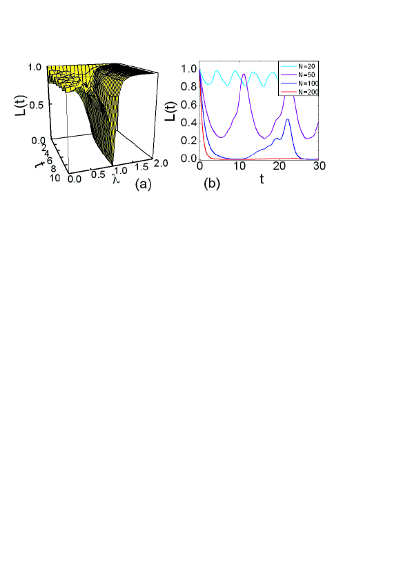
Figure 1(a) shows the numerical result of the LE in Eq. (10) as a function of magnetic intensity $\lambda$ and time $t$ for $N=100$, $\delta=0.05$, and $\gamma=1.0$ (i.e., the case of Ising model). One can see that when the value of $\lambda$ is larger or smaller than that of $\lambda_{c}$, the LE in time domain is characterized by an oscillatory localization behavior. When the amplitude of $\lambda$ approaches to $\lambda_{c}$, then the degree of localization of $L(t)$ is decreased to zero. The fundamental change occurs at critical point of QPT, i.e., $\lambda=\lambda_{c}=1$. At this point, as revealed in Fig. 1(a), the LE evolves from unity to zero in a very short time. Figure 1(b) shows the time evolution of LE for different values of lattice size at critical point $\lambda=1$ of Ising model. One can see that the LE decays more rapidly by increasing the size $N$ of spin chain. Also the decaying amplitude is increased with increasing $N$.

Figure 2: The LE as a function of time for $\lambda=1.0$ and different values of anisotropy $\gamma$. The other parameters are chosen to be $N=100$, $\delta=0.05$.

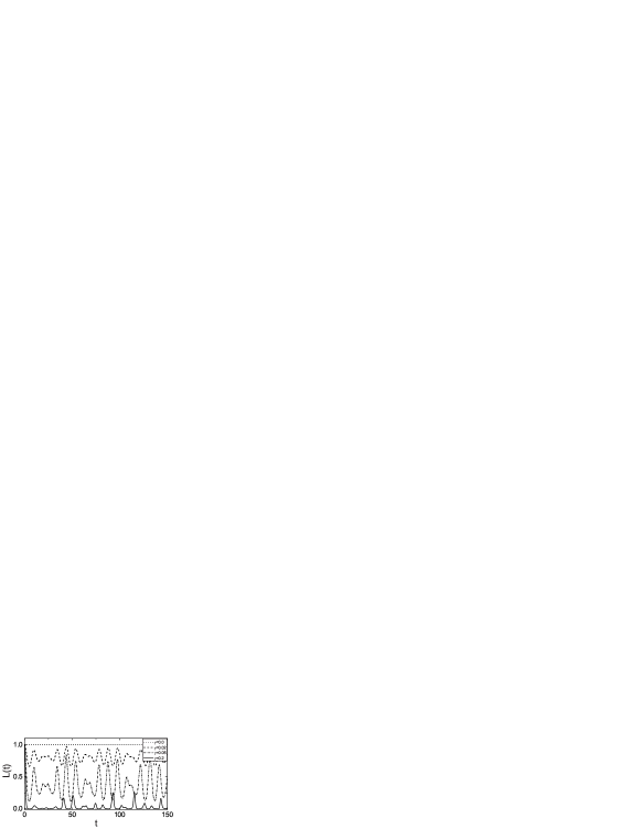
Figure 2 shows the LE as a function of time for different values of anisotropy parameter $\gamma$ in the quantum critical region ($\lambda=\lambda_{c}$). In the extreme anisotropy limit, i.e., for the $XX$ spin model ($\gamma=0$), one can see from Fig. 2 that the LE completely remains to be unity during time evolution. This full localization behavior can also be seen from the analytic expression Eq.(14), in which $\tau=0$ for $\gamma=0$, indicating no decay in the LE, regardless of the variation of $\lambda$ and the size of spin chain. As a consequence, the purity $P$ of the central spin remains unity; the coupling induced decoherence disappears for the $XX$ spin chain. In this case, the quantum criticality behavior of the surrounding spin chain dose not affect the localization behavior of the LE for the central spin. By smoothly tuning the value of $\gamma$ little out of $XX$ model, as shown in Fig. 2, the behavior of the LE begins to be characterized by an interplay of the decay in a short time and the oscillations in the subsequent evolution. The oscillations are featured by a superposition of the collapses and the revivals. The amplitude of the oscillations is decreased with increasing the value of $\gamma$. Further increasing the value of $\gamma$ will, as one can see from Fig. 2, lead to the complete decay of the LE without prominent revivals during the whole time evolution. Therefore, the decay of the LE and its proximity to the quantum criticality can be tuned by the anisotropy parameter $\gamma$.

Now we turn to study the behavior of the ground-state BP for the central spin. Due to the coupling, it is expected that the BP for the central spin will be profoundly influenced by the occurrence of QPT in spin-chain environment.

Similar to the above discussions, it is supposed that the $XY$ spin chain is adiabatically in the ground state $|G(\{\theta_{k}\})\rangle_{g}$ of $H_{g}$, which is parameterized by the series $\{\theta_{k}\}$ in the ground state. Thus the effective mean-field Hamiltonian for the central spin is given by

$$H_{eff} =H_{S}+_{g}\langle G|H_{I}|G\rangle_{g}$$ (16)

$$=\left(\frac{\mu}{2}+\frac{2g}{N}\sum_{k=1}^{M}\cos\theta_{k}^{(g)}\right)\sigma^{z}+\frac{\nu}{2}\sigma^{x}.$$

In order to generate a BP for the central spin, we change the Hamiltonian by means of a unitary transformation:

$$U(\phi)=\exp\left(-i\frac{\phi}{2}\sigma_{z}\right),$$ (17)

where $\phi$ is a slowly varying parameter, changing from $0$ to $2\pi$. The transformed Hamiltonian can be written as

$$H_{eff}(\phi) =U^{+}(\phi)H_{eff}U(\phi)$$ (18)

$$=\left(\frac{\mu}{2}+\frac{2g}{N}\sum_{k=1}^{M}\cos\theta_{k}^{(g)}\right)\sigma^{z}+\frac{\nu}{2}(\sigma^{x}\cos\phi-\sigma^{y}\sin\phi).$$

The eigen-energies of the effective Hamiltonian for the central spin are given by

$$E_{e,g}=\pm\sqrt{\left(\frac{\mu}{2}+\frac{2g}{N}\sum_{k=1}^{M}\cos\theta_{k}^{(g)}\right)^{2}+\frac{\nu^{2}}{4}}.$$ (19)

The corresponding eigenstates are

$$|g\rangle=\binom{\sin\frac{\theta}{2}}{-\cos\frac{\theta}{2}e^{-i\phi}},|e\rangle=\binom{\cos\frac{\theta}{2}}{\sin\frac{\theta}{2}e^{-i\phi}},$$ (20)

where $\sin\theta=\nu/2E_{e}$.

The acquired ground-state BP for the central spin by varying $\phi$ from zero to $2\pi$ is given by

$$\beta_{g} =i\int_{0}^{2\pi}\langle g|\frac{\partial}{\partial\phi}|g\rangle=\pi(1+\cos\theta)$$ (21)

$$=\pi\left(1+\frac{\mu+4gf(\lambda,\gamma,N)}{\sqrt{[\mu+4gf(\lambda,N)]^{2}+\nu^{2}}}\right),$$

where we have defined $f(\lambda,\gamma,N)=\frac{1}{N}\sum_{k=1}^{M}\cos\theta_{k}^{(g)}$. In the thermodynamic limit, $N\rightarrow\infty$, the summation in $f(\lambda,\gamma,N)$ can be replaced by the integral as follows:

$$f(\lambda,\gamma,N)|_{N\rightarrow\infty}=\frac{1}{2\pi}\int_{0}^{\pi}\frac{\lambda-\cos\varphi}{\sqrt{(\lambda-\cos\varphi)^{2}+\gamma^{2}\sin^{2}\varphi}}d\varphi.$$ (22)

The BP $\beta_{g}$ for the central spin is closely related with QPT of its coupled spin-chain subsystem. To manifest this, we plot in Fig. 3 the BP $\beta_{g}$ and its derivative $d\beta_{g}/d\lambda$ with respect to the field strength $\lambda$ as a function of spin-chain parameters $\lambda$ and $\gamma$.

Figure 3: (color online). (a) Ground-state BP of the central spin and (b) its $\lambda$-derivative as a function of spin-chain parameters $\lambda$ and $\gamma$ in the thermodynamic limit. The other parameters are chosen to be $\mu=0.1$, $\nu=2.0$, and $g=0.5$.

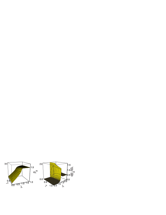
One can see that given the value of $\gamma$, the BP of the central spin increases with increasing the field strength $\lambda$. After passing through the critical line $\lambda_{c}=1$, the BP $\beta_{g}$ arrives at a stable value which turns out to be determined by the specific values of central-spin parameters $\mu$ and $\nu$. The nonanalytic property of BP and its $\lambda$-derivative along the whole critical line can be clearly seen from Fig. 3. Thus a nonanalytic ground-state GP $\beta_{g}$ and the corresponding anomaly in its derivative $d\beta_{g}/d\lambda$ for the central spin also witness QPT of the coupling spin-chain subsystem.

To help further illustration, let us consider the most discontinuous case of $XX$ spin model ($\gamma=0$). In the thermodynamic limit, the function $f$ [Eq. (22)] occurred in the expression of $\beta_{g}$ can be obtained explicitly for $\gamma=0$ as $f=1/2-\arccos(\lambda)/\pi$ when $\lambda\leq 1$ and $f=1/2$ when $\lambda>1$. Thus the BP of the central spin is given by

$$\beta_{g}\bigr{|}_{N\rightarrow\infty}=\left\{\begin{array}[c]{l}\pi\left(1+\frac{\mu+2g[1-2\arccos(\lambda)/\pi]}{\sqrt{\left(\mu+2g[1-2\arccos(\lambda)/\pi]\right)^{2}+\nu^{2}}}\right)\text{ \ \ (}\lambda\leq 1\text{)}\\ \pi\left(1+\frac{\mu+2g}{\sqrt{\left(\mu+2g\right)^{2}+\nu^{2}}}\right)\text{ \ \ \ \ \ \ \ \ \ \ \ \ \ \ \ \ \ \ \ (}\lambda>1\text{)}\end{array}\right.,$$ (23)

which clearly shows a discontinuity at $\lambda=\lambda_{c}=1$. On the other side, one can see that the value of function $f(\lambda,\gamma,N)$ in $\beta_{g}$ is always trivial for $\gamma=0$ and every finite lattice size $N$, since $\theta_{k}^{(g)}=0$ or $\pi$ for every $k$. The difference between the finite and infinite lattice size can be understood, as has been first demonstrated in Ref.Zhu , from the two limits $N\rightarrow\infty$ and $\gamma\rightarrow 0$.

Figure 4: (color online). $\lambda$-dependence of ground-state BP of the central spin coupled to a $XX$ spin chain ($\gamma=0$) with different chain sizes $N$. The other parameters are the same as used in Fig. 3.

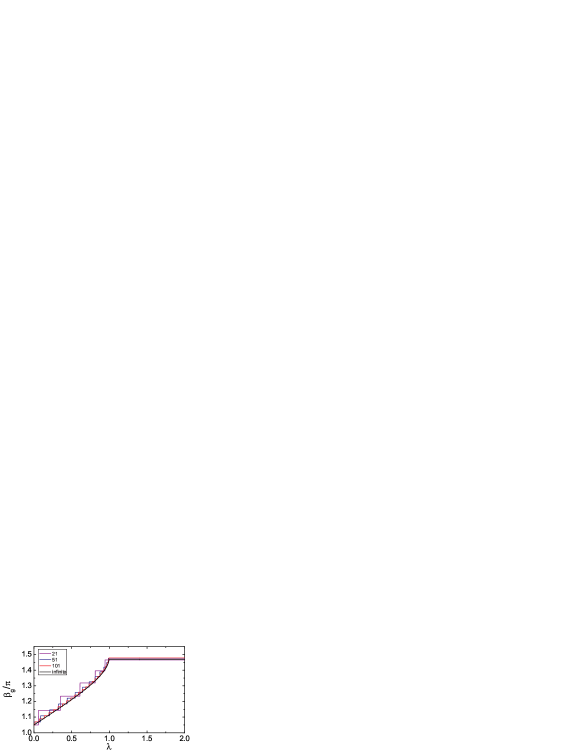
We plot in Fig. 4 the numerical results of the BP $\beta_{g}$ for different values of spin-chain size $N$, in comparison with the result for the thermodynamic limit. One can see that the BP of the central spin displays a multi-step like behavior for the small values of spin chain size $N$. By increasing $N$, the BP approaches towards the case of thermodynamic limit with nonanalyticity only at $\lambda_{c}$. We notice that the multi-step behavior of $\beta_{g}$ for finite lattice size is a unique feature of the $XX$ model ($\gamma=0$), and will be completely washed out by deviation of $\gamma$ from zero.

Figure 5: (color online). $\lambda$-dependence of $d\beta_{g}/d\lambda$ for the central spin which is coupled to the Ising spin chain ($\gamma=1$) with different chain sizes $N=15,51,251,501,\infty$. The behavior of $d\beta_{g}/d\lambda$ for the central spin reflects QPT of spin chain. With increasing the chain sizes, the peak becomes more pronounced. The inset shows the size scaling of the position of the peak occurred in $d\beta_{g}/d\lambda$ (circles) and in function $f(\lambda,\gamma,N)$ (squares).

To further understand the relationship between BP of the central spin and quantum criticality of the coupled spin chain, we calculate the derivative $d\beta_{g}/d\lambda$ as a function of $\lambda$ for $\gamma=1$ (Ising model) and different lattice sizes. The results are plotted in Fig. 5. Two prominent features can be seen: (i) The derivative $d\beta_{g}/d\lambda$ of GP is peaked around $\lambda=1$, as in the thermodynamic limit shown in Fig. 3(b). The amplitude of the peak is prominently enhanced by increasing the lattice size of spin chain; (ii) The accurate position $\lambda_{m}$ of the peak in $d\beta_{g}/d\lambda$ is changed with changing the size $N$ of the spin chain. The position $\lambda_{m}$ of the peak can be regarded as a pseudocritical pointBarber . We show in the inset (red circles) in Fig. 5 the size dependence of the peak position $\lambda_{m}$ for $d\beta_{g}/d\lambda$. For comparison, we also plot in this inset the size dependence of the peak position in $\lambda$-space for the $\lambda$-derivative of quantity $f(\lambda,\gamma,N)$. It has been shown in Ref.Zhu that the quantity $f(\lambda,\gamma,N)$ is proportional to the ground-state BP for the spin chain (instead of that for the central spin discussed here) and the peak position $\lambda_{m}$ in $df(\lambda,\gamma,N)/d\lambda$ tends as $N^{-1.803}$ towards the critical point. This scaling behavior of $df(\lambda,\gamma,N)/d\lambda$ is also clearly shown in the inset in Fig. 5. Remarkably, compared to the scaling behavior of $df(\lambda,\gamma,N)/d\lambda$, i.e., the scaling behavior of $\lambda$-derivative of ground-state BP for spin chain, the peak position $\lambda_{m}$ in $d\beta_{g}/d\lambda$ in the present case approaches the critical point $\lambda_{c}$ more rapidly, which is verified by the fact that in the inset in Fig. 5 the quantity $\log(1-\lambda_{m})$ characterizing the scaling of $d\beta_{g}/d\lambda$ curves down more rapidly than that characteristic of $df(\lambda,\gamma,N)/d\lambda$ at large values of spin chain size $N$. Thus we can see that QPT of the XY spin chain is reflected faithfully by the behavior of the ground-state BP and its $\lambda$-derivative of the coupled central spin.

In summary, we have analyzed the behavior of the Loschmidt echo in a coupled system consisting of a central spin and its surrounding environment characterized by a general $XY$ spin chain. The exact expression of the LE has been obtained. The relation between the behavior of the LE and the occurrence of QPT in spin chain has been illustrated. The decay of LE, which is closely associated with the entanglement between the two coupled subsystems, has been shown to be monotonically modulated by the anisotropic parameter $\gamma$ of the spin chain. At $\gamma=0$ ($XX$ model), in particular, both the heuristic analysis and the numerical calculation show that the LE is completely localized to be unity without any decay. Furthermore, we have investigated the behavior of the ground-state BP $\beta_{g}$ of the central spin. It has been shown that the behavior of $\beta_{g}$ and its derivative with respect to the magnetic intensity $\lambda$ of the spin chain has a direct connection with QPT of the spin-chain subsystem. This connection is verified by the common feature that both BP (and its $\lambda$-derivative) of the central spin and QPT of the coupling spin chain is characterized by nonanalytic behavior around the critical point (or critical line) $\lambda=\lambda_{c}$. Thus the QPT of the spin chain can be revealed by studying the BP behavior of the coupled central spin.

This work was supported by CNSF No. 10544004 and 10604010.

References

- (1) S. Sachdev, Quantum Phase Transition (Cambridge University Press, Cambridge, 1999).
- (2) N.D. Mathur et al., Nature (London) 394, 39 (1998).
- (3) A. Lacerda et al., Phys. Rev. B 40, 8759 (1989).
- (4) P. Gegenwart et al., Phys. Rev. Lett. 96, 136402 (2006).
- (5) A. Osterloh, L. Amico, G. Falci, and R. Fazio, Nature 416, 608 (2002).
- (6) G. Vidal, J.I. Latorre, E. Rico, and A. Kitaev, Phys. Rev. Lett. 90, 227902 (2003).
- (7) Y. Chen, P. Zanardi, Z.D. Wang, and F.C. Zhang, New J. Phys. (2006).
- (8) S.-J Gu, G.-S. Tian, and H.-Q. Lin, quanth-ph/0509070.
- (9) L.-A. Wu, M.S. Sarandy, and D.A. Lidar, Phys. Rev. Lett. 93, 250404 (2004).
- (10) A. Carollo, and J.K. Pachos, Phys. Rev. Lett. 95, 157203 (2005).
- (11) S.-L. Zhu, Phys. Rev. Lett. 96, 077206 (2006).
- (12) A. Hamma, quant-ph/0602091.
- (13) P. Zanardi and N. Paunković, quant-ph/0512249.
- (14) K. Sengupta, S. Powell, and S. Sachdev, cond-mat/0311355.
- (15) H.T. Quan, Z. Song, X.F. Liu, P. Zanardi, and C.P. Sun, Phys. Rev. Lett. 96, 140604 (2006).
- (16) X.X. Yi, H. Wang, and W. Wang, cond-mat/0601318.
- (17) K. Hepp, Helv. Phys. Acta 45, 237 (1972).
- (18) J. S. Bell, Helv. Phys. Acta 48, 93 (1975).
- (19) H. Nakazato and S. Pascazio, Phys. Rev. Lett. 70, 1 (1993).
- (20) M. Cini, Nuovo Cimento B 73, 27 (1983).
- (21) C. P. Sun, Phys. Rev. A 48, 898 (1993).
- (22) Z.P. Karkuszewski, C. Jarzynski, and W.H. Zurek, Phys. Rev. Lett. 89, 170405 (2002); F.M. Cucchietti, D.A.R. Dalvit, J.P. Paz, and W.H. Zurek, ibid. 91, 210403 (2003); R.A. Jalabert and H.M. Pastawski, ibid. 86, 2490 (2001).
- (23) C.P. Sun, H. Zhan, and X.F. Liu, Phys. Rev. A 58, 1810 (1998).
- (24) M.N. Barbar in Phase Transition and Critical Phenomena, edited by C. Domb and J.L. Lebowitz (Academic, New York, 1983), Vol. 8, p. 145.