Entanglement reciprocation between atomic qubits and entangled coherent state

Abstract

Introducing classical fields, we can transfer entanglement completely from discrete qubits into entangled coherent state. The entanglement also can be retrieved from the continuous-variable state of the cavities to the atomic qubits. Via postselection measure, atomic entangled state and entangled coherent state can be mutual transformed fully.

I
Introduction

Entanglement transfer between qubits and continuous-variable systems is an key step in constructing quantum network. There are several proposals to construct a quantum network ciracr ; kraus ; lee ; plenio . In Kraus kraus recent scheme, quantum network can be established by using photons to entangle atoms which are located at different nodes for storing quantum information. Under two-mode squeezed vacuum environment, the entanglement of two-mode squeezed light is transferred into atoms. Most recently, Leelee put forward a proposal reversely, which use continuous-variable state to store memory. This scheme has its advantages. Because of the infinite dimensions of their Hilbert space, it is believed that multidimensional state can store entanglement memory much more than one ebit serafini . In the two ways of quantum network, high efficiency transfer between qubits and continuous-variable state are both important. Therefore, a lot of efforts have been devoted to enhance dynamic entanglement transfer efficiencyserafini paternostro zou won ret . Serafini serafini presented strategies to enhance the dynamic entanglement transfer from continuous-variable to finite-dimensional systems by employing multiple qubits. Paternostropaternostro showed how the quantum correlations initially present in the driving field play a critical role in the entanglement transfer from Gaussian state to qubit. Zou zou studied the possibility of entangling two separable and mixed qubits by local interaction with the two-mode nonclassical field state.

In this paper, we introduce two classical fields to drive two atoms. It is found that the entanglement of two atoms can be transferred into entangled coherent state with one hundred percent efficiency. We also can retrieve the  entanglement from the continuous -variable state to the atomic qubits with maximum entanglement. Via postselection measure, atomic entangled state and entangled coherent state can be mutual transformed completely. The scheme can be realized in cavity QED system.

II The theory and the scheme description

We assume that the quantum network is established by using two entangled atoms to deposit information in their cavities or two non-entangled atoms to retrive information from the two entangled cavity fields. We  consider that two identical atoms interact with two separate cavities $A$ and $B$ while the two atoms are driven by two classical fields. In the Hilbert space $\Re$, the Hamiltonian of the total system is

$$H=\sum_{j=1,2}\Omega_{j}(\sigma_{j}+\sigma_{j}^{\dagger})+\lambda_{j}(a_{j}^{\dagger}\sigma_{j}+a_{j}\sigma_{j}^{\dagger}),$$ (1)

where $\Omega_{j}$ is the Rabi frequency of two classical fields, and $\lambda_{j}$ is the coupling between the cavities and the atoms. $a_{j}$ and $a_{j}^{\dagger}$ are the annihilation and creation operators for the two cavities, respectively. $\sigma_{j}=|g\rangle_{jj}\langle e|$ and $\sigma_{j}^{\dagger}=|e\rangle_{jj}\langle g|$ are transition operators of the two atoms where $|e\rangle$ and $|g\rangle$ stand for the excited and ground states of the atoms. Because usually the classical field is very stronger than the quantum field, we will take classical field as main part and take the quantum field as perturbed term. This strategy has been used in solano . In order to to perform a unitary transformation easily, we sort the Hamiltonian as

$$H_{0}=\sum_{j=1,2}\Omega_{j}(\sigma_{j}+\sigma_{j}^{\dagger})$$ (2)

$$H_{I}=\sum_{j=1,2}\lambda_{j}(a_{j}^{\dagger}\sigma_{j}+a_{j}\sigma_{j}^{\dagger})$$ (3)

Changing the atomic bare-state basis into dressed-state basis, i.e.,

$$|\pm_{j}\rangle=\frac{1}{\sqrt{2}}(|g_{j}\rangle\pm|e_{j}\rangle,$$ (4)

and performing the unitary transform $U_{0}(t)=e^{-iH_{0}t}$ on $H_{I}$, in strong driving regime $\Omega_{1}(\Omega_{2})\gg\lambda_{1}(\lambda_{2})$, we can realize a rotating-wave approximation and eliminate high frequency term as it was done in solano . After the transformation, in the new Hilbert space $\Re^{\prime}$, the effective Hamiltonian is

$$H_{eff}=\sum_{j=1,2}\frac{\lambda_{j}}{2}(|+_{j}\rangle\langle+_{j}|-|-_{j}\rangle\langle-_{j}|)(a_{j}^{\dagger}+a_{j}).$$ (5)

In next section, we will use the effective Hamiltonian to calculate the entanglement transfer.

III
Entanglement transfer from qubits to entangled coherent state

We assume that initial state of the two cavities are both in vacuum state while the two atoms are in maximal entangled state, that is, the initial state of the system is as

$$|\Psi(0)\rangle=\frac{1}{\sqrt{2}}(|eg\rangle+|ge\rangle)|0,0\rangle$$ (6)

Now, we want to deposit the atomic entangled information into the field state and let the two entangled atoms enter into their cavities separately. The evolution of the system state under the Hamiltonian Eq.(5) can be deduced as

$$|\Psi(t)\rangle=\frac{1}{\sqrt{2}}(|+,+,\alpha_{1},\alpha_{2}\rangle-|-,-,-\alpha_{1},-\alpha_{2}\rangle),$$ (7)

where $\alpha_{j}=-\frac{i\lambda_{j}t}{2}$. Note that here $|\Psi(t)\rangle$ in Eq.(7) is not normalized state. We change the atomic basis into the bare atomic basis $\{|e_{i}\rangle,|g_{i}\rangle\}$ and inverse the unitary transformation. Thus, the state of the system in the space $\Re$ can be rewritten as

$$|\Psi(t)\rangle = \frac{1}{2\sqrt{2}}[|gg\rangle(e^{iut}|\alpha_{1},\alpha_{2}\rangle-e^{-iut}|-\alpha_{1},-\alpha_{2}\rangle)$$ (8)

$$+|ge\rangle(e^{iut}|\alpha_{1},\alpha_{2}\rangle+e^{-iut}|-\alpha_{1},-\alpha_{2}\rangle)$$

$$+|eg\rangle(e^{iut}|\alpha_{1},\alpha_{2}\rangle+e^{-iut}|-\alpha_{1},-\alpha_{2}\rangle)$$

$$+|ee\rangle(e^{iut}|\alpha_{1},\alpha_{2}\rangle-e^{-iut}|-\alpha_{1},-\alpha_{2}\rangle)],$$

where $u=\Omega_{1}+\Omega_{2}$. The state in Eq.(8) is still not normalized. When the atoms come out from the two cavities, we use level-selective ionizing counter and detect the atomic state. If the internal state of atoms are detected at any of the states $|ee\rangle,|eg\rangle,|ge\rangle,|gg\rangle,$ the state of the two-cavity fields are projected into

$$|\Psi(t)\rangle_{f\pm}=\frac{1}{\sqrt{M_{\pm}}}[e^{uti}|\alpha_{1},\alpha_{2}\rangle\pm e^{-uti}|-\alpha_{1},-\alpha_{2}\rangle],$$ (9)

where

$$M_{\pm}=2[1\pm\cos 2ut\exp(-2|\alpha_{1}|^{2}-2|\alpha_{2}|^{2})].$$ (10)

Here the state in Eq.(9) is normalized. One can see that the atomic entangled state is completely transferred into the two cavity entangled coherent state if the state in Eq.(9) state is a maximal entangled one. We recall that the concurrence of state can be used to estimate the entanglement for such a state wang ; xgwang . The concurrencewooters of a state is defined as $C=\max(0,2\max{\chi_{i}}-\sum_{i=1}^{4}\chi_{i})$ where $\chi_{i}$ is the square roots of the eigenvalues of the matrix $R=\rho(\sigma_{1}^{y}\otimes\sigma_{2}^{y})\rho^{\ast}(\sigma_{1}^{y}\otimes\sigma_{2}^{y})$ and $\sigma_{i}^{y}$ is Pauli matrix. The concurrence of the state generated from our system (Eq.(9)) is

$$C=\frac{\sqrt{[(1-\exp(-4|\alpha_{1}|^{2})][(1-\exp(-4|\alpha_{2}|^{2})]}}{1\pm\cos 2ut\exp(-2|\alpha_{1}|^{2}-2|\alpha_{2}|^{2})}$$ (11)

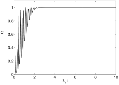
Figure 1: The entanglement in two-mode fields state, where $\lambda_{1}=\lambda_{2}=1$, $\Omega_{1}=\Omega_{2}=20$.

where $+(-)$ correspond to $+(-)$ in Eq.(9). Due to the factor $u$ , the entanglement of state Eq.(9) is different with the state $\frac{1}{N_{\pm}}(|\alpha,\alpha\rangle\pm|-\alpha,-\alpha\rangle)$ xiaoguang VAN even when $\alpha_{1}=\alpha_{2}$. In their case, $\frac{1}{N_{-}}(|\alpha,\alpha\rangle-|-\alpha,-\alpha\rangle)$ is exact one ebit and its entanglement is always 1 while $\frac{1}{N_{+}}(|\alpha,\alpha\rangle+|-\alpha,-\alpha\rangle)$ is maximum state only when $\alpha\rightarrow\infty$. In our case, we find there is little difference between the two state. If we see the state in space $\Re^{\prime}$ our state is exact the same with theirs. When we measure entanglement in space $\Re$, we need to use the form of Eq.(9). Its Concurrence is show in Fig.1 where we choose negative in Eq.(11) and all the parameters are dimensionless. Fig.1 show that Concurrence exhibits a rapid oscillation during a section of starting time which results from the classical field oscillation. After the time evolution section, Concurrence achieves its maximum value 1 and the state is a maximum entangled state. This is because the quantity of $|\alpha_{j}|=\frac{\lambda_{j}t}{2}$ is increased with time $t$ evolution. If the quantity of $\alpha_{j}$ is large enough, $i.e.,$ $\langle\alpha_{j}|-\alpha_{j}\rangle=\exp(-2|\alpha_{j}|^{2})=0$, Concurrence in Eq.(11) will be maximum value 1 and the state of Eq.(9) will be a ebit state. Thus with time evolution, the two-mode field will be a maximum entangled state so that the entanglement in qubit is completely transferred into two-mode fields state.

IV Entanglement retrieval from entangled coherent state to qubits

We have transferred a maximal entanglement to a two-cavity fields completely. Next, we will retrieve the deposit entangled information from two-cavity fields, that is, entanglement transfer from two -cavity fields to atomic state. We assume the two-cavity fields now are entangled coherent state with Eq.(9) form which is produced by the above procedure. Now the two atoms in their ground state $|gg\rangle$ enter into their cavity separately. So, in space $\Re$ the initial state of the system is

$$|\Psi(t)\rangle=\frac{1}{\sqrt{M_{\pm}}}[e^{uti}|\alpha_{1},\alpha_{2}\rangle\pm e^{-uti}|-\alpha_{1},-\alpha_{2}\rangle]|gg\rangle.$$ (12)

where $\alpha_{j}=-\frac{i\lambda_{j}t}{2}$ is a pure complex number which is exact what we deposit during the process of transfer from qubit to fields. The state evolution of the system still obey

$$U(t\prime)=U_{0}^{+}(t^{\prime})e^{-iH_{eff}t^{\prime}}U_{0}(t)=U_{0}^{+}(t^{\prime}-t)e^{-iH_{eff}t^{\prime}}$$ (13)

The evolution will give us state in space $\Re$. We assume $t^{\prime}=t$, which means we will use the same time to retrieve it back when we use time $t$ to deposit it in two-cavity fields. This strategy had been used in lee . The condition unitary evolution operator now is $U(t\prime)=e^{-iH_{eff}t^{\prime}}$. Consider the values of $\alpha_{j}$ is pure complex number, after some calculation, we obtain the state of the system at evolution time $t^{\prime}$ as

$$|\Psi\rangle = [|+,+\rangle(e^{iut}|\alpha_{1}-\frac{i}{2}\lambda_{1}t^{\prime},\alpha_{2}-\frac{i}{2}\lambda_{2}t^{\prime}\rangle$$ (14)

$$\pm e^{-iut}|-\alpha_{1}-\frac{i}{2}\lambda_{1}t^{\prime},-\alpha_{2}-\frac{i}{2}\lambda_{2}t^{\prime}\rangle)$$

$$+|+,-\rangle(e^{iut}|\alpha_{1}-\frac{i}{2}\lambda_{1}t^{\prime},\alpha_{2}+\frac{i}{2}\lambda_{2}t^{\prime}\rangle$$

$$\pm e^{-iut}|-\alpha_{1}-\frac{i}{2}\lambda_{1}t^{\prime},-\alpha_{2}+\frac{i}{2}\lambda_{2}t^{\prime}\rangle)$$

$$+|-,+\rangle(e^{iut}|\alpha_{1}+\frac{i}{2}\lambda_{1}t^{\prime},\alpha_{2}-\frac{i}{2}\lambda_{2}t^{\prime}\rangle$$

$$\pm e^{-iut}|-\alpha_{1}+\frac{i}{2}\lambda_{1}t^{\prime},-\alpha_{2}-\frac{i}{2}\lambda_{2}t^{\prime}\rangle)$$

$$+|-,-\rangle(e^{iut}|\alpha_{1}+\frac{i}{2}\lambda_{1}t^{\prime},\alpha_{2}+\frac{i}{2}\lambda_{2}t^{\prime}\rangle$$

$$\pm e^{-iut}|-\alpha_{1}+\frac{i}{2}\lambda_{1}t^{\prime},-\alpha_{2}+\frac{i}{2}\lambda_{2}t^{\prime}\rangle).$$

Substitute $\alpha_{j}=-\frac{i\lambda_{j}t}{2}$ and $t=t^{\prime}$ into Eq.(14) and rewrite the state as

$$|\Psi\rangle = |+,+\rangle(e^{iut^{\prime}}|-i\lambda_{1}t^{\prime},-i\lambda_{2}t^{\prime}\rangle\pm e^{-iut^{\prime}}|0,0\rangle)$$

$$+|+,-\rangle(e^{iut^{\prime}}|-i\lambda_{1}t^{\prime},0\rangle\pm e^{-iut^{\prime}}|0,i\lambda_{2}t^{\prime}\rangle)$$

$$+|-,+\rangle(e^{iut^{\prime}}|0,-i\lambda_{2}t^{\prime}\rangle\pm e^{-iut^{\prime}}|i\lambda_{1}t^{\prime},0\rangle)$$

$$+|-,-\rangle(e^{iut^{\prime}}|0,0\rangle\pm e^{-iut^{\prime}}|i\lambda_{1}t^{\prime},i\lambda_{2}t^{\prime}\rangle).$$

In order to improve the degree of entanglement transfer to the atoms, postselection measure on the fields is needed. This procedure is similar to what we have detected on the atomic state so as to get a pure two–cavity fields. Here, one can see clearly from Eq.(15) that we will have seven different kinds of cavity fields.

IV.1 Project with $P=|0,0\rangle\langle 0,0|$

If we project the two-cavity fields with $P=|0,0\rangle\langle 0,0|$ $($means we detect the cavity fields as $|0,0\rangle)$, the measure on fields results in the atomic state as

$$|\Psi\rangle=(p_{1}|++\rangle+p_{2}|+-\rangle+p_{3}|-+\rangle+p_{4}|--\rangle)$$ (16)

where

$$p_{1} = e^{-\frac{(\lambda_{1}t^{\prime})^{2}}{2}-\frac{(\lambda_{2}t^{\prime})^{2}}{2}+iut^{\prime}}\pm e^{-iut^{\prime}},$$ (17)

$$p_{2} = e^{-\frac{(\lambda_{1}t^{\prime})^{2}}{2}+iut^{\prime}}\pm e^{-\frac{(\lambda_{2}t^{\prime})^{2}}{2}-iut^{\prime}},$$

$$p_{3} = e^{-\frac{(\lambda_{2}t^{\prime})^{2}}{2}+iut^{\prime}}\pm e^{-\frac{(\lambda_{1}t^{\prime})^{2}}{2}-iut^{\prime}},$$

$$p_{4} = e^{iut^{\prime}}\pm e^{-\frac{(\lambda_{1}t^{\prime})^{2}}{2}-\frac{(\lambda_{2}t^{\prime})^{2}}{2}-iut^{\prime}}.$$

On the bare atomic basis, the state is

$$|\Psi\rangle_{a}=N(A_{gg}|gg\rangle+A_{ge}|ge\rangle+A_{eg}|eg\rangle+A_{ee}|ee\rangle)$$ (18)

where

$$A_{gg} = (p_{1}+p_{4}+p_{2}+p_{3}),$$ (19)

$$A_{ge} = (p_{1}-p_{4}-p_{2}+p_{3}),$$

$$A_{eg} = (p_{1}-p_{4}+p_{2}-p_{3}),$$

$$A_{ee} = (p_{1}+p_{4}-p_{2}-p_{3}),$$

$$N = \frac{1}{\sqrt{A_{gg}^{2}+A_{ge}^{2}+A_{eg}^{2}+A_{ee}^{2}}}.$$

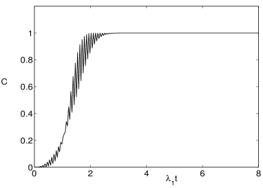
Figure 2: The atomic entanglement change with time, corresponding to positive in Eq.(12). Time here means for different entangled coherent state $\alpha_{j}$ we need use corresponding time to retrive it. The parameters are $\lambda_{1}=\lambda_{2}=1$, $\Omega_{1}=\Omega_{2}=20$.

We still use the concurrence to estimate the entanglement Eq.(18) state. The Concurrence of the state is

$$C{\small=2}N^{2}\sqrt{|A_{ee}A_{gg}|^{2}+|A_{eg}A_{ge}|^{2}-A}$$ (20)

with $A=A_{ee}A_{gg}A_{ge}^{\ast}A_{eg}^{\ast}+A_{ee}^{\ast}A_{gg}^{\ast}A_{ge}A_{eg}$.

The atomic entanglement is shown in Fig.2. One still can see the oscillation resulting from classical field $\Omega_{1}$ and $\Omega_{2}$. Excepting short time section, the entanglement will be maximum value when time $t$ is longer. We can understand it from the analytic expression Eqs. (17)-(19). If $\lambda_{1}=\lambda_{2}$ and large $t$, $p_{2}=p_{3}=0$ and $p_{1}=\pm e^{-iut^{\prime}}$, $p_{4}$ $=e^{iut^{\prime}}$. For positive case, the atomic state is $|\Psi\rangle=\cos ut^{\prime}(|gg\rangle+|ee\rangle)-i\sin ut^{\prime}(|eg\rangle+|ge\rangle)$ which is a always maximal entanglement state. By choosing $ut^{\prime}=n\pi$ or $ut^{\prime}=n\frac{\pi}{2}$, one can obtain Bell state $|\Psi\rangle_{a}=\frac{1}{\sqrt{2}}(|ge\rangle+|eg\rangle)$ or $|\Psi\rangle_{a}=\frac{1}{\sqrt{2}}(|gg\rangle+|ee\rangle)$. Although during short time section, Concurrence is not the maximum value. But it does not mean the entanglement can not be completely transferred. Notice Fig.1 short time section, the amplitude of the fields during this interval is small and the entanglement do not achieve its maximum value. So, we can not retrieve a maximum entanglement if the two-mode fields do not achieve its maximal entanglement. It is easy to see from Eq.(15) that the probability of this projection is 25%.

IV.2 Other Projections $P=|\pm i\lambda_{1}t^{\prime},i\lambda_{2}t^{\prime}\rangle\langle\pm i\lambda_{1}t^{\prime},i\lambda_{2}t^{\prime}|$

Except the projection of $P=|0,0\rangle\langle 0,0|$ , we still have other six projections. If project the two-cavity fields with $P=|-i\lambda_{1}t^{\prime},-i\lambda_{2}t^{\prime}\rangle\langle-i\lambda_{1}t^{\prime},-i\lambda_{2}t^{\prime}|$ $($means we detect the cavity fields as $|-i\lambda_{1}t^{\prime},-i\lambda_{2}t^{\prime}\rangle)$, we have

$$p_{1} = e^{iut^{\prime}}\pm e^{-\frac{(\lambda_{1}t^{\prime})^{2}}{2}-\frac{(\lambda_{2}t^{\prime})^{2}}{2}-iut^{\prime}},$$ (21)

$$p_{2} = e^{-\frac{(\lambda_{2}t^{\prime})^{2}}{2}+iut^{\prime}}\pm e^{-\frac{(\lambda_{1}t^{\prime})^{2}}{2}-2(\lambda_{2}t^{\prime})^{2}-iut^{\prime}},$$

$$p_{3} = e^{-\frac{(\lambda_{1}t^{\prime})^{2}}{2}+iut^{\prime}}\pm e^{-\frac{(\lambda_{2}t^{\prime})^{2}}{2}-2(\lambda_{1}t^{\prime})^{2}-iut^{\prime}},$$

$$p_{4} = e^{\frac{(\lambda_{1}t^{\prime})^{2}}{2}-\frac{(\lambda_{2}t^{\prime})^{2}}{2}+iut^{\prime}}\pm e^{-2(\lambda_{1}t^{\prime})^{2}-2(\lambda_{2}t^{\prime})^{2}-iut^{\prime}}.$$

For this case, the entanglement transferred is shown in Fig. 4 line a. During short evolution time, we can obtain a little entanglement. For large time $t$, $p_{1}=e^{iut}$ and $p_{2}=p_{3}=p_{4}=0$. Thus, $|\Psi\rangle_{a}=\frac{1}{2}(|g\rangle+|e\rangle)(|g\rangle+|e\rangle)$ is a direct product state for positive case. We fail to transfer entanglement. What we get is just to pumping the atomic state from $|g\rangle$ to superposition $|g\rangle+|e\rangle)$ and obtain larger amplitude of the field $i\lambda_{j}t^{\prime}$(first transformation the amplitude is ( $i\lambda_{j}t^{\prime}/2$). If project the two-mode fields with $P=|i\lambda_{1}t^{\prime},i\lambda_{2}t^{\prime}\rangle\langle i\lambda_{1}t^{\prime},i\lambda_{2}t^{\prime}|$, the atomic entanglement behavior is almost the same.

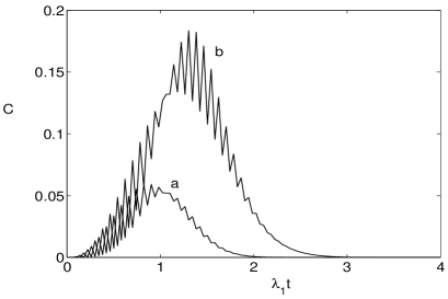
Figure 3: The atomic entanglement change with time, corresponding to positive in Eq.(12). Line a and b correspond to postselection $P=|-i\lambda_{1}t^{\prime},-i\lambda_{2}t^{\prime}\rangle\langle-i\lambda_{1}t^{\prime},-i\lambda_{2}t^{\prime}|$, $P=|-i\lambda_{1}t^{\prime},0\rangle\langle-i\lambda_{1}t^{\prime},0|$, respectively.The parameters are the same with Fig. 2.

With the projection $P=|-i\lambda_{1}t^{\prime},0\rangle\langle-i\lambda_{1}t^{\prime},0|$, we have

$$p_{1} = e^{-\frac{(\lambda_{2}t^{\prime})^{2}}{2}+iut^{\prime}}\pm e^{-\frac{(\lambda_{1}t^{\prime})^{2}}{2}-iut^{\prime}},$$ (22)

$$p_{2} = e^{iut^{\prime}}\pm e^{-\frac{(\lambda_{1}t^{\prime})^{2}}{2}-\frac{(\lambda_{2}t^{\prime})^{2}}{2}-iut^{\prime}},$$

$$p_{3} = e^{-\frac{(\lambda_{1}t^{\prime})^{2}}{2}-\frac{(\lambda_{2}t^{\prime})^{2}}{2}+iut^{\prime}}\pm e^{-2(\lambda_{1}t^{\prime})^{2}-iut^{\prime}},$$

$$p_{4} = e^{-\frac{(\lambda_{1}t^{\prime})^{2}}{2}+iut^{\prime}}\pm e^{-2(\lambda_{1}t^{\prime})^{2}-\frac{(\lambda_{2}t^{\prime})^{2}}{2}-iut^{\prime}}.$$

The transferred entanglement is plotted in Fig.3 line b. At this case, because the cavity mode 2 is projected with vacuum state (inverse the mode), so the entanglement in short time evolution is larger than line a. But, for large time $t$, $p_{2}=e^{iut}$ and $p_{1}=p_{3}=p_{4}=0$. The atomic state is still a product one $|\Psi\rangle_{a}=\frac{1}{2}(|g\rangle+|e\rangle)(|g\rangle-|e\rangle)$. Similarly, we can easy analyze the remaining projection $P=|i\lambda_{1}t^{\prime},0\rangle\langle i\lambda_{1}t^{\prime},0|$ and $P=|0,\pm i\lambda_{1}t^{\prime},0\rangle\langle 0,\pm i\lambda_{1}t^{\prime}|$. Their behaviors are like the case with the projection $P=|-i\lambda_{1}t^{\prime},0\rangle\langle-i\lambda_{1}t^{\prime},0|.$

Up to now, we have analyzed all kinds of projections. We conclude that with the projection $P=|0,0\rangle\langle 0,0|$, we can completely transfer two-cavity entangled coherent state into atomic state.  We can understand it from the reversible property of quantum mechanics. We produce entangled coherent state from atomic entanglement and vacuum cavity mode. Projection with $P=|0,0\rangle\langle 0,0|$ means keeping the two-mode still in vacuum state; in this way the first process is reversed and entanglement will be retrieved back into atomic state. Other projections can not make the two-cavity state in its original one so that entanglement can not be retrieved completely.

V Conclusion

We have considered entanglement transfer between atomic state and two-mode cavity state. By introducing two-mode classical fields, entanglement can be transferred reciprocally. Before our proposal, people try to use Jaynes-Cummings interaction to extract entanglement from continuous-variable system. Due to the impossibility of perfect extraction, Serafini serafini put forward a strategy by using multiple qubits (atomic cloud). We, on the other hand, propose a scheme, by employing two classical fields, which can perfect transfer between atomic state $|\Psi(0)\rangle_{12}=\frac{1}{\sqrt{2}}(|eg\rangle+|ge\rangle)$ and two-cavity entangled coherent state $|\Psi(t)\rangle_{f\pm}=\frac{1}{\sqrt{M_{\pm}}}[e^{uti}|\alpha_{1},\alpha_{2}\rangle\pm e^{-uti}|-\alpha_{1},-\alpha_{2}\rangle]$. Because the entanglement measurement of two-cavity entangled coherent state is very clear and easy, we do not face the hard problem of quantifying entanglement of two-cavity non-Gaussian state. Our entanglement measure quantifying on atomic state and two-cavity state is accurate. Our scheme is also a good example on the transition between microscopic state and macroscopic state.

Acknowledgments:This work was supported by Natural Science Foundation of China under Grant No. 10575017 and Natural Science Foundation of Liaoning Province of China under No. 20031073.

References

- (1) Cirac J I, Zoller P, Kimble H J, and Mabuchi H 1997 Phys. Rev. Lett. 78 3221
- (2) Kraus B and Cirac J I 2004 Phys. Rev. Lett. 92 013602.
- (3) Lee Jinhyoung, Paternostro M, Kim M S and Bose S 2006 Phys. Rev. Lett. 96 080501.
- (4) Hartmann M J, Reuter M E, Plenio M B 2006 New J. Phys. 8 94
- (5) Serafini A, Paternostro M, Kim M S, and Bose S 2006 Phys. Rev. A 73 022312
- (6) Paternostro M, Son W, and Kim M S 2004 Phys. Rev. Lett. 92 197901
- (7) Zou J, Li J G, Shao B, Li J, and Li Q S 2006 Phys. Rev. A 73 042319
- (8) Son W, Kim M S, Lee Jinghyoung, Ahn D 2002 J. of Mod. Opt. 49 1739
- (9) Retzker A, Cirac J I, and Reznik B 2004 Phys. Rev. Lett. 94, 050504().
- (10) Solano E, Agarwal G S and Walther H 2003 Phys. Rev. Lett. 90 027903
- (11) Wang X and Sanders B C 2001 Phys. Rev.A 65 012303
- (12) Wang Xiaoguang 2002 J. Phys. A 35 165
- (13) Hill S and Wootters W K1997 Phys. Rev. Lett. 78 5022
- (14) Wang Xiaoguang 2001 Phys. Rev. A 64 022302
- (15) Enk S J van and Hirota O 2001 Phys. Rev. A 64 022313.