Exact zero-point interaction energy between cylinders

Abstract

We calculate the exact Casimir interaction energy between two perfectly conducting, very long, eccentric cylindrical shells using a mode summation technique. Several limiting cases of the exact formula for the Casimir energy corresponding to this configuration are studied both analytically and numerically. These include concentric cylinders, cylinder-plane, and eccentric cylinders, for small and large separations between the surfaces. For small separations we recover the proximity approximation, while for large separations we find a weak logarithmic decay of the Casimir interaction energy, typical of cylindrical geometries.

1 Introduction

Almost 60 years ago [1], Casimir discovered an interesting macroscopic consequence of the zero point fluctuations of the electromagnetic field: an attractive force between uncharged parallel conducting plates. Since then, the dependence of the Casimir force with the geometry of the conducting surfaces has been the subject of several works [2]. For many years, the only practical way to compute the Casimir energy for non planar configurations was the so called proximity force approximation (PFA) [3]. This approximation is valid for surfaces whose separation is much smaller than typical local curvatures. Due to the high precision experiments performed since 1997 [4], there has been a renewed interest in the geometry dependence of the Casimir force, and in particular in the calculations of the corrections to the proximity approximation.

In the last years there have been a number of attempts to compute the Casimir forces beyond the PFA, using for example semiclassical [5, 6] and optical [7] approximations, and numerical path-integral methods [8]. Large deviations from PFA for corrugated plates have been reported [9], and in recent months the Casimir energy has been computed exactly for several configurations of experimental interest, as the case of a sphere in front of a plane, and a cylinder in front of a plane [10, 11, 12, 13]. As first suggested in [14], the latter configuration is intermediate between the sphere-plane and the plane-plane geometries, and may shed light on the longstanding controversy about thermal corrections to the Casimir force. There is an ongoing experiment to measure precisely the Casimir force for this geometry [15].

The configuration of two eccentric cylinders is of experimental relevance too [14, 16, 17]. Although parallelism is as difficult as for the plane-plane configuration, the fact that the concentric configuration is an unstable equilibrium position opens the possibility of measuring the derivative of the force using null experiments. Up to now, the Casimir interaction energy between two cylindrical shells has been computed semiclassically and exactly in the concentric case [6, 18], and using the proximity approximation in the eccentric situation [14, 16]. In principle, one could consider experimental configurations in which a very thin metallic wire is placed inside a larger hollow cylinder. In this case, a more accurate determination of the Casimir force is needed. The aim of this paper is to describe in detail the derivation of the exact Casimir interaction energy for eccentric cylinders, initially reported by us in [17], and to compute analytically different limiting cases of relevance for Casimir force measurements in this configuration. To this end we will use the mode summation technique combined with the argument theorem in order to write the Casimir energy as a contour integral in the complex plane [19].

The paper is organized as follows. In Section 2 we derive an expression for the Casimir interaction energy for any configuration invariant under translations in one of the spatial dimensions. When properly subtracted, this expression reduces to an integral over the imaginary axis, and is similar to expressions for the Casimir energy derived using path integrals or scattering methods. In Section 3 we derive the exact formula for the interaction energy between eccentric cylinders and we analyze some particular cases of the exact formula. We first show the known results for the concentric case obtained from the exact formulation, and that it is possible to derive the interaction energy for the cylinder-plane configuration in the appropriate limit. In Section 4 we consider the exact formula in the limit of quasi concentric cylinders of arbitrary radii. We discuss two opposite limits of this exact formula: large and small separations between the metallic surfaces. In the first limit, we find that the Casimir energy between a thin wire contained in a hollow cylinder has a weak logarithmic decay as the ratio between the outer and inner radii becomes very large. In the second limit, we recover previous results obtained using PFA for quasi concentric cylinders. Finally, Section 5 contains the conclusions of our work.

2 Casimir energy as a contour integral

The Casimir energy for a system of conducting shells can be written as

$$E_{c}=\frac{1}{2}\sum_{p}(w_{p}-\tilde{w}_{p}),$$ (1)

where $w_{p}$ are the eigenfrequencies of the electromagnetic field satisfying perfect conductor boundary conditions on the surfaces of the conductors, and $\tilde{w}_{p}$ are those corresponding to the reference vacuum (conductors at infinite separation). Throughout this paper we use units $\mathchar 1406\relax=c=1$. The subindex $p$ denotes the set of quantum numbers associated to each eigenfrequency. Introducing a cutoff for high frequency modes $E_{c}(\sigma)={1\over 2}\sum_{p}(e^{-\sigma w_{p}}w_{p}-e^{-\sigma\tilde{w}_{p}}\tilde{w}_{p})$, the Casimir energy $E_{c}$ is the limit of $E_{c}(\sigma)$ as $\sigma\rightarrow 0$. For simplicity we choose an exponential cutoff, although the explicit form is not relevant.

Let us consider a general geometry with translational invariance along the $z-$axis (as for example very long and parallel waveguides of arbitrary sections). The transverse electric (TE) and transverse magnetic (TM) modes can be described in terms of two scalar fields with adequate boundary conditions. In cylindrical coordinates, the modes of each scalar field will be of the form $h_{n,k_{z}}(t,r,\theta,z)=e^{(-iw_{n,k_{z}}t+ik_{z}z)}R_{n}(r,\theta)$, where the eigenfrequencies are $w_{n,k_{z}}=\sqrt{k_{z}^{2}+\lambda^{2}_{n}}$, and $\lambda_{n}$ are the eigenvalues of the two dimensional Laplacian

$$\left(\frac{\partial^{2}}{\partial r^{2}}+\frac{1}{r}\frac{\partial}{\partial r}+\frac{1}{r^{2}}\frac{\partial^{2}}{\partial\theta^{2}}+\lambda_{n}^{2}\right)R_{n}(r,\theta)=0.$$ (2)

The set of quantum numbers $p$ is given by $(n,k_{z})$. For very long cylinders of length $L$ we can replace the sum over $k_{z}$ by an integral. The result is

$$E_{c}(\sigma)={L\over 2}\int_{-\infty}^{\infty}{dk_{z}\over 2\pi}\sum_{n}\left(\sqrt{k_{z}^{2}+\lambda_{n}^{2}}e^{-\sigma\sqrt{k_{z}^{2}+\lambda_{n}^{2}}}-\sqrt{k_{z}^{2}+\tilde{\lambda}_{n}^{2}}e^{-\sigma\sqrt{k_{z}^{2}+\tilde{\lambda}_{n}^{2}}}\right)\;.$$ (3)

From the argument theorem it follows that

$${1\over 2\pi i}\int_{C}\,d\lambda\;\lambda\;e^{-\sigma\lambda}{d\over d\lambda}\ln f(\lambda)=\sum_{i}\lambda_{i}\;e^{-\sigma\lambda_{i}}\;,$$ (4)

where $f(\lambda)$ is an analytic function in the complex $\lambda$ plane within the closed contour ${C}$, with simple zeros at $\lambda_{1},\lambda_{2},\dots$ within ${C}$. We use this result to replace the sum over $n$ in Eq.(3) by a contour integral

$$E_{c}(\sigma)={L\over 4\pi i}\int_{-\infty}^{\infty}{dk_{z}\over 2\pi}\int_{C}d\lambda\sqrt{k_{z}^{2}+\lambda^{2}}e^{-\sigma\sqrt{k_{z}^{2}+\lambda^{2}}}{d\over d\lambda}\ln\left(\frac{F}{F_{\infty}}\right),$$ (5)

where $F$ is a function that vanishes at $\lambda_{n}$ for all $n$ (and $F_{\infty}$ vanishes at $\tilde{\lambda}_{n}$).

Figure 1: Geometrical configuration studied in this paper. Two perfectly conducting eccentric cylinders of radii $a<b$, length $L$, and eccentricity $\epsilon$ interact via the Casimir force. The figure on the right shows the polar coordinates $(r,\theta)$ and $(\rho,\varphi)$ of any point $P$ between the eccentric cylinders used for the determination of the classical eigenvalues for this configuration.

In the rest of this section we will consider the particular configuration of two eccentric cylinders with circular sections of radii $a$ and $b$, respectively. We will denote the eccentricity of the configuration by $\epsilon$ (see Fig. 1). The geometrical dimensionless parameters $\alpha\equiv b/a$ and $\delta\equiv\epsilon/a$ fully characterize the eccentric cylinder configuration. It is worth emphasizing that the results of this section can be trivially extended to more general configurations, as long as they are translationally invariant along one spatial dimension. It is convenient to compute the difference between the energy of the system of two eccentric cylinders and the energy of two isolated cylindrical shells of radii $a$ and $b$,

$$E_{12}(\sigma)=E_{c}(\sigma)-E_{1}(\sigma,a)-E_{1}(\sigma,b)\;,$$ (6)

where

$$E_{1}(\sigma,a)={L\over 4\pi i}\int_{-\infty}^{\infty}{dk_{z}\over 2\pi}\int_{C}d\lambda\sqrt{k_{z}^{2}+\lambda^{2}}e^{-\sigma\sqrt{k_{z}^{2}+\lambda^{2}}}{d\over d\lambda}\ln\left(\frac{F_{1{\rm cyl}}(a)}{F_{1{\rm cyl}}(\infty)}\right)\;.$$ (7)

Here $F_{1{\rm cyl}}(a)$ is a function that vanishes at the eigenfrequencies of an isolated cylindrical shell of radius $a$. Therefore

$$E_{12}(\sigma)={L\over 4\pi i}\int_{-\infty}^{\infty}{dk_{z}\over 2\pi}\int_{C}d\lambda\sqrt{k_{z}^{2}+\lambda^{2}}e^{-\sigma\sqrt{k_{z}^{2}+\lambda^{2}}}{d\over d\lambda}\ln M(\lambda)\;,$$ (8)

where

$$M=\frac{F}{F_{\infty}}\frac{F_{1{\rm cyl}}(\infty)^{2}}{F_{1{\rm cyl}}(a)F_{1{\rm cyl}}(b)}\;.$$ (9)

Figure 2: Contour for the integration in the complex plane.

To proceed we must choose a contour for the integration in the complex plane. In order to compute $E_{c}(\sigma),E_{1}(\sigma,a)$, and $E_{1}(\sigma,b)$ separately, an adequate contour is a circular segment ${C}_{\Gamma}$ and two straight line segments forming an angle $\phi$ and $\pi-\phi$ with respect to the imaginary axis (see Fig. 2). The nonzero angle $\phi$ is needed to show that the contribution of ${C}_{\Gamma}$ vanishes in the limit $\Gamma\rightarrow\infty$ when $\sigma>0$. For the rest of the contour, the divergences in $E_{c}(\sigma)$ are cancelled out by those of $E_{1}(\sigma,a)$ and $E_{1}(\sigma,b)$, as in the case of concentric cylinders [6]. Therefore, in order to compute $E_{12}(\sigma)$ we can set $\phi=0$ and $\sigma=0$, and the contour integral reduces to an integral on the imaginary axis. We find

$$E_{12}=-{L\over 2\pi}\int_{-\infty}^{\infty}{dk_{z}\over 2\pi}~{}{\rm Im}\left\{\int_{0}^{\infty}dy\sqrt{k_{z}^{2}-y^{2}}{d\over dy}\ln M(iy)\right\}\;.$$ (10)

As we will see, $M(iy)$ is a real function - hence, the integral over $y$ in Eq. (10) is restricted to $y>k_{z}$. After some straightforward steps one can re-write this equation as

$$E_{12}={L\over 4\pi}\int_{0}^{\infty}dy\ y\ln M(iy)\;.$$ (11)

As we have already mentioned, a similar expression can be derived for conductors of arbitrary shape, as long as there is translational invariance along the $z$-axis. It is worth noting that the structure of this expression is similar to the ones derived recently for the cylinder-plane geometry using path integrals [11, 12], and for the sphere-plane geometry using the Krein formula [10].

3 The exact formula

In this section we derive the exact formula for the Casimir energy between eccentric cylinders. We proceed in two steps: we first find the function $F$ with zeroes at the eigenfrequencies for the geometric configuration. Then we obtain an explicit expression for the function $M$, which involves a definition of the Casimir energy as a difference between the energy of the actual configuration and a configuration with very large and separated conductors.

3.1 The classical eigenvalues

The solution of the Helmholtz equation in the annular region between eccentric cylinders has been considered in the framework of classical electrodynamics, fluid dynamics, and reactor physics, among others [20, 21]. The eigenvalues have been computed using different approaches, as for instance conformal transformations that map the eccentric annulus onto a concentric one. As the two dimensional Helmholtz equation is not conformally invariant, the transformed equation has coordinate dependent coefficients and has to be solved numerically [22]. As is well known, it is very difficult to compute the Casimir energy from the numerical eigenfrequencies. It is more efficient to use the procedure outlined in Section 2, that only needs a function $F$ with zeroes at the eigenvalues. Although for the eccentric annulus this function has been previously found in the literature [20, 21], for the benefit of the reader we include here a derivation of this result.

The electromagnetic field inside an eccentric waveguide can be described in terms of TM and TE modes. The TM modes are characterized by a vanishing $z$ component of the magnetic field, $B_{z}=0$. The other components of the electromagnetic field can be derived from the $z$ component of the electric field, $E_{z}(r,\theta,z,t)=E(r,\theta)e^{-i\omega t+izk_{z}}$, with

$$E(r,\theta)=\sum_{m}\left[A_{m}J_{m}(\lambda r)+B_{m}N_{m}(\lambda r)\right]e^{im\theta},$$ (12)

where $w^{2}=k_{z}^{2}+\lambda^{2}$, and $(r,\theta)$ are polar coordinates with origin at the center of the outer cylinder (see Fig. 1). One can also describe the $z$ component of the electric field using polar coordinates $(\rho,\varphi)$ with origin at the center of the inner cylinder (see Fig. 1),

$$\bar{E}(\rho,\varphi)=\sum_{n}\left[\bar{A}_{n}J_{n}(\lambda\rho)+\bar{B}_{n}N_{n}(\lambda\rho)\right]e^{in\varphi}\,.$$ (13)

The perfect conductor boundary conditions imply that the $z$ component of the electric field must vanish on the cylindrical shells

$$A_{m}J_{m}(\lambda b)+B_{m}N_{m}(\lambda b) = 0,$$

$$\bar{A}_{n}J_{n}(\lambda a)+\bar{B}_{n}N_{n}(\lambda a) = 0\,\,,$$ (14)

i.e., the functions $E$ and $\bar{E}$ satisfy Dirichlet boundary conditions on the surfaces. The coefficients of the series in Eqs.(12) and (13) can be related to one another using the addition theorem for Bessel functions

$$e^{im\varphi}{\cal C}_{m}(\lambda\rho)=\sum_{p}e^{ip\theta}{\cal C}_{p}(\lambda r)J_{p-m}(\lambda\epsilon)\,\,,$$ (15)

where ${\cal C}_{m}$ denotes either $J_{m}$ or $N_{m}$. Indeed, as at any point $P$ in the annulus region one must have $E(P)=\bar{E}(P)$, it is possible to show that

$$\bar{A}_{n} = \sum_{m}A_{m}J_{n-m}(\lambda\epsilon),$$

$$\bar{B}_{n} = \sum_{m}B_{m}J_{n-m}(\lambda\epsilon).$$ (16)

Combining Eqs. (14) and (16) one obtains the linear, homogeneous system of equations

$$\sum_{m}A_{m}\left[\frac{J_{n}(\lambda a)}{N_{n}(\lambda a)}-\frac{J_{m}(\lambda b)}{N_{m}(\lambda b)}\right]J_{n-m}(\lambda\epsilon)=0.$$ (17)

The solution of this linear system of equations is non trivial only if ${\rm det}[Q^{\rm TM}_{mn}]=0$, where

$$Q^{\rm TM}_{mn}(a,b,\epsilon)=\left[J_{n}(\lambda a)N_{m}(\lambda b)-J_{m}(\lambda b)N_{n}(\lambda a)\right]J_{n-m}(\lambda\epsilon)\,\,.$$ (18)

This equation defines the allowed values for $\lambda$, and therefore defines the eigenfrequencies of the TM modes.

The TE modes can be treated in the same fashion. For these modes the $z$ component of the electric field vanishes in the annulus region, $E_{z}=0$. The perfect conductor boundary conditions imply that the normal component of the magnetic field should vanish on the conducting shells, so now we must impose Neumann boundary conditions on the surfaces. The eigenvalues $\lambda$ for the TE modes are the solutions of ${\rm det}[Q^{\rm TE}_{mn}]=0$, where

$$Q^{\rm TE}_{mn}(a,b,\epsilon)=\left[J^{\prime}_{n}(\lambda a)N^{\prime}_{m}(\lambda b)-J^{\prime}_{m}(\lambda b)N^{\prime}_{n}(\lambda a)\right]J_{n-m}(\lambda\epsilon).$$ (19)

In the concentric limit $\epsilon=0$ we have $J_{n-m}(0)=\delta_{nm}$, the two matrices $Q^{\rm TE}_{mn}$ and $Q^{\rm TM}_{mn}$ become diagonal, and the equations for the eigenvalues are those of the concentric case [6]. In what follows we will use these matrices to define the function $M$ that enters in Eq.(11).

3.2 The function $M$

Roughly speaking, the function $M$ that determines the Casimir energy through Eq.(11) is the ratio of the function associated to the actual geometric configuration and the one associated to a configuration in which the conducting surfaces are very far away from each other. As the last configuration is not univocally defined, we will use this freedom to choose a particular one that simplifies the calculation. It turns to be convenient to subtract a configuration of two cylinders with very large (and very different) radii, but with the same eccentricity as that of the configuration of interest.

We start considering the Dirichlet modes. To compute $F_{1{\rm cyl}}(a)$ in Eq.(9) we note that the eigenfrequencies $\lambda$ for the geometry of a single cylinder of radius $a$ surrounded by a larger one of radius $R$ are defined by the equations

$$J_{n}(\lambda a)=0\,,$$

$$J_{n}(\lambda a)N_{n}(\lambda R)-J_{n}(\lambda R)N_{n}(\lambda a)=0\;.$$ (20)

The first equation defines the eigenfrequencies in the region $r<a$ and the second one gives the eigenfrequencies of the modes in the region $a<r<R$. $F_{1{\rm cyl}}(a)$ is the product of these two relations for all values of $n$, evaluated on the imaginary axis ($\lambda=iy\equiv i\beta/a$). Namely,

$$F_{1{\rm cyl}}(a) = \prod_{n}J_{n}(\lambda a)[J_{n}(\lambda a)N_{n}(\lambda R)-J_{n}(\lambda R)N_{n}(\lambda a)]$$ (21)

$$\equiv J(a){\rm det}[Q^{\rm TM}(a,R,0)]\;,$$

where we have introduced the notation $J(a)\equiv\prod_{n}J_{n}(\lambda a)$ to simplify the formulas below. The function $F_{1{\rm cyl}}(\infty)$ has the same expression, but replacing $a$ by $R_{1}$, with $R_{1}$ very large but smaller than $R$. Using the asymptotic expansion of the modified Bessel functions it is easy to prove that $F_{1{\rm cyl}}(a)/F_{1{\rm cyl}}(\infty)\simeq 2\beta I_{n}(\beta)K_{n}(\beta)R_{1}/a$. The functions $F$ and $F_{\infty}$ in Eq.(9) are given by

$$F = J(a){\rm det}[Q^{\rm TM}(a,b,\epsilon)]{\rm det}[Q^{\rm TM}(b,R,0)]$$ (22)

$$= \frac{J(a)}{J(b)}{\rm det}[Q^{\rm TM}(a,b,\epsilon)]F_{1{\rm cyl}}(b),$$

$$F_{\infty} = \frac{J(R_{1})}{J(R_{2})}{\rm det}[Q^{\rm TM}(R_{1},R_{2},\epsilon)]F_{1{\rm cyl}}(\infty),$$ (23)

where $R_{1}<R_{2}<R$. As we already stressed, in order to define $F_{\infty}$ we consider a configuration of two eccentric cylinders of large radii $R_{1}<R_{2}$ and with the same eccentricity $\epsilon$ of the original configuration. Evaluating the determinant in Eq.(22) on the imaginary axis one obtains

$${\rm det}[Q^{\rm TM}(a,b,\epsilon)] = {\rm det}\left[\frac{2}{\pi}I_{n-m}\left(\beta\frac{\epsilon}{a}\right)[K_{n}(\beta)I_{m}(\alpha\beta)\right.$$ (24)

$$- \left.(-1)^{m+n}I_{n}(\beta)K_{m}(\alpha\beta)]\right].$$

Using again the asymptotic expansions of the Bessel functions one gets ${\rm det}[Q^{\rm TM}(R_{1},R_{2},\epsilon)]\propto aI_{n-m}(\beta\epsilon/a)\frac{e^{\beta(R_{2}-R_{1})/a}}{2\sqrt{R_{1}R_{2}}\beta}$. The equations above can be combined to obtain

$$M^{\rm TM}(\beta) = \,{\rm det}\,\left[I_{n-m}(\beta\epsilon/a)\frac{I_{m}(\alpha\beta)}{I_{n}(\alpha\beta)}\left[1-(-1)^{m+n}\frac{I_{n}(\beta)K_{m}(\alpha\beta)}{K_{n}(\beta)I_{m}(\alpha\beta)}\right]\right]$$ (25)

$$\times {\rm det}\,I_{nm}^{-1}\left(\beta\frac{\epsilon}{a}\right),$$

where $I_{nm}^{-1}(\beta\epsilon/a)$ denotes the inverse matrix of $I_{n-m}(\beta\epsilon/a)$ and $\alpha\equiv b/a$. Computing explicitly the determinant one can show that the factor $I_{m}(\alpha\beta)/I_{n}(\alpha\beta)$ cancels out. Moreover, writing $M^{\rm TM}$ as a single determinant we get

$$M^{\rm TM}(\beta)={\rm det}[\delta_{np}-A_{np}^{\rm TM}],$$ (26)

with

$$A_{np}^{\rm TM}=(-1)^{n}\frac{I_{n}(\beta)}{K_{n}(\beta)}\sum_{m}(-1)^{m}\frac{K_{m}(\alpha\beta)}{I_{m}(\alpha\beta)}I_{n-m}\left(\beta\frac{\epsilon}{a}\right)I_{mp}^{-1}\left(\beta\frac{\epsilon}{a}\right).$$ (27)

The addition theorem for the modified Bessel functions, ${\cal C}_{m}(u\pm v)=\sum_{p}{\cal C}_{m\mp p}(u)J_{p}(v)$ [23], implies that $I_{mp}^{-1}(\beta\epsilon/a)=(-1)^{m-p}I_{m-p}(\beta\epsilon/a)$. Finally, the elements of the matrix $A^{\rm TM}$ read

$$A_{np}^{\rm TM}=\frac{I_{n}(\beta)}{K_{n}(\beta)}\sum_{m}\frac{K_{m}(\alpha\beta)}{I_{m}(\alpha\beta)}I_{n-m}\left(\beta\frac{\epsilon}{a}\right)I_{p-m}\left(\beta\frac{\epsilon}{a}\right),$$ (28)

where we omitted a global factor $(-1)^{n+p}$ because it does not contribute to the determinant.

The analysis for the TE modes is straightforward, the main difference being that $Q^{\rm TE}(a,b,\epsilon)$ contains derivatives of those Bessel functions that do not depend on the eccentricity. Therefore, following similar steps it is possible to show that

$$M^{\rm TE}(\beta)={\rm det}[\delta_{np}-A_{np}^{\rm TE}],$$ (29)

where

$$A_{np}^{\rm TE}=\frac{I^{\prime}_{n}(\beta)}{K^{\prime}_{n}(\beta)}\sum_{m}\frac{K^{\prime}_{m}(\alpha\beta)}{I^{\prime}_{m}(\alpha\beta)}I_{n-m}\left(\beta\frac{\epsilon}{a}\right)I_{p-m}\left(\beta\frac{\epsilon}{a}\right).$$ (30)

The function $M$ for the electromagnetic field is the product $M=M^{\rm TE}M^{\rm TM}$, and therefore the interaction energy is the sum of the TE and TM contributions

$$E_{12} = \frac{L}{4\pi a^{2}}\int_{0}^{\infty}d\beta\,\beta\,\ln M(\beta)=\frac{L}{4\pi a^{2}}\int_{0}^{\infty}d\beta\,\beta\,\ln M^{\rm TE}(\beta)$$ (31)

$$+ \frac{L}{4\pi a^{2}}\int_{0}^{\infty}d\beta\,\beta\,\ln M^{\rm TM}(\beta)=E^{{\rm TE}}+E^{{\rm TM}}.$$

In order to calculate the exact Casimir interaction energy one needs to perform a numerical evaluation of the determinants. We find that as $\alpha$ approaches smaller values, larger matrices are needed for ensuring convergence. Moreover, for increasing values of the eccentricity $\epsilon$ it is necessary to include more terms in the series defining the coefficients $A_{np}^{\rm TE,TM}$. In Fig. 3 we plot the interaction energy difference $\Delta E=E_{12}-E_{12}^{\rm cc}$ between the eccentric ($E_{12}$) and the concentric ($E_{12}^{\rm cc}$) configurations as a function of $\alpha$ for different values of $\delta$. As we will show below, these numerical results interpolate between the PFA and the asymptotic behavior for large $\alpha$. Fig. 4 shows the complementary information, with the Casimir energy as a function of $\delta$ for various values of $\alpha$, showing explicitly that the concentric equilibrium position is unstable.

Figure 3: Exact Casimir interaction energy difference $|\Delta E|$ between the eccentric and concentric configurations as a function of $\alpha=b/a$ for different values of $\delta=\epsilon/a$. Here $\Delta E=E_{12}-E_{12}^{\rm cc}$. Energies are measured in units of $L/4\pi a^{2}$. These results interpolate between the $(\alpha-1)^{-5}$ behavior for $\alpha\rightarrow 1$, and the $(\alpha^{4}\log\alpha)^{-1}$ behavior for $\alpha\gg 1$.

Figure 4: Exact Casimir interaction energy difference $\Delta E$ between the eccentric and concentric configurations as a function of $\delta=\epsilon/a$ for different values of $\alpha=b/a$. Energies are measured in units of $L/4\pi a^{2}$. The maximum at $\delta=0$ shows the instability of the concentric equilibrium position.

3.3 Concentric Cylinders

The exact Casimir interaction between concentric cylinders [6] can be obtained as a particular case of the exact formulas (28), (30). In the concentric limit $\epsilon=0$, the matrices that appear in the definition of $M^{\rm TE}$ and $M^{\rm TM}$ become diagonal and the Casimir energy reads [6]

$$E_{12}^{\rm cc}={L\over 4\pi a^{2}}\int_{0}^{\infty}d\beta\ \beta\ln M^{\rm cc}(\beta),$$ (32)

where

$$M^{\rm cc}(\beta)=\prod_{n}\left[1-{I_{n}(\beta)K_{n}(\alpha\beta)\over I_{n}(\alpha\beta)K_{n}(\beta)}\right]\left[1-{I^{\prime}_{n}(\beta)K^{\prime}_{n}(\alpha\beta)\over I^{\prime}_{n}(\alpha\beta)K^{\prime}_{n}(\beta)}\right].$$ (33)

The first factor corresponds to Dirichlet (TM) modes and the second one to Neumann (TE) modes.

The proximity limit $\alpha-1\ll 1$ has already been analyzed for the concentric case [6]. In order to compute the concentric Casimir interaction energy in this limit it was necessary to perform the summation over all values of $n$. As expected, the resulting value is equal to the one obtained via the proximity approximation, namely

$$E_{12,{\rm PFA}}^{\rm TE,cc}=E_{12,{\rm PFA}}^{\rm TM,cc}=\frac{1}{2}E_{12,{\rm PFA}}^{\rm EM,cc}=-\frac{\pi^{3}L}{720a^{2}}\;\frac{1}{(\alpha-1)^{3}}.$$ (34)

Here $E^{\rm EM,cc}$ denotes the full electromagnetic Casimir interaction energy in the concentric configuration.

In the large $\alpha$ limit one can show that only the $n=0$ term contributes to the interaction energy

$$E_{12}^{\rm cc}\approx{L\over 4\pi b^{2}}\int_{0}^{\infty}dx\ x\left[\ln\left(1-\frac{I_{0}(\frac{x}{\alpha})K_{0}(x)}{I_{0}(x)K_{0}(\frac{x}{\alpha})}\right)+\ln\left(1-\frac{I^{\prime}_{0}(\frac{x}{\alpha})K^{\prime}_{0}(x)}{I^{\prime}_{0}(x)K^{\prime}_{0}(\frac{x}{\alpha})}\right)\right].$$ (35)

Using the small argument behavior of the Bessel functions it is easy to prove that, in the limit $\alpha\gg 1$, the TM mode contribution dominates, giving

$$E_{12}^{\rm cc}\approx-{L\over 4\pi b^{2}\ln\alpha}\int_{0}^{\infty}dx\ x\frac{K_{0}(x)}{I_{0}(x)}\approx-{1.26L\over 8\pi b^{2}\ln\alpha}.$$ (36)

Note that the modulus of the energy decreases logarithmically with $\alpha$. Fig. 5 depicts the exact Casimir interaction energy between concentric cylinders as a function of $\alpha$, for values that interpolate between the above mentioned limiting cases.

It is worth noticing that, while for small values of $\alpha$ both TM and TE modes contribute with the same weight to the interaction energy, the TM modes dominate in the large $\alpha$ limit.

Figure 5: Modulus of the Casimir interaction energy in the concentric case as a function of $\alpha=b/a$. Energies are measured in units of $L/4\pi a^{2}$. These results interpolate between the $(\alpha-1)^{-3}$ behavior for $\alpha\rightarrow 1$, and the $(\alpha^{2}\log\alpha)^{-1}$ behavior for $\alpha\gg 1$.

3.4 A cylinder in front of a plane

It is interesting to see how the Casimir energy for the cylinder-plane configuration is contained as a particular case of the exact formula derived in Section 3.2. To do that let us consider a cylinder of radius $a$ in front of an infinite plane, and let us denote by $H$ the distance between the center of the cylinder and the plane. The eccentric cylinders formula should reproduce the cylinder-plane Casimir energy in the limit $b,\epsilon\rightarrow\infty$ keeping $H=b-\epsilon$ fixed (see Fig. 1).

We note that for $x\gg h>1$ the ratio of Bessel functions appearing in Eq.(28) can be approximated by

$$\frac{I_{m-n}(x)I_{m-p}(x)}{I_{m}(x+h)}\simeq I_{m-n-p}(x-h).$$ (37)

This is trivially true for fixed $m$ and large values of $x$, as can be seen from the large argument expansion of the Bessel functions. Moreover, using the uniform expansion of the Bessel functions, it can be shown that Eq.(37) is also valid in the large $m$ limit, for all values of $x$. Therefore we approximate

$$\sum_{m}\frac{K_{m}(x+h)}{I_{m}(x+h)}I_{m-n}(x)I_{m-p}(x) \simeq \sum_{m}K_{m}(x+h)I_{m-p-n}(x-h)$$ (38)

$$= K_{n+p}(2h),$$

where in the last equality we used the addition theorem of Bessel functions. Inserting this result (with $x\equiv\beta\epsilon/a$ and $h\equiv\beta H/a$) in Eq.(28) we get

$$A_{np}^{\rm TM}\simeq\frac{I_{n}(\beta)}{K_{n}(\beta)}K_{n+p}(2\beta H/a)\equiv A_{np}^{\rm TM,c-p},$$ (39)

which coincides with the known result for the Dirichlet matrix elements for the cylinder-plane geometry [11, 12]. The TE modes can be analyzed in the same fashion. Using that for large $x$

$$\frac{K^{\prime}_{m}(x)I_{m}(x)}{K_{m}(x)I^{\prime}_{m}(x)}\simeq-1\,\,,$$ (40)

one can prove that

$$\sum_{m}\frac{K^{\prime}_{m}(x+h)}{I^{\prime}_{m}(x+h)}I_{m-n}(x)I_{m-p}(x) \simeq -\sum_{m}K_{m}(x+h)I_{m-p-n}(x-h)$$ (41)

$$= -K_{n+p}(2h).$$

Therefore, from Eq.(30) we obtain

$$A_{np}^{\rm TE}\simeq-\frac{I^{\prime}_{n}(\beta)}{K^{\prime}_{n}(\beta)}K_{n+p}(2\beta H/a)\equiv A_{np}^{\rm TE,c-p},$$ (42)

which is the result for the TE modes in the cylinder-plane geometry [11, 12].

4 Quasi-concentric cylinders

We will now consider a situation in which the eccentricity of the configuration is much smaller than the radius of the inner cylinder, i.e., $\delta=\epsilon/a\ll 1$. As discussed in [14] this configuration may be relevant for performing null experiments to look for extra gravitational forces. Note that we do not assume that the radius of the inner and outer cylinder are similar, so the proximity approximation is in general not valid for this configuration.

As described in the previous section, when $\epsilon=0$ the matrix defining the eigenfrequencies is diagonal. When considering a small non-vanishing eccentricity, the behavior of the Bessel functions for small arguments $I_{m-n}(\beta\delta)\sim(\beta\delta)^{n-m}$ suggests that one only needs to use matrix elements near the diagonal. Using this idea, we will approximate the Casimir interaction energy by keeping only terms proportional to $I_{0},I_{1}$ and $I_{1}^{2}$. In this approximation, the matrices $\delta_{np}-A_{np}^{\rm TM}$ and $\delta_{np}-A_{np}^{\rm TE}$ become tridiagonal matrices, and the $\epsilon-$dependent part of the Casimir energy will be quadratic in the eccentricity.

We will describe in detail the case of the Dirichlet modes; the treatment of Neumann modes is similar. To order $O(\delta^{2})$ the only non-vanishing elements of the matrix $A_{np}^{\rm TM}$ are

$$A_{n,n}^{\rm TM} \simeq \frac{I_{n}(\beta)}{K_{n}(\beta)}\left[\frac{K_{n}(\alpha\beta)}{I_{n}(\alpha\beta)}I_{0}^{2}(\delta\beta)+\frac{K_{n-1}(\alpha\beta)}{I_{n-1}(\alpha\beta)}I_{1}^{2}(\delta\beta)+\frac{K_{n+1}(\alpha\beta)}{I_{n+1}(\alpha\beta)}I_{1}^{2}(\delta\beta)\right],$$

$$A_{n,n+1}^{\rm TM} \simeq \frac{I_{n}(\beta)}{K_{n}(\beta)}\left[\frac{K_{n}(\alpha\beta)}{I_{n}(\alpha\beta)}+\frac{K_{n+1}(\alpha\beta)}{I_{n+1}(\alpha\beta)}\right]I_{0}(\delta\beta)I_{1}(\delta\beta),$$

$$A_{n+1,n}^{\rm TM} \simeq \frac{I_{n+1}(\beta)}{K_{n+1}(\beta)}\left[\frac{K_{n}(\alpha\beta)}{I_{n}(\alpha\beta)}+\frac{K_{n+1}(\alpha\beta)}{I_{n+1}(\alpha\beta)}\right]I_{0}(\delta\beta)I_{1}(\delta\beta).$$ (43)

We split the matrix $A^{\rm TM}$ into three terms, $A^{\rm TM}={\cal D}^{\rm TM,cc}+{\cal D}^{\rm TM}+{\cal N}^{\rm TM}$, where ${\cal D}^{\rm TM,cc}$ is the diagonal matrix corresponding to the concentric case, ${\cal D}^{\rm TM}$ the diagonal part of the matrix that depends on $\delta$, and ${\cal N}^{\rm TM}$ is the non-diagonal part of the matrix. The non-vanishing matrix elements are

$${\cal D}_{n,n}^{\rm TM,cc} = \frac{I_{n}(\beta)}{K_{n}(\beta)}\frac{K_{n}(\alpha\beta)}{I_{n}(\alpha\beta)},$$

$${\cal D}_{n,n}^{\rm TM} = A_{n,n}^{\rm TM}-{\cal D}_{n,n}^{\rm TM,cc},$$

$${\cal N}_{n,n+1}^{\rm TM} = A_{n,n+1}^{\rm TM},\quad{\cal N}_{n+1,n}^{\rm TM}=A_{n+1,n}^{\rm TM}.$$ (44)

Note that although ${\cal D}^{\rm TM}=O(\delta^{2})$ and ${\cal N}^{\rm TM}=O(\delta)$, both give quadratic contributions to the determinant. Up to this order we have

$$\ln{\rm det}\,[1-A^{\rm TM}] \simeq \ln{\rm det}\,[1-{\cal D}^{\rm TM,cc}]+\ln{\rm det}\left[1-\frac{{\cal D}^{\rm TM}}{1-{\cal D}^{\rm TM,cc}}\right]$$ (45)

$$+ \ln{\rm det}\left[1-\frac{{\cal N}^{\rm TM}}{1-{\cal D}^{\rm TM,cc}}\right].$$

The first term is associated to the interaction energy between concentric cylinders $E_{12}^{\rm cc}$, studied in Section 3.3, and being $\delta$-independent does not contribute to the force between eccentric cylinders. The second term can be easily evaluated

$$\ln{\rm det}\left[1-\frac{{\cal D}^{\rm TM}}{1-{\cal D}^{\rm TM,cc}}\right]\simeq\ln\left(1-{\rm tr}\,\frac{{\cal D}^{\rm TM}}{1-{\cal D}^{\rm TM,cc}}\right)\simeq-\sum_{n}\frac{{\cal D}^{\rm TM}_{n,n}}{1-{\cal D}_{n,n}^{\rm TM,cc}}.$$ (46)

To compute the last term in Eq.(45) we use that the determinant of an arbitrary tridiagonal matrix $T$ of dimension $p$ can be calculated using the recursive relation ${\rm det}[T_{\{p\}}]=T_{p,p}{\rm det}[T_{\{p-1\}}]-T_{p,p-1}T_{p-1,p}\,{\rm det}[T_{\{p-2\}}]$, where $T_{\{k\}}$ denotes the submatrix formed by the first $k$ rows and columns of $T$. Up to quadratic order in $\delta$ we obtain

$$\ln{\rm det}\left[1-\frac{{\cal N}^{\rm TM}}{1-{\cal D}^{\rm TM,cc}}\right] \simeq \ln\left(1-\sum_{n}\frac{A_{n,n+1}^{\rm TM}\;A_{n+1,n}^{\rm TM}}{(1-{\cal D}_{n,n}^{\rm TM,cc})(1-{\cal D}_{n+1,n+1}^{\rm TM,cc})}\right)$$ (47)

$$\simeq -\sum_{n}\frac{A_{n,n+1}^{\rm TM}\;A_{n+1,n}^{\rm TM}}{(1-{\cal D}_{n,n}^{\rm TM,cc})(1-{\cal D}_{n+1,n+1}^{\rm TM,cc})}.$$

Putting all together, the TM part of the Casimir interaction energy between quasi-concentric cylinders can be written as

$$E_{12}^{\rm TM}=E_{12}^{{\rm TM,cc}}-\frac{L\epsilon^{2}}{4\pi a^{4}}\sum_{n}\int_{0}^{\infty}d\beta\;\beta^{3}\frac{1}{1-{\cal D}^{\rm TM,cc}_{n,n}}\left[{\cal D}^{\rm TM}_{n}+\frac{{\cal N}^{\rm TM}_{n}}{1-{\cal D}^{\rm TM,cc}_{n+1,n+1}}\right].$$ (48)

Here

$${\cal D}^{\rm TM}_{n} \equiv \frac{{\cal D}^{\rm TM,cc}_{n,n}}{2}+\frac{I_{n}(\beta)}{4K_{n}(\beta)}\left[\frac{K_{n-1}(\alpha\beta)}{I_{n-1}(\alpha\beta)}+\frac{K_{n+1}(\alpha\beta)}{I_{n+1}(\alpha\beta)}\right],$$

$${\cal N}^{\rm TM}_{n} \equiv \frac{I_{n}(\beta)I_{n+1}(\beta)}{4K_{n}(\beta)K_{n+1}(\beta)}\left[\frac{K_{n}(\alpha\beta)}{I_{n}(\alpha\beta)}+\frac{K_{n+1}(\alpha\beta)}{I_{n+1}(\alpha\beta)}\right]^{2}.$$ (49)

The corresponding formulas for the TE modes can be obtained from these ones by replacing the Bessel functions by their derivatives with respect to the argument.

The expression for the Casimir energy for quasi-concentric cylinders derived in this section is far simpler than the exact formulas Eqs.(28), (30). It is very useful for the analytical and numerical evaluation of the Casimir energy in the different limiting cases we will study below: the large distance limit ($a\ll b$), for which one obtains a logarithmic decay of the energy, and the small distance limit ($a\simeq b$), where the proximity approximation holds. The first case is very simple to handle because the energy is dominated by the lowest modes, while the second case is much more involved.

4.1 Large distances: logarithmic decay

When the ratio of the outer and the inner radii $\alpha=b/a$ is much larger than one, the exact Casimir energy is dominated by the lowest term $n=0$ in the summation. Moreover, it can be shown that the contribution of the Dirichlet modes is much larger than the contribution of the Neumann modes. Therefore, from Eq.(31) we get, in the limit $\alpha\rightarrow\infty$,

$$E_{12}^{\infty}\simeq{L\over 4\pi a^{2}}\int_{0}^{\infty}d\beta\;\beta\ln(1-A_{00}^{\rm TM}(\beta))\simeq-{L\over 4\pi a^{2}\alpha^{2}}\int_{0}^{\infty}dx\;x\;A_{00}^{\rm TM}\left(\frac{x}{\alpha}\right),$$ (50)

where

$$A_{00}^{\rm TM}\left(\frac{x}{\alpha}\right)\simeq\frac{I_{0}(\frac{x}{\alpha})}{K_{0}(\frac{x}{\alpha})}\left[\frac{K_{0}(x)}{I_{0}(x)}I_{0}^{2}\left(\frac{\delta x}{\alpha}\right)+2\frac{K_{1}(x)}{I_{1}(x)}I_{1}^{2}\left(\frac{\delta x}{\alpha}\right)\right]\,.$$ (51)

Using the small argument expansion of the Bessel functions it is easy to see that

$$A_{00}^{\rm TM}\left(\frac{x}{\alpha}\right)\simeq\frac{1}{\ln\alpha}\left[\frac{K_{0}(x)}{I_{0}(x)}+\frac{\delta^{2}x^{2}}{2\alpha^{2}}\left(\frac{K_{0}(x)}{I_{0}(x)}+\frac{K_{1}(x)}{I_{1}(x)}\right)\right].$$ (52)

In this expression, valid when $a,\epsilon\ll b$, we kept the leading terms proportional to $(\alpha^{2}\ln\alpha)^{-1}$ and only the subleading terms that depend on the eccentricity. Inserting Eq.(52) into Eq.(50) and computing numerically the integrals we find

$$E_{12}^{\infty}\simeq-{L\over 8\pi b^{2}\ln\alpha}\left(1.26+3.33\frac{\epsilon^{2}}{b^{2}}\right),$$ (53)

where the first term is the concentric contribution $E_{12}^{\infty,{\rm cc}}$ derived before (see Eq.(36)). It is worth to note that Eqs. (52) and (53) have been derived under the assumption $\ln\alpha\gg 1$, and therefore are valid for extremely large values of $\alpha$. For intermediate values $\alpha\gg 1,\ln\alpha=O(1)$, the interaction energy is also dominated by the Dirichlet $n=0$ term. The final result is still of the form given in Eq.(53), with numerical coefficients that depend logarithmically on $\alpha$. In Fig. 6 we plot the ratio between the exact Casimir interaction energy difference $\Delta E\equiv E_{12}-E_{12}^{\rm cc}$ and its asymptotic expression $\Delta E_{\infty}\equiv E_{12}^{\infty}-E_{12}^{\infty,{\rm cc}}$ as a function of $\alpha$. As mentioned, extremely large values of $\alpha$ are needed in order for the ratio of energies to asymptotically approach 1. From Eq.(53) we see that the force between cylinders in the limit $a,\epsilon\ll b$ is proportional to $L\epsilon/b^{4}\ln(b/a)$. The weak logarithmic dependence on the ratio $b/a$ is characteristic of the cylindrical geometry (see also [11, 12]), and it is also found in the electrostatic counterpart of the Casimir energy, that we briefly analyze next.

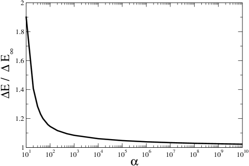
Figure 6: Ratio of the exact $\Delta E$ and asymptotic $\Delta E_{\infty}$ Casimir energy differences in the limit of small eccentricity $\epsilon\ll a$. In the $\alpha\rightarrow\infty$ limit, the Casimir energy difference between eccentric and concentric configurations decays logarithmically as $(\alpha^{4}\log\alpha)^{-1}$.

The electrostatic capacity for the system of two eccentric cylinders is given by

$$C=\frac{2\pi\epsilon_{0}L}{\ln[Y+\sqrt{Y^{2}-1}]},$$ (54)

where $Y=(a^{2}+b^{2}-\epsilon^{2})/2ab$, and $\epsilon_{0}$ is the permittivity of vacuum. Therefore, the electrostatic force between cylinders kept at a fixed potential difference $V$ is

$$F_{\rm elec}=\frac{\epsilon}{ab}\frac{\pi\epsilon_{0}V^{2}L}{\sqrt{Y^{2}-1}\ln^{2}[Y+\sqrt{Y^{2}-1}]}.$$ (55)

In the quasi-concentric case we can set $\epsilon=0$ in the definition of $Y$. In the large $\alpha$ limit we get

$$F_{\rm elec}\simeq\frac{L\epsilon}{b^{2}\log^{2}\left(\frac{b}{a}\right)}.$$ (56)

Just as in the Casimir case, in the limit $a\ll b$ the Coulomb force decays logarithmically with the ratio $a/b$.

4.2 Small distances: the proximity approximation

The proximity limit for concentric cylinders has been reviewed in Sec. 3.3; the case of a cylinder in front of a plane has been considered in detail in [12]. In this section we extend these results to the case of quasi-concentric cylinders.

We will concentrate on calculating the Casimir interaction energy difference $\Delta E\equiv E_{12}-E_{12}^{\rm cc}$ between the eccentric ($E_{12}$) and the concentric ($E_{12}^{\rm cc}$) configurations. As the small distance limit is dominated by the large-$n$ modes, the key point in the derivation of the PFA from the exact expression of the Casimir energy is the use of the uniform approximation for the Bessel functions. In the large $n$ limit, and to leading order in $\alpha-1$ one has

$$\frac{I_{n}(\beta)}{K_{n}(\beta)}\frac{K_{n}(\alpha\beta)}{I_{n}(\alpha\beta)} \simeq e^{-2n(\alpha-1)h(x)},$$

$$\frac{I_{n}(\beta)}{K_{n}(\beta)}\frac{K_{n\pm 1}(\alpha\beta)}{I_{n\pm 1}(\alpha\beta)} \simeq e^{-2n(\alpha-1)h(x)}\left[\frac{1+h(x)}{x}\right]^{\pm 2},$$ (57)

where $\beta=nx$ and $h(x)=\sqrt{1+x^{2}}$. Inserting these approximations in Eq.(49) we get

$${\cal D}^{\rm TM}_{n}(nx)=\frac{e^{-2n(\alpha-1)h(x)}}{2}\left[1+\frac{1}{2}\left(\frac{1+h(x)}{x}\right)^{2}+\frac{1}{2}\left(\frac{1+h(x)}{x}\right)^{-2}\right].$$ (58)

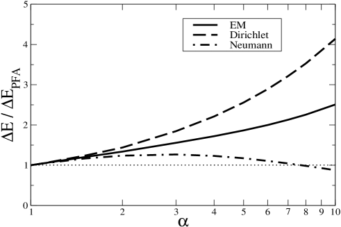
Figure 7: Ratio of the exact and PFA Casimir interaction energy differences $\Delta E=E_{12}-E_{12}^{\rm cc}$ between eccentric ($E_{12}$) and concentric ($E_{12}^{\rm cc}$) cylinders in the limit of small eccentricity $\epsilon\ll a$. The curve EM denotes the full electromagnetic Casimir energy.

The contribution to the interaction energy coming from the diagonal part of the matrix can be written as (see Eq.(48))

$$\Delta E_{\cal D}^{\rm TM}=-\frac{L\delta^{2}}{2\pi a^{2}}\sum_{n,k\geq 1}\int_{0}^{\infty}d\beta\;\beta^{3}\;{\cal D}^{\rm TM}_{n}({\cal D}_{n,n}^{\rm TM,cc})^{k-1},$$ (59)

where we replaced the sum over all integers $n$ by twice the sum over the positive integers (the term $n=0$ gives a subleading contribution for small $\alpha-1$). Inserting the uniform expansions into Eq.(59) and changing variables in the integral we obtain

$$\Delta E^{\rm TM}_{\cal D} = -\frac{L\delta^{2}}{4\pi a^{2}}\sum_{n,k\geq 1}n^{4}\int_{0}^{\infty}dx\;x^{3}e^{-2n(\alpha-1)h(x)k}$$ (60)

$$\times\left[1+\frac{1}{2}\left(\frac{1+h(x)}{x}\right)^{2}+\frac{1}{2}\left(\frac{1+h(x)}{x}\right)^{-2}\right].$$

To leading order in $\alpha-1$ the sum over $n$ gives $\sum_{n}n^{4}e^{-2n(\alpha-1)h(x)}\simeq 24/[2h(x)(\alpha-1)k]^{5}$. Next we perform first the sum over $k$ and then the integral over $x$. We get

$$\Delta E^{\rm TM}_{\cal D}=-\frac{3}{8}\frac{L\delta^{2}\zeta(5)}{\pi a^{2}(\alpha-1)^{5}},$$ (61)

where $\zeta(x)$ is the Riemann zeta function.

The evaluation of the non diagonal contribution to the Casimir energy can be done using similar steps, starting from Eq.(47). In the proximity limit, we can approximate ${\cal D}_{n+1,n+1}^{\rm TM,cc}$ by ${\cal D}_{n,n}^{\rm TM,cc}$ in the denominator of that equation. Therefore, using Eq.(48)we write the non diagonal contribution to the energy as

$$\Delta E^{\rm TM}_{\cal ND}\simeq-\frac{L\delta^{2}}{2\pi a^{2}}\int_{0}^{\infty}d\beta\;\beta^{3}\sum_{n,k\geq 1}{\cal N}^{\rm TM}_{n}\;k\;({\cal D}_{n,n}^{\rm TM,cc})^{k-1}.$$ (62)

Now we use the uniform expansion for the Bessel functions in Eq.(49) to obtain

$${\cal N}^{\rm TM}_{n} \simeq \frac{e^{-4n(\alpha-1)h(x)}}{2}$$ (63)

$$\times\left[1+\frac{1}{2}\left(\frac{1+h(x)}{x}\right)^{2}+\frac{1}{2}\left(\frac{1+h(x)}{x}\right)^{-2}\right].$$

Replacing Eq.(63) into Eq.(62) we get

$$\Delta E^{\rm TM}_{\cal ND} = -\frac{L\delta^{2}}{8\pi a^{2}}\sum_{n,k\geq 1}n^{4}\int_{0}^{\infty}dx\;x^{3}\;e^{-2n(k+1)(\alpha-1)h(x)}\;k$$ (64)

$$\times\left[2+\left(\frac{1+h(x)}{x}\right)^{2}+\left(\frac{1+h(x)}{x}\right)^{-2}\right].$$

As before, we first compute the sum over $n$, and expand the result to leading order in $\alpha-1$. The sum over $k$ can be calculated using that $\sum_{k\geq 1}\frac{k}{(k+1)^{5}}=\zeta(4)-\zeta(5)$. Finally, we compute analytically the remaining integrals to get

$$\Delta E^{\rm TM}_{\cal ND}=-\frac{3}{8}\frac{L\delta^{2}}{\pi a^{2}(\alpha-1)^{5}}(\zeta(4)-\zeta(5)).$$ (65)

The contribution of the Dirichlet modes to the Casimir interaction energy in the limit $\alpha\rightarrow 1$ is therefore

$$\Delta E^{\rm TM}=\Delta E^{\rm TM}_{\cal D}+\Delta E^{\rm TM}_{\cal ND}=-\frac{L\delta^{2}}{a^{2}(\alpha-1)^{5}}\frac{\pi^{3}}{240}.$$ (66)

It can be shown that the contribution of the TE modes to the interaction energy in the short distance limit is equal to that of the TM modes, as expected from the parallel plate configuration. Indeed, the uniform expansion for the ratio of Bessel functions is equal to the expansion for the derivatives, i.e.,

$$\frac{I_{n}^{\prime}(\beta)}{K_{n}^{\prime}(\beta)}\frac{K_{n}^{\prime}(\alpha\beta)}{I_{n}^{\prime}(\alpha\beta)} \simeq e^{-2n(\alpha-1)h(x)},$$

$$\frac{I_{n}^{\prime}(\beta)}{K_{n}^{\prime}(\beta)}\frac{K_{n\pm 1}^{\prime}(\alpha\beta)}{I_{n\pm 1}^{\prime}(\alpha\beta)} \simeq e^{-2n(\alpha-1)h(x)}\left[\frac{1+h(x)}{x}\right]^{\pm 2},$$ (67)

and therefore all calculations can be repeated without changes.

The final result for the Casimir interaction energy difference in the small distance approximation is

$$\Delta E_{\rm PFA}^{\rm TE}=\Delta E_{\rm PFA}^{\rm TM}=\frac{1}{2}\Delta E_{\rm PFA}^{\rm EM}=-\frac{\pi^{3}L\epsilon^{2}}{240a^{4}(\alpha-1)^{5}},$$ (68)

where $\Delta E^{\rm EM}$ denotes the full electromagnetic Casimir energy difference between eccentric and concentric configurations. Fig. 7 depicts the ratio of the exact Casimir energy difference $\Delta E$ and the PFA limit for the almost concentric cylinders configuration. As evident from the figure, PFA agrees with the exact result at a few percent level only for $\alpha$ close to unity, and then it noticeably departs from the PFA prediction. The resulting PFA expression for the attractive Casimir force between quasi-concentric cylinders reads

$$F^{\rm PFA}=\frac{\pi^{3}}{60}\frac{\epsilon L}{a^{4}(\alpha-1)^{5}},$$ (69)

that reproduces the result previously obtained in [14].

5 Conclusions

We have derived an exact formula for the Casimir interaction energy between eccentric cylinders using a mode summation technique. This formula is written as an integral of the determinant of an infinite dimensional matrix, and it reproduces as a particular case the interaction energy between concentric cylinders, and as a limiting case the energy in the cylinder-plane geometry. In the quasi-concentric case, the infinite dimensional matrix becomes tridiagonal, and hence much easier to deal with than the exact formula when performing analytic and numerical calculations. We have carried out the numerical evaluation of the Casimir interaction energy using both the exact and tridiagonal formulas, and studied different limiting cases of relevance for Casimir force measurements.

The large and small distance limits were analyzed. In the former case, the Casimir energy is dominated by the lowest modes, and shows a weak logarithmic decay, typical of cylindrical geometries. In the latter case, the Casimir energy is dominated by the highest modes, and the exact formula reproduces the proximity approximation. We found that the first order correction ($\alpha-1\ll 1$) to PFA for the quasi-concentric cylinders has the form $\Delta E/\Delta E_{\rm PFA}=1+s(\alpha-1)+O((\alpha-1)^{2})$, where the coefficient of the linear curvature correction is positive, $s>0$, both for TE and TM modes. This contrasts with the first order corrections to PFA in the cylinder-plane configuration, where the linear curvature correction to TM modes is positive, while the one for TE modes is negative [12].

The exact Casimir force computed in this paper, in particular for the quasi-concentric configuration, offers a qualitatively different approach for implementing new experiments to measure the Casimir force and to search for extra-gravitational forces in the micrometer and nanometer scales, since it opens the possibility of measuring the derivative of the force using (Cavendish-like) null experiments.

References

References

- [1] H.B.G. Casimir, Proc. K. Ned. Akad. Wet. B 51, 793 (1948).
- [2] G. Plunien, B. Müller, and W. Greiner, Phys. Rep. 134, 87 (1986); P. Milonni, The Quantum Vacuum (Academic Press, San Diego, 1994); V. M. Mostepanenko and N. N. Trunov, The Casimir Effect and its Applications (Clarendon, London, 1997); M. Bordag, The Casimir Effect 50 Years Later (World Scientific, Singapore, 1999); M. Bordag, U. Mohideen, and V. M. Mostepanenko, Phys. Rep. 353, 1 (2001); K. A. Milton, The Casimir Effect: Physical Manifestations of the Zero-Point Energy (World Scientific, Singapore, 2001); S. Reynaud et al., C. R. Acad. Sci. Paris IV-2, 1287 (2001); K. A. Milton, J. Phys. A: Math. Gen. 37, R209 (2004); S.K. Lamoreaux, Rep. Prog. Phys. 68, 201 (2005).
- [3] B.V. Derjaguin and I.I. Ibrikosova, Sov. Phys. JETTP 3, 819 (1957); B.V. Derjaguin, Sci. Am. 203, 47 (1960); J. Blocki, J. Randrup, W.J. Swiatecki, and C.F. Tsang, Ann. Phys. 105, 427 (1977).
- [4] S.K. Lamoreaux, Phys. Rev. Lett. 78, 5 (1997); U. Mohideen and A. Roy, Phys. Rev. Lett. 81, 4549 (1998); B.W. Harris, F. Chen, and U. Mohideen, Phys. Rev. A 62, 052109 (2000); T. Ederth, Phys. Rev. A 62, 062104 (2000); H.B. Chan, V.A. Aksyuk, R.N. Kleiman, D.J. Bishop, and F. Capasso, Science 291, 1941 (2001); H. B. Chan, V.A. Aksyuk, R.N. Kleiman, D.J. Bishop, and F. Capasso, Phys. Rev. Lett. 87, 211801 (2001); G. Bressi, G. Carugno, R. Onofrio, and G. Ruoso, Phys. Rev. Lett. 88, 041804 (2002); D. Iannuzzi, I. Gelfand, M. Lisanti, and F. Capasso, Proc. Nat. Ac. Sci. USA 101, 4019 (2004); R.S. Decca, D. López, E. Fischbach, and D.E. Krause, Phys. Rev. Lett. 91, 050402 (2003); R.S. Decca et al., Phys. Rev. Lett. 94, 240401 (2005); R.S. Decca et al., Annals of Physics 318, 37 (2005).
- [5] M. Schaden and L. Spruch, Phys. Rev. A 58, 935 (1998).
- [6] F.D. Mazzitelli, M.J. Sánchez, N.N. Scoccola, and J. von Stecher, Phys. Rev. A 67, 013807 (2003).
- [7] R. L. Jaffe and A. Scardicchio, Phys. Rev. Lett. 92, 070402 (2004)
- [8] H. Gies, K. Langfeld, and L. Moyaerts, J. High Energy Phys. 6, 18 (2003).
- [9] C. Genet, A. Lambrecht, Paulo A. Maia Neto, and S. Reynaud, Europhys. Lett. 62, 484 (2003); R.B. Rodrigues, Paulo A. Maia Neto, A. Lambrecht, and S. Reynaud, Phys. Rev. Lett. 96, 100402 (2006).
- [10] A. Bulgac, P. Magierski, and A. Wirzba, Phys. Rev. D 73, 025007 (2006).
- [11] T. Emig, R.J. Jaffe, M. Kardar, and A. Scardicchio, Phys. Rev. Lett. 96, 080403 (2006).
- [12] M. Bordag, Phys. Rev. D 73, 125018 (2006).
- [13] H. Gies and K. Klingmuller, Phys. Rev. Lett. 96, 220401 (2006).
- [14] D.A.R. Dalvit, F.C. Lombardo, F.D. Mazzitelli, and R. Onofrio, Europhys. Lett. 68, 517 (2004).
- [15] M. Brown-Hayes, D.A.R. Dalvit, F.D. Mazzitelli, W.J. Kim, and R. Onofrio, Phys. Rev. A 72, 052102 (2005).
- [16] F.D. Mazzitelli, in Quantum Field Theory Under the Influence of External Conditions, K.A. Milton (editor), Rinton Press, Princeton (2004).
- [17] D.A.R. Dalvit, F.C. Lombardo, F.D. Mazzitelli, and R. Onofrio, Phys. Rev. A 74, 020101(R) (2006).
- [18] A.A. Saharian, ICTP Report IC/2000/14, arXiv:hep-th/0002239; A.A. Saharian and A.S. Tarloyan, arXiv:hep-th/0603144.
- [19] See, for example, V.V. Nesterenko and I.G. Pirozhenko, Phys. Rev D 57, 1284 (1998).
- [20] G.S. Singh and L.S. Kothari, J. Math. Phys. 25, 810 (1984).
- [21] J.A. Balseiro, Revista de la Union Matemática Argentina, v. XIV, 118 (1950).
- [22] M.J. Hine, J. Sound Vib. 15, 295 (1971).
- [23] This is a particular case of Eq.(15), valid for .