Strong Violations of Bell-type Inequalities for Path-Entangled Number States

Abstract

We show that nonlocal correlation experiments on the two spatially separated modes of a maximally path-entangled number state may be performed. They lead to a violation of a Clauser-Horne Bell inequality for any finite photon number $N$. We also present an analytical expression for the two-mode Wigner function of a maximally path-entangled number state and investigate a Clauser-Horne-Shimony-Holt Bell inequality for such a state. We test other Bell-type inequalities. Some are violated by a constant amount for any $N$.

I Introduction

Maximally path-entangled number states of the form

$$|\Psi\rangle=\frac{1}{\sqrt{2}}(|N\rangle_{a}|0\rangle_{b}+e^{i\varphi}|0\rangle_{a}|N\rangle_{b})\,,$$ (1)

(often referred as N00N states) have important applications to quantum imaging Boto , metrology Lee ; Migdall , and sensing Lee2 . Characterizing their quantum mechanical properties is therefore a valuable task for improving upon the above applications. Entanglement is the most profound property of quantum mechanical systems. N00N states are non-separable states and hence are entangled. But do they also show nonlocal behavior when we perform a correlation experiment on their modes? The amount of nonlocality demonstrated by a Bell-type experiment provides an operational definition of entanglement (for a review of Bell inequalities and experiments see, e.g., Genovese . It distinguishes between the class of states that are entangled but admit a local hidden variable model and those which do not and so may be called EPR correlated Werner .

Several publications Reed address the question of whether the N00N states are EPR correlated for the case $N=1$. Gisin and Peres have shown that it is possible to find pairs of observables, whose correlations violate a Bell’s inequality for any nonfactorable pure state of two quantum systems Gisin . This result was later extended to states of more than two systems by Popescu and Rohrlich Popescu . Recent experiments Lvovsky ; Bellini have reported strong evidence that N00N states violate a Bell’s inequality for $N=1$, leaving open the question as to what experiments might show EPR correlations for $N>1$.

We propose a specific experiment that shows that N00N states are EPR correlated for any finite $N$. We investigate two measurement schemes using the unbalanced homodyne detection scheme described in Banaszek and compare the results. The correlation functions we calculate can be related to two well-known phase space distributions: the two-mode $Q$ function and the two-mode Wigner function. Banaszek and Wódkiewicz first pointed out the operational definition of the $Q$ and Wigner function Banaszek . We modify this approach and calculate the distribution functions for the N00N states entirely from these phase space distributions, and thereby construct a Clauser-Horne and a Clauser-Horne-Shimony-Holt Bell inequality. In section IV we also test other Bell-type inequalities not commonly used so far in quantum optical experiments.

The above Bell-tests may be performed in an unbalanced homodyne detection scheme as given, for example, in Ref.Banaszek and shown in Fig. 1.

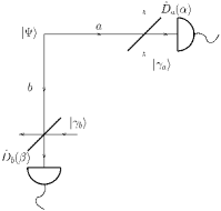
Figure 1: Unbalanced homodyne detection scheme for a Bell experiment with N00N states. Here $|\Psi\rangle=\frac{1}{\sqrt{2}}(|N\rangle_{a}|0\rangle_{b}-|0\rangle_{a}|N\rangle_{b})$ and $a$ and $b$ label the modes.

For simplicity we choose $\varphi=\pi$ for the states in Eq. (1).

It is now understood that the introduction of a reference frame is required in any Bell test Bartlet and one should consider the field modes as entangled rather than the photons vanEnk ; vanEnk_2 . In the number basis, a shared local oscillator acts as the required reference frame. The beam splitters in this approach are assumed to operate in the limit where the transmittivity $T\rightarrow 1$. We further assume that a strong coherent state $|\gamma\rangle$, where $|\gamma|\rightarrow\infty$, is incident on one of the two input ports. The beam splitter then acts as the displacement operator $\hat{D}(\gamma\sqrt{1-T})$ on the second input port Wiseman ; Banaszek_2 ; Wallentowitz . We introduce complex parameters $\alpha=\gamma_{a}\sqrt{1-T}$ and $\beta=\gamma_{b}\sqrt{1-T}$. The phase-space parameterization with respect to these parameters is then analogous to a correlation experiment with polarized light and different relative polarizer settings where the nonlocality of polarization entangled states such as $|\Psi\rangle=(|H\rangle_{a}|V\rangle_{b}-|V\rangle_{a}|H\rangle_{b})/\sqrt{2}$ is well established.

II Bell experiment with on-off detection scheme

In the first experimental setup we consider a simple nonnumber resolving photon-detection scheme. In the case of the homodyne detection scheme under consideration, the local positive operator valued measure (POVM) is defined by $\hat{Q}(\alpha)+\hat{P}(\alpha)=\hat{{\bf 1}}$ with,

$$\hat{Q}(\alpha) = \hat{D}(\alpha)|0\rangle\langle 0|\hat{D}^{\dagger}(\alpha)\,,$$ (2)

$$\hat{P}(\alpha) = \hat{D}(\alpha)\sum_{n=1}^{\infty}|n\rangle\langle n|\hat{D}^{\dagger}(\alpha)\,.$$ (3)

We assume lossless detectors for our investigation. The expectation value of $\hat{Q}(\alpha)$ tells us the probability that no photons are present, depending on the phase and amplitude of the local oscillator. The expectation value of $\hat{P}(\alpha)$ gives the probability of counting one or more photons, while not distinguishing between one or more photons. So we simply assign a 1 to a detector click and a 0 otherwise, giving us a binary result. We label the two modes of the N00N state by $a$ and $b$. The corresponding measurement operators for a correlated measurement of the displaced vacuum can be written as $\hat{Q}_{a}(\alpha)\otimes\hat{Q}_{b}(\beta)$. The expectation value for the state $|\Psi\rangle$ is given by

$$Q_{ab}(\alpha,\beta)=\langle\Psi|\hat{Q}_{a}(\alpha)\otimes\hat{Q}_{b}(\beta)|\Psi\rangle=|\langle\alpha,\beta|\Psi\rangle|^{2}\,.$$ (4)

The above expression is the two-mode $Q$ function of the N00N state up to a factor $1/\pi^{2}$, and the result is given by

$$Q_{ab}(\alpha,\beta)=\frac{1}{2N!}e^{-(|\alpha|^{2}+|\beta|^{2})}|\alpha^{N}-\beta^{N}|^{2}\,.$$ (5)

To obtain the probabilities for the individual measurements we calculate

$$Q_{a}(\alpha) = \langle\Psi|\hat{Q}_{a}(\alpha)\otimes\hat{{\bf 1}}_{b}|\Psi\rangle=\frac{1}{2}{e}^{-|\alpha|^{2}}\left(\frac{|\alpha|^{2N}}{N!}+1\right),$$ (6)

$$Q_{b}(\beta) = \langle\Psi|\hat{{\bf 1}}_{a}\otimes\hat{Q}_{b}(\beta)|\Psi\rangle=\frac{1}{2}{e}^{-|\beta|^{2}}\left(\frac{|\beta|^{2N}}{N!}+1\right).$$ (7)

Using the completeness relation $\hat{P}(\alpha)=\hat{{\bf 1}}-\hat{Q}(\alpha)$, we obtain the probabilities for the correlated and single detector counts — $P_{a}(\alpha)=1-Q_{a}(\alpha)$, $P_{b}(\beta)=1-Q_{b}(\beta)$, and $P_{ab}(\alpha,\beta)=1-Q_{a}(\alpha)-Q_{b}(\beta)+Q_{ab}(\alpha,\beta)$ — in terms of the $Q$ functions. We build from these the Clauser-Horne combination (CH) Clauser-Horne , which for a local hidden variable model admits the inequality,

$$-1 \leq P_{ab}(\alpha,\beta)-P_{ab}(\alpha,\beta^{\prime})+P_{ab}(\alpha^{\prime},\beta)+P_{ab}(\alpha^{\prime},\beta^{\prime})$$ (8)

$$-P_{a}(\alpha^{\prime})-P_{b}(\beta)\leq 0\,.$$

If this inequality is violated it follows that N00N states contain nonlocal correlations, i.e., EPR correlations. In order to attain such a violation, we minimize the function $CH=P_{ab}(\alpha,\beta)-P_{ab}(\alpha,\beta^{\prime})+P_{ab}(\alpha^{\prime},\beta)+P_{ab}(\alpha^{\prime},\beta^{\prime})-P_{a}(\alpha^{\prime})-P_{b}(\beta)$ for a given $N$ over the parameter space spanned by $\alpha$, $\alpha^{\prime}$, $\beta$, and $\beta^{\prime}$. The violation of the Clauser-Horne combination for the N00N states with $N=1,\ldots,4$ is shown in Fig. 2.

Figure 2: Violation of the Clauser-Horne Bell inequality as a function of $N$.

The results show a decrease in the amount of violation with $N$. The maximal violation is obtained for $N=1$. For $N\geq 3$ the violation is so reduced that it would be increasingly hard to observe experimentally. If we increase the precision of our numerical method, we observe that for large $N$ the minimum of the CH combination, in fact, never hits the classical bound of $-1$ exactly, i.e., there is a violation of the inequality for any finite $N$, which can be shown as follows. Let $N$ be finite and odd. We choose $\alpha^{\prime}=\beta=0$ and $\alpha=-\beta^{\prime}$, then the CH combination reduces to $CH=1/N!\,|\alpha|^{2N}e^{-|\alpha|^{2}}(1-2e^{-|\alpha|^{2}})-1$. For any $0<|\alpha|^{2}<\ln 2$, we obtain $CH<-1$. For even $N$ the same proof holds except that we need to choose $\alpha=\beta^{\prime}$ instead.

The Bell measurement presented leads to a decrease of the amount of violation with $N$. This decrease with $N$ is due to the specific way the reference frame is introduced in terms of the local displacement operators $\hat{D}(\alpha)$ and $\hat{D}(\beta)$ for the correlation measurement. The scheme is based on measuring the overlap of coherent states with the modes of the N00N state. The elements contained in Eq. (4) are of the form $\langle N,0|\alpha,\beta\rangle$ and $\langle 0,N|\alpha,\beta\rangle$. In order to maximize those products we would need $\alpha$ to take, at the same time, the values $|\alpha|^{2}=N$ and $|\alpha|^{2}=0$. Since the ‘distance’ of $N$ to the vacuum becomes larger with $N$, the correlated overlap is reduced. This may explain the decrease in the amount of violation observed.

We can also display some correlations by plotting the marginals of the $Q$ function in Eq. (4). We therefore decompose the dimensionless complex local oscillator amplitudes in the set of real variables $x,y,u,v$, i.e., $\alpha=x+i\,y$, $\beta=u+i\,v$, and obtain $Q_{\mathrm{m}}(y,v)=\int_{-\infty}^{\infty}\int_{-\infty}^{\infty}Q_{ab}(x,y,u,v)\,dx\,du$. These probability densities are displayed in Fig. 3, 4, and 5, for $N=1,2,3$. We see that the distributions for $N=2,3$ have a higher symmetry than for $N=1$.

Figure 3: The marginal $Q$ function $Q_{\mathrm{m}}(y,v)$ for $N=1$.

Figure 4: The marginal $Q$ function $Q_{\mathrm{m}}(y,v)$ for $N=2$.

Figure 5: The marginal $Q$ function $Q_{\mathrm{m}}(y,v)$ for $N=3$.

The linear correlation coefficient $r=\mathrm{cov}(y,v)/(\Delta y\Delta v)$, where $\mathrm{cov}(y,v)=\int_{-\infty}^{\infty}\int_{-\infty}^{\infty}(y-\bar{y})(v-\bar{v})Q_{\mathrm{m}}(y,v)\,\,dy\,\,dv$, vanishes for all $N>1$, although we see from the pictures that the two phase space variables are statistically dependent. This is an indication of nonlinear correlations between the two phase space variables. Note that the measurement described by the operators in Eq. (2) and Eq. (3) requires only non-number resolving photon counters and may therefore be performed with current detector technology. In the next section we consider a correlated parity measurement on the modes and investigate the amount of violation in this scheme.

III Bell test with parity measurement

An operational definition of the two-mode Wigner function for the N00N state is given in terms of a correlated parity measurement Banaszek . The measurements can be described by the following POVM operators:

$$\hat{\Pi}^{+}(\alpha) = \hat{D}(\alpha)\sum_{k=0}^{\infty}|2k\rangle\langle 2k|\hat{D}^{\dagger}(\alpha)\,,$$ (9)

$$\hat{\Pi}^{-}(\alpha) = \hat{D}(\alpha)\sum_{k=0}^{\infty}|2k+1\rangle\langle 2k+1|\hat{D}^{\dagger}(\alpha)\,.$$ (10)

The corresponding operator for the correlated measurement of the parity on mode $a$ and $b$ may be defined as:

$$\hat{\Pi}(\alpha,\beta)=\left(\hat{\Pi}_{a}^{(+)}(\alpha)-\hat{\Pi}_{a}^{(-)}(\alpha)\right)\otimes\left(\hat{\Pi}_{b}^{(+)}(\beta)-\hat{\Pi}_{b}^{(-)}(\beta)\right).$$

The outcome of the measurements are either $+1$ or $-1$. It may be noted that this operator can be rewritten as

$$\hat{\Pi}(\alpha,\beta)=\hat{D}_{a}(\alpha)\hat{D}_{b}(\beta)(-1)^{\hat{n}_{a}+\hat{n}_{b}}\hat{D}_{a}^{\dagger}(\alpha)\hat{D}_{b}^{\dagger}(\beta)\,,$$ (11)

and is equivalent to the operator for the Wigner function in Royer ; Moya (up to a factor $4/\pi^{2}$). We note that the operator in Eq. (11) is essentially a product of operators for mode $a$ and $b$:

$$\hat{\Pi}(\alpha,\beta)=\hat{D}_{a}(\alpha)(-1)^{\hat{n}_{a}}\hat{D}_{a}^{\dagger}(\alpha)\hat{D}_{b}(\beta)(-1)^{\hat{n}_{b}}\hat{D}_{b}^{\dagger}(\beta)\,.$$ (12)

Using this property the expectation value of Eq. (12) for the N00N state can be expressed as a function of two Laguerre polynomials and an interference term,

$$\Pi(\alpha,\beta)=\langle\Psi|\hat{\Pi}(\alpha,\beta)|\Psi\rangle=$$ (13)

$$\frac{1}{2}e^{-2|\alpha|^{2}-2|\beta|^{2}}\large[(-1)^{N}(L_{N}(4|\alpha|^{2})+L_{N}(4|\beta|^{2}))$$

$$-\frac{2^{2N}}{N!}({\alpha^{*}}^{N}\beta^{N}+\alpha^{N}{\beta^{*}}^{N})\large]\,,$$

where $L_{N}(x)$ is the Laguerre polynomial Stegun . The two-mode Wigner function is obtained from $W(\alpha,\beta)=\Pi(\alpha,\beta)4/\pi^{2}$. By building the CHSH clauser inequality defined by

$$-2\leq\Pi(\alpha,\beta)+\Pi(\alpha^{\prime},\beta)+\Pi(\alpha,\beta^{\prime})-\Pi(\alpha^{\prime},\beta^{\prime})\leq 2\,,$$ (14)

we determine how this Bell inequality is violated as a function of $N$. A minimization procedure in the parameter space $\alpha$, $\alpha^{\prime}$, $\beta$, and $\beta^{\prime}$ as a function of $N$ is carried out with a numerical routine to investigate the amount of violation. We see that the correlated parity measurement leads to a violation of the CHSH Bell inequality for $N=1$, and that states with larger $N$ do not violate the inequality.

The Wigner function may also be used to understand this behavior. We therefore calculate the marginals of the Wigner function by integrating over two of the variables, where we use the same decomposition of the dimensionless complex local oscillator amplitudes $\alpha=x+i\,y$ and $\alpha=u+i\,v$, and obtain $W_{\mathrm{m}}(y,v)=\int_{-\infty}^{\infty}\int_{-\infty}^{\infty}W(x,y,u,v)dx\,du$. The function $W_{\mathrm{m}}(y,v)$ is positive definite and can be interpreted as the probability density for the remaining variables.

Figure 6: The marginal Wigner function $W_{\mathrm{m}}(y,v)$ for $N=1$.

Figure 7: The marginal Wigner function $W_{\mathrm{m}}(y,v)$ for $N=2$.

Figure 8: The marginal Wigner function $W_{\mathrm{m}}(y,v)$ for $N=3$.

From the density plots in Fig. 6, 7, and 8 we see that the probability densities become more symmetric the larger $N$ becomes, similar to the previous case for the marginals of the $Q$ function, but the interference structures are much more pronounced than for the $Q$ function. Here we also obtain a vanishing correlation coefficient $r$ for all $N>1$, from which we can infer that a nonlinear correlation measure is necessary to describe these correlations.

We conclude from the results of the first section that a set of parameters can always be found which violate the CH inequality in Eq. (8). Therefore N00N states show EPR correlations for any finite $N$. The presented setup is not yet optimal but might be promising for demonstrating EPR correlations of N00N states with low photon numbers $N$ experimentally. Although, the requirements for the overall detection efficiency for a loophole-free test of the CHSH Bell inequality would be very large, i.e., $96\%$ for $N=1$ Bellini .

In the following section we are going to show that the test of other Bell-type inequalities leads to a different result.

IV More Bell-type inequalities

So far we have used the CH and the CHSH Bell inequalities defined in Eq. (8) and Eq. (14). Other Bell inequalities might be more suitable for a Bell test for a nonlocal experiment with N00N states. The CH Bell inequality is a specific inequality for four correlated events, where at most two are intersected at the same time. Pitowsky Pitowsky derived all the Bell-type inequalities for three and four correlated events:

$$0\leq p_{i}-p_{ij}-p_{ik}+p_{jk}\,,$$ (15)

$$p_{i}+p_{j}+p_{k}-p_{ij}-p_{ik}-p_{jk}\leq 1\,,$$ (16)

$$-1\leq p_{ik}-p_{j\ell}+p_{i\ell}+p_{jk}-p_{i}-p_{k}\leq 0\,,$$ (17)

for any different $i,j,k,\ell$. Eq. (17) is the CH inequality. Eqs. (15,16) are inequalities in the so called Bell-Wigner polytope of three correlated events, whereas Eq. (17) belongs to the Clauser-Horne polytope Pitowsky . Later on Janssens et al. Fuzzy explicitly constructed inequalities for six correlated events where, as before, two are intersected at the same time. We consider the following four:

$$p_{i}+p_{j}+p_{k}+p_{\ell}-p_{ij}-p_{ik}-p_{i\ell}-p_{jk}-p_{j\ell}-p_{k\ell}\leq 1,$$ (18)

$$2p_{i}+2p_{j}+2p_{k}+2p_{\ell}-p_{ij}-p_{ik}-p_{i\ell}-p_{jk}-p_{j\ell}-p_{k\ell}\leq 3,$$ (19)

$$0\leq p_{i}-p_{ij}-p_{ik}-p_{i\ell}+p_{jk}+p_{j\ell}+p_{k\ell},$$ (20)

$$p_{i}+p_{j}+p_{k}-2p_{\ell}-p_{ij}-p_{ik}+p_{i\ell}-p_{jk}+p_{j\ell}+p_{k\ell}\leq 1.\\$$ (21)

We investigate the amount of violation for the inequalities in Eqs. (18-21) for the simple on-off detection scheme of section I with the detection probabilities given by Eqs. (5,6,7). The probabilities in Eq. (18) are then replaced by

$$J_{1}=Q(\alpha)+Q(\beta)+Q(\gamma)+Q(\delta)-Q(\alpha,\beta)-Q(\alpha,\gamma)$$

$${}-Q(\alpha,\delta)-Q(\beta,\gamma)-Q(\beta,\delta)-Q(\gamma,\delta),$$ (22)

so that the inequality is given by $J_{1}\leq 1$. We make the following assignment $i\rightarrow\alpha$, $j\rightarrow\beta$, $k\rightarrow\gamma$, and $\ell\rightarrow\delta$. The single-count probabilities $Q(\alpha)$ can either be measured by Alice or by Bob. The joint probabilities are always measured between Alice and Bob.

A maximization procedure carried out in the parameter space $\alpha,\beta,\gamma,\delta$ leads to a constant violation of the inequality as shown in Fig. 9.

Figure 9: Violation of the inequality Eq. (22) as a function of $N$.

This new result will be interpreted in more detail at the end of this section together with the results from the remaining inequalities.

The probabilities in Eq. (19) can be rewritten in terms of the local oscillator amplitudes as well

$$J_{2}=2Q(\alpha)+2Q(\beta)+2Q(\gamma)+2Q(\delta)-Q(\alpha,\beta)$$ (23)

$${}-Q(\alpha,\gamma)-Q(\alpha,\delta)-Q(\beta,\gamma)-Q(\beta,\delta)-Q(\gamma,\delta),$$

where the inequality is then given by $J_{2}\leq 3$. A maximization procedure for the parameters in Eq. (23) shows a constant violation of 4 for any $N$.

Finally the probabilities in Eq. (20) and Eq. (21) appear to be, in terms of the complex parameters $\alpha,\beta,\gamma,\delta$,

$$J_{3}=Q(\alpha)-Q(\alpha,\beta)-Q(\alpha,\gamma)-Q(\alpha,\delta)$$

$${}+Q(\beta,\gamma)+Q(\beta,\delta)+Q(\gamma,\delta),$$ (24)

with the inequality $0\leq J_{3}$. And

$$J_{4}=Q(\alpha)+Q(\beta)+Q(\gamma)-2Q(\delta)-Q(\alpha,\beta)$$ (25)

$${}-Q(\alpha,\gamma)+Q(\alpha,\delta)-Q(\beta,\gamma)+Q(\beta,\delta)+Q(\gamma,\delta),$$

with the inequality $J_{4}\leq 1$. Unlike the two previous cases we do not obtain a constant violation for Eq. (24). Instead we attain a decreasing violation with the photon number $N$ as displayed in Fig. 10.

Figure 10: Violation of the inequality Eq. (24) as a function of $N$.

So not all inequalities in the polytope of six correlated events can be violated by a constant amount. However the last inequality Eq. (25) is violated constantly again with a value of $1.5$ as displayed in Fig. 11.

Figure 11: Violation of the inequality Eq. (25) as a function of $N$.

The Bell-type inequalities with six correlated events all show a stronger violation than the CH and CHSH inequalities. We attain, except for one case, a constant violation for any $N$.

We expect that Bell inequalities exist which show a constant violation because of the following argument. Let’s assume Alice and Bob can perform locally, a unitary transformation on her/his particle as given by

$$U_{j}=|1\rangle_{j}\langle N|+|N\rangle_{j}\langle 1|+\sum_{n=0\atop n\not=1,N}^{\infty}|n\rangle_{j}\langle n|\,,$$ (26)

where $j=a,b$. The combined application of their local unitary transformations transforms the one-photon entangled state into an $N$-photon entangled N00N state

$$U_{a}U_{b}\frac{|1,0\rangle-|0,1\rangle}{\sqrt{2}}=\frac{|N,0\rangle-|0,N\rangle}{\sqrt{2}}\,,$$ (27)

(see also Fig. 12).

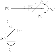
Figure 12: Alice and Bob apply a local unitary operation on her/his mode $a$ and $b$.

The fact that this local unitary operation exists tells us that there ought to be a nonlocal measurement which acknowledges this fact. Therefore the same amount of nonlocality should be obtained for the $N$-photon state as for the one-photon entangled state. The fact that some of the Bell-tests do not show this result means that these Bell-tests are not optimal. However the Bell-tests of the inequalities in Eqs. (22,23,25) seem to be optimal for the N00N state since their outcome shows a constant violation for any $N$. We point out that these Bell-type inequalities have two more joint probabilities than the CH and CHSH Bell inequalities. The class of inequalities with six joint probabilities seem to be more sensitive to the nonlocality in N00N states. From our results we also infer, that for some applications, types of Bell inequalities other than the Clauser-Horne and the Clauser-Horne-Shimony-Holt should be considered. It is, experimentally, not more difficult to test these Bell inequalities; since one only needs to measure the correlation functions for a few more parameter settings. The experimental setup does not need to be changed.

V Conclusion

We presented several Bell-tests for N00N states. In section II a simple on-off detection scheme together with the CH Bell inequality shows a violation for any $N$ although the violation decreases as $N$ increases. In section III we consider a correlated parity measurement together with the CHSH Bell inequality. A violation is found only for $N=1$. In section IV we consider the simple on-off detection scheme but test Bell-type inequalities with six joint probabilities. We then attain a violation that stays constant for any $N$ and we show by a simple argument with local unitary operations that this is to be expected for an optimal Bell-test with N00N states. If we use the violation of a Bell-type inequality as a measure of nonlocality then N00N states contain the same amount of nonlocality for any $N$. Despite this fact, using N00N states with large $N$ is advantageous for applications like quantum imaging, metrology, and sensing, although the improvement in the performance of these applications does not seem to be necessarily related to the nonlocal properties of N00N states.

Finally we point out that it might be advantageous in many experiments to also test the Bell-type inequalities in section IV, in addition to the CH or CHSH Bell inequalities. One gains more insight into the nonlocal properties of the states under investigation, as shown by our example.

- (1) B. C. Sanders, Phys. Rev. A. 40, 2417 (1989); A. N. Boto, et al., Phys. Rev. Lett. 85, 2733 (2000).
- (2) H. Lee, P. Kok, and J. P. Dowling, J. Mod. Opt. 49, 2325 (2002).
- (3) A. Migdall, Physics Today 52, 95 (1999).
- (4) K. T. Kapale, L. D. Didomenico, H. Lee, P. Kok, and J. P. Dowling, Concepts of Physics, Vol II, 225 (2005).
- (5) M. Genovese, Phys. Rep. 413, 319 (2005).
- (6) R. F. Werner, Phys. Rev. A 40, 4277 (1989).
- (7) M. D. Reid and D. F. Walls, Phys. Rev. A 34, 1260 (1986); S. M. Tan, D. F. Walls, and M. J. Collett, Phys. Rev. Lett. 66, 252 (1991); L. Hardy, Phys. Rev. Lett. 73, 2279 (1994); D. M. Greenberger, M. A. Horne, and A. Zeilinger, Phys. Rev. Lett. 75, 2064 (1995); L. Hardy, Phys. Rev. Lett. 75, 2065 (1995); S. J. van Enk, Phys. Rev. A 72, 064306 (2005).
- (8) N. Gisin and A. Peres, Phys. Lett. A 162, 15 (1992).
- (9) S. Popescu and D. Rohrlich, Phys. Lett. A 166, 293 (1992).
- (10) S. A. Babichev, J. Appel, and A. I. Lvovsky, Phys. Rev. Lett. 92, 193601 (2004); B. Hessmo, P. Usachev, H. Heydari, and G. Björk, Phys. Rev. Lett. 92, 180401 (2004).
- (11) M. D’Angelo, A. Zavatta, V. Parigi, and M. Bellini, Phys. Rev. A 74, 052114 (2006).
- (12) K. Banaszek and K. Wódkiewicz, Phys. Rev. Lett. 82, 2009 (1999).
- (13) S. D. Bartlett, A. C. Doherty, R. W. Spekkens, and H. M. Wiseman, Phys. Rev. A 73, 022311 (2006).
- (14) S. J. van Enk, Phys. Rev. A 72, 064306 (2005).
- (15) S. J. van Enk, Phys. Rev. A 74, 026302 (2006).
- (16) H. M. Wiseman and G. J. Milburn, Phys. Rev. Lett. 70, 548 (1993).
- (17) K. Banaszek and K. Wódkiewicz, Phys. Rev. Lett 76, 4344 (1996).
- (18) S. Wallentowitz and W. Vogel, Phys. Rev. A 53, 4528 (1996).
- (19) J.F. Clauser and M. A. Horne, Phys, Rev. D 10, 526 (1974).
- (20) A. Royer, Phys. Rev. A 15, 449 (1977).
- (21) H. Moya-Cessa and P. L. Knight, Phys. Rev. A 48, 2479 (1993).
- (22) M. Abramowitz and I. A. Stegun, Handbook of Mathematical Functions with formulas, graphs, and mathematical tables. (Wiley, New York 1972).
- (23) J. F. Clauser, M. A. Horne, A. Shimony, and R. A. Holt, Phys. Rev. Lett. 23, 880 (1969).
- (24) I. Pitowsky, Quantum Probability–Quantum Logic, Lecture Notes in Physics 321, Springer, Berlin, New York, (1989).
- (25) S. Janssens, B. De Baets, and H. De Meyer, Fuzzy Sets and Systems 148, 263-278 (2004).