Security of quantum key distribution protocols using two-way classical communication or weak coherent pulses

Abstract

We apply the techniques introduced in [Kraus et. al., Phys. Rev. Lett., 95, 080501, 2005] to prove security of quantum key distribution (QKD) schemes using two-way classical post-processing as well as QKD schemes based on weak coherent pulses instead of single-photon pulses. As a result, we obtain improved bounds on the secret-key rate of these schemes.

I Introduction

A fundamental problem in cryptography is to enable two distant parties, traditionally called Alice and Bob, to communicate in absolute privacy, even in presence of an eavesdropper, Eve. It is a well known fact that a secret key, i.e., a randomly chosen bit string held by both Alice and Bob, but unknown to Eve, is sufficient to perform this task (one-time pad encryption). Thus, the problem of secret communication reduces to the problem of distributing a secret key.

Classical key distribution protocols are typically based on unproven computational assumptions, e.g., that the task of decomposing a large number into its prime factors is intractable. In contrast to that, the security of quantum key distribution (QKD) protocols merely relies on the laws of physics, or, more specifically, quantum mechanics. This ultimate security is certainly one of the main reasons why so much theoretical and experimental effort is undertaken towards the implementation of secure QKD protocols GiRi02 ; IdqMQ .

Typically , in the first step of a QKD protocol, Alice chooses a random bit string and encodes each bit into the state of a quantum system, which she then sends to Bob (using a quantum channel). Bob applies a certain measurement on the received quantum system to decode the bit value. In a second step, called sifting, Alice and Bob publicly exchange some information about the encoding and decoding of each of the bits which allows them to discard bit pairs which are not (or only weakly) correlated.

After this sifting process, Alice and Bob hold a pair of classical correlated bitstrings, in the following called raw key pair. Alice and Bob can determine the quality of the raw key pair by comparing the values of some randomly chosen bit pairs (using an authenticated classical communication channel). This so-called parameter estimation gives an estimate for the quantum bit error rate (QBER), i.e., the ratio of positions for which the values of the bits held by Alice and Bob do not coincide. A fundamental principle of QKD is that this error rate also imposes a bound on the amount of information an adversary can have on the raw key: The smaller the QBER, the more secret key bits can be extracted from the raw key. If the QBER is above a certain threshold, then no secret key can be generated at all, and Alice and Bob have to abort the protocol .

The purpose of the remaining part of the protocol, called classical post-processing, is to transform the raw key pair into a pair of identical and secret keys. In this article, we consider classical post-processing which consists of the following three subprotocols: (i) local randomization (also called pre-processing), where Alice randomly flips each of her bits with some given probability $q$, (ii) error correction, where Alice and Bob equalize their strings, and (iii) privacy amplification, where Alice and Bob apply some compression function to their bitstring with the aim to reduce Eve’s information on the outcome. Steps (i)–(iii) described above only require (classical) one-way communication from Alice to Bob. However, in practical implementations, the error correction is sometimes done with two-way protocols (e.g., the cascade protocol BrSa94 ).

In KrRe05 ; ReKr05 , an information-theoretic technique to analyze QKD protocols of the type described above has been presented. In contrast to most previously known methods (e.g., ShPr00 ), the technique does not require a transformation of the key distillation protocol into an entanglement purification scheme, which makes it very general. It has been applied to prove the security of various schemes such as the BB84, the six-state, the B92, and the SARG protocol BB84 ; BeGi99 ; Be92 ; ScAc04 (see KrRe05 ; ReKr05 for an analysis of the first three protocols and BrGi05 for an analysis of the latter). In particular, it has been shown that the local randomization, i.e., step (i) described above, increases the bounds on the maximum tolerated QBER by roughly 10–15 %.

In this paper, we extend the technique of KrRe05 ; ReKr05 (Section II) and apply it to two classes of QKD protocols which have not been covered in KrRe05 ; ReKr05 . The first (Section III) is the class of so-called two-way protocols. These use an additional subprotocol, called advantage distillation, which is invoked between the parameter estimation and the classical post-processing step described above. In contrast to the classical post-processing considered in KrRe05 ; ReKr05 , advantage distillation uses two-way communication between Alice and Bob. Second, we study protocols which use weak coherent pulses instead of single-photon pulses (Section IV). For both scenarios, we show that local randomization increases the secret-key rates.

II Information-theoretic analysis of QKD schemes

In this section we first review the results presented in  KrRe05 ; ReKr05 and then show then show how they can be generalized. Throughout this paper we use subscripts to indicate the subsystems on which a state is defined. Alice and Bob’s quantum systems are labelled by $A$ and $B$, respectively. Similarly, the classical values obtained by measuring their quantum systems are denoted by $X$ and $Y$, respectively. Typically, we write $\rho_{AB}$, or $\rho_{n}$, to denote the state of all the qubits held by Alice and Bob, whereas $\sigma_{AB}$ is a two-qubit state. We will often consider two-qubit Bell-diagonal states, i.e., states that are diagonal in the Bell basis, $|\Phi_{ij}\rangle=(|0,0+i\rangle+(-1)^{j}|1,1+i\rangle)/\sqrt{2}$. $P_{|\Phi\rangle}$ denotes the projector onto the state ${|\Phi\rangle}$. Furthermore, we denote by $h(x)=-x\log_{2}(x)-(1-x)\log_{2}(1-x)$ the binary entropy function.

II.1 Review of the technique

The information-theoretic technique proposed in KrRe05 ; ReKr05 directly applies to a general class of quantum key distribution protocols using one-way classical communication. However, it is required that the protocol can be represented as a so-called entanglement-based scheme, as described below.

Generally, a QKD protocol uses a set of so-called encoding bases. We consider the special case where each basis $j$ is defined by two states $|\phi_{j}^{0}\rangle$ and $|\phi_{j}^{1}\rangle$, which are used to encode the bit values $0$ and $1$, respectively. In a prepare-and-measure scheme, Alice repeatedly chooses at random a bit $i$ and a basis $j$, prepares the state $|\phi_{j}^{i}\rangle$, and sends the state to Bob. Bob then measures the state in a randomly chosen basis $k$. This measuring process can be seen as some filtering operation $B_{k}=|0\rangle\langle\phi_{1,k}^{\perp}|+|1\rangle\langle\phi_{0,k}^{\perp}|$, where $|\phi_{i,k}^{\perp}\rangle$ is some state orthogonal to $|\phi_{k}^{i}\rangle$, followed by a measurement in the computational basis.

In an entanglement-based view, the above can equivalently be described as follows: Alice prepares the two-qubit states $A_{j}|\Phi_{00}\rangle$, where $|\Phi_{00}\rangle$ denotes the Bell state $1/\sqrt{2}(|0,0\rangle+|1,1\rangle)$ and $A_{j}$ is an encoding operator (for details see KrRe05 ) such that $\langle i|A_{j}|\Phi_{00}\rangle=|\phi_{j}^{i}\rangle$. She then sends the second qubit to Bob and prepares Bob’s system at a distance by measuring her system in the computational basis. Bob’s measurement is described in the same way as in the prepare-and-measure scheme.

Note that, in an experimental realization of a QKD protocol, one might prefer to implement a prepare-and-measure scheme. However, when analyzing the security of a protocol, it is usually more convenient to consider its entanglement-based version.

As an illustration, consider the BB84 protocol, which uses the $z$-basis and the $x$-basis are used for the encoding. Using the above notation, we have $|\phi_{0}^{i}\rangle=|i_{z}\rangle$ and $|\phi_{1}^{i}\rangle=|i_{x}\rangle$, for $i=0,1$. Hence, the operators applied by Alice are $A_{0}=\mbox{$1{\bf l}$}$ and $A_{1}=H$, where $H$ denotes the Hadamard transformation. Because the bases are orthonormal, the same operators describe Bob’s measurement as well.

For the following, we assume that Alice and Bob apply a randomly chosen permutation to rearrange the order of their qubit pairs, in the following denoted by $\mathcal{P}_{S}$, and, additionally, apply to each of the qubit pairs at random either the identity or the operation $\sigma_{x}\otimes\sigma_{x}$. (Note that the symmetrization operations commute with the measurement and can therefore be applied to the classical bit strings). Then, as shown in KrRe05 , the state $\rho_{AB}$ describing the $N$ qubit pairs shared by Alice and Bob can generally (after the most general attack by Eve, a so-called coherent attack) be considered to be of a simple form, namely

$$\rho_{AB}=\sum_{n_{1},\ldots,n_{4}}\lambda_{n_{1},n_{2},n_{3},n_{4}}\mathcal{P}_{S}(P_{|\Phi_{00}\rangle}^{\otimes n_{1}}\otimes P_{|\Phi_{01}\rangle}^{\otimes n_{2}}\otimes P_{|\Phi_{10}\rangle}^{\otimes n_{3}}\otimes P_{|\Phi_{11}\rangle}^{\otimes n_{4}})\ .$$ (1)

The sum runs over all nonnegative $n_{1},\ldots,n_{4}$ such that $n_{1}+n_{2}+n_{3}+n_{4}=N$. The set of possible values of the coefficients $\lambda_{n_{1},n_{2},n_{3},n_{4}}$ depends on the specific protocol and the parameters estimated by Alice and Bob (e.g., the QBER of the raw key). Furthermore, one can assume without loss of generality that Eve has a purification of this state, i.e., the situation is fully described by a pure state $|\Psi\rangle_{ABE}$ such that $\rho_{AB}=\mathrm{tr}_{E}(P_{|\Psi\rangle_{ABE}})$. (However, as we shall see, dropping this assumption might lead to better estimates of the key rate.) After this distribution of quantum information Alice and Bob measure their systems. Thus they are left with classical bit-strings.

Consider now any situation where Alice and Bob have a classical pair of raw keys $X^{n}$ and $Y^{n}$ consisting of $n$ bits whereas Eve controls a quantum system $E$. The secret-key rate, i.e., the rate at which secret key bits can be generated per bit of the raw key, for any one-way protocol (with communication from Alice to Bob), is given by

$$r=\lim_{\varepsilon\to 0}\lim_{n\rightarrow\infty}\frac{1}{n}\sup_{U^{n}\leftarrow X^{n}}S_{2}^{\varepsilon}(U^{n}E^{n})-S_{0}^{\varepsilon}(E^{n})-H_{0}^{\varepsilon}(U^{n}|Y^{n})\ .$$ (2)

Here, $S_{\alpha}^{\varepsilon},H_{\alpha}^{\varepsilon}$ denote the smooth Rényi entropies (also called min-entropy if $\alpha=\infty$ and max-entropy if $\alpha=0$) ThesisRe . Moreover, the supremum runs over all classical values $U^{n}$ that can be computed from (the classical value) $X^{n}$.

For a QKD protocol as described above (where the distributed state is of the form of Eq. (1)), formula (2) can be lower bounded by an expression which only involves two-qubit systems. More precisely KrRe05 ,

$$r\geq\sup_{\begin{subarray}{c}U\leftarrow X\end{subarray}}\,\inf_{\sigma_{AB}\in\Gamma_{Q}}S(U|E)-H(U|Y)\ ,$$ (3)

where $\Gamma_{Q}$ is the set of all two-qubit states $\sigma_{AB}$ (after the filtering operation) which can result from a collective attack  and which are compatible with the parameters estimated by Alice and Bob (in particular, the QBER). Here, $S$ and $H$ denote the von Neumann entropy and its classical counterpart, the Shannon entropy, respectively. Moreover, $X$ and $Y$ denote the classical outcomes of measurements of $\sigma_{AB}$ (on $A$ and $B$, respectively) in the computational basis, and $E$ is any system that purifies $\sigma_{AB}$. Similarly to the above formula, the supremum runs over all mappings from $X$ to $U$ .

II.2 Local randomization

The local randomization step described above has first been considered in KrRe05 ; ReKr05 and later been improved in  SmReSm06 . In RenSmis06 , the local randomization is nicely explained in the context of entanglement purification.

To get an intuition why the local randomization can help to increase the secret-key rate, it is useful to describe the process as a quantum operation (as in RenSmis06 ). Let $\sigma_{AB}$ be the state of a qubit pair held by Alice and Bob and let $|\Psi\rangle_{ABE}$ be a purification of $\sigma_{AB}$. The state after Alice randomly flips her bit value $A$ with probability $q$, can be described by $|\Psi\rangle_{AA^{\prime}BE}=\sqrt{1-q}|\Psi\rangle_{ABE}|0\rangle_{A^{\prime}}+\sqrt{q}\sigma_{x}^{A}|\Psi\rangle_{ABE}|1\rangle_{A^{\prime}}$, where $A^{\prime}$ is an auxiliary system on Alice’s side. The measurement of system $A$ gives the raw key. Note that $|\Psi\rangle_{AA^{\prime}BE}$ results from the application of a controlled-not operation on system $AA^{\prime}$, where system $A^{\prime}$ is prepared in the state $\sqrt{1-q}|0\rangle_{A^{\prime}}+\sqrt{q}|1\rangle_{A^{\prime}}$. The randomization of Alice thus entangles her system to some auxiliary system (which is not under Eve’s control). This, in turn, reduces the entanglement between Alice’s relevant system ($A$) and Eve’s systems (monogamy of entanglement), as Eve does not have a purification of the state on the systems $A$ and $B$, since now she only has the purification of the state $\rho_{AA^{\prime}B}$. Note that Bob’s information on $A$ is also reduces by the randomization process, but—for certain values of the parameter $q$—he is less penalized than Eve. From this point of view, it can be easily understood that the local randomization can help to increase the secret-key rate.

II.3 Comparison to known bounds

For protocols based on qubit pairs, where the raw key pair is obtained by orthogonal measurements of Alice and Bob on some Bell-diagonal state $\sigma_{AB}=\sum_{i,j}\lambda_{ij}P_{\Phi_{ij}}$ (e.g., the BB84 or the six-state protocol), it follows from (3) that the secret-key rate $r$ (even without the local randomization) is bounded by

$$r\geq 1-S(\sigma_{AB})\geq 1-h(e_{b})-h(e_{p})\ .$$

Here, $e_{b}=\lambda_{10}+\lambda_{11}$ is the QBER and $e_{p}=\lambda_{01}+\lambda_{11}$ the phase error rate, i.e., the probability that Alice and Bob get different bits when measuring in the $z$ and the $x$-basis, respectively. Because the QBER and the phase error rate are not changed by applying at random $\sigma_{x}$ or $\sigma_{z}$, which make any state Bell diagonal, the bound $1-h(e_{b})-h(e_{p})$ holds for arbitrary states $\sigma_{AB}$. Note that the above bound implies any of the lower bounds on the one-way secret-key rate derived in previous works ShPr00 ; Lo01 .

II.4 Generalization of the lower bound

Because we assume above that Eve controls a system that purifies the state $\rho_{AB}$ held by Alice and Bob, the bound (3) is fully determined by $\rho_{AB}$. However, this assumption on Eve might overestimate her possibilities, in which case the bound is not optimal. In the following we drop this assumption to derive better lower bounds on the secret-key rate.

Suppose that the state distributed in an entanglement-based scheme is of the form $\mathcal{P}_{S}((\mathcal{D}_{AB}\otimes\mbox{$1{\bf l}$})^{\otimes n}(\rho^{0}_{ABE}))$, where $\mathcal{P}_{S}$ again denotes the map that randomly permutes the order of the qubit pairs, $\mathcal{D}_{AB}$ is some completely positive map on two-qubit states, and $\rho^{0}_{ABE}$ is some tripartite state. Then, it is an immediate consequence of Lemma A.4 in ReKr05 that the bound (3) on the secret-key rate can be generalized to

$$r\geq\sup_{\begin{subarray}{c}U\leftarrow X\end{subarray}}\,\inf_{\tilde{\sigma}_{ABE}\in\tilde{\Gamma}_{Q}}S(U|E)-H(U|Y)\ .$$ (4)

Here, the infimum ranges over the set $\tilde{\Gamma}_{Q}$ of all states $\tilde{\sigma}_{ABE}$ which can result from a collective attack and are compatible with the parameters estimated by Alice and Bob (e.g., the QBER).

We refer to Appendix C for an application of this result to improve the analysis of the one-way SARG protocol for single-photon pulses.

Consider now the general situation where the state describing Alice, Bob, and Eve’s system is the reduced density operator of a state $|\Psi\rangle_{ABER}=\sum_{n}\alpha_{n}|\Psi_{n}\rangle_{ABE}|n\rangle_{R}$, where $\{|n\rangle\}$ forms an orthonormal basis of the Hilbert space of an auxiliary system $R$, i.e., none of the three parties has the auxiliary system at their disposal. Starting from (4) and using the concavity of the entropy, we find that the secret-key rate is bounded by

$$r\geq\sup_{U\leftarrow X}\inf_{\tilde{\sigma}_{ABE}\in\tilde{\Gamma}_{Q}}\Bigl{(}\sum_{n=0}^{\infty}|\alpha_{n}|^{2}S(U|E,n)\Bigr{)}-H(U|Y),$$ (5)

where $S(U|E,n)=S(UE|n)-S(E|n)$, is the entropy of $U$ conditioned on $E$ and the event that the measurement of the auxiliary system $R$ in the basis $\{|n\rangle\}$ yields $n$.

One might also improve the bound using the following observation which has also been used to derive the bound given in Eq. (3). Let us consider the situation where some auxiliary system is at Alice’ and/or Bob’s disposal, but not at Eve’s (this could be for instance some additional qubits). Suppose that the state shared by $ABE$ and some auxiliary system $R$ (which is not under Eve’s control) is given by $|\Psi\rangle_{ABER}=\sum_{n}\alpha_{n}|\Psi_{n}\rangle_{ABE}|n\rangle_{R}$, where $\{|n\rangle\}$ is an orthonormal basis of ${\cal H}_{R}$, the Hilbert space corresponding to system $R$. The state $|\tilde{\Psi}\rangle_{ABER}=\sum_{n}\alpha_{n}U^{AB}_{n}|\Psi_{n}\rangle_{ABE}|n\rangle_{R}$, with $U^{AB}_{n}$ unitary operators diagonal in the $z$-basis leads to the same measurement outcome for any measurement by Alice and Bob in the computational basis as $|\Psi\rangle_{ABER}$, that is $|k,l\rangle_{AB}\langle k,l|\rho_{ABE}|k,l\rangle_{AB}\langle k,l|=|k,l\rangle_{AB}\langle k,l|\tilde{\rho}_{ABE}|k,l\rangle_{AB}\langle k,l|$, where $\rho_{ABE}=\mathrm{tr}_{R}(P_{|\Psi\rangle_{ABER}})$ and $\tilde{\rho}_{ABE}=\mathrm{tr}_{R}(P_{|\tilde{\Psi}\rangle_{ABER}})$. Assuming that Eve has a purification of the state $\tilde{\rho}_{AB}$ can only provide her with more power compared to the situation where she has a purification of the state $\rho_{ABR}$, since this is equivalent to giving her the system $R$, which she could simply measure, leading to the same result as before (for details see also KrRe05 ). Thus, we can consider the situation where Alice and Bob share the state $\tilde{\rho}_{AB}$ and Eve has a purification of it. This can only increase Eve’s power. We will use this observation in Appendix B, in order to determine a good lower bound on the secret-key rate for a QKD protocol using the so-called XOR process.

III QKD protocols with two-way post-processing

In the following, we will consider QKD protocols where, before the post-processing of the raw key as described above, Alice and Bob additionally invoke a so-called advantage-distillation subprotocol, which requires two-way communication between Alice and Bob. The notion of advantage distillation has first been investigated in the context of classical key agreement Maurer93 and later been generalized to QKD GoLo03 ; Ch02 .

The advantage distillation protocol we consider here has the following form: Alice publicly announces to Bob the position of a block of $m$ bits which have all the same value (of course, she does not tell him which value). Then Bob tells Alice whether for the given position, his corresponding bits are all identical as well. If this is the case, they both continue using the first bit of the block as a new raw-key bit, otherwise they discard the whole block. We emphasize here that our analysis below works for any fixed value of the block size $m$ (not only asymptotically for large $m$). This is important for realistic protocols, where $m$ is usually small (e.g., $m=3$).

To simplify the study of such protocols, we first show that it suffices to analyze the action of the advantage distillation process on two-qubit Bell-diagonal states. More precisely, Lemma 1 below implies that the state $\bar{\rho}_{\bar{n}}$ obtained by applying a block-wise operation $\mathcal{E}$ (for blocks of size $m$) to a symmetric state $\rho_{n}$ (see Eq. (1)) has virtually the same statistics as if $\mathcal{E}$ was applied to a state $\sigma^{\otimes m}$.

Lemma 1.

Let $\rho_{n}$ be a state on $n$ particle pairs of the form

$$\rho_{n}=\mathcal{P}_{S}(P_{|\Phi_{00}\rangle}^{\otimes n_{1}}\otimes P_{|\Phi_{01}\rangle}^{\otimes n_{2}}\otimes P_{|\Phi_{10}\rangle}^{\otimes n_{3}}\otimes P_{|\Phi_{11}\rangle}^{\otimes n_{4}})$$

and let $\sigma$ be a two-qubit Bell-diagonal state with eigenvalues $\frac{n_{1}}{n},\ldots,\frac{n_{4}}{n}$. Moreover, let $\mathcal{E}$ be an operation which maps Bell states of blocks of $m$ particle pairs to Bell states of one single particle pair. Finally, let

$$\bar{\rho}_{\bar{n}}=\sum_{\bar{n}_{1},\ldots,\bar{n}_{4}}\bar{\mu}_{\bar{n}_{1},\bar{n}_{2},\bar{n}_{3},\bar{n}_{4}}{\cal P}_{S}(P_{|\Phi_{00}\rangle}^{\otimes\bar{n}_{1}}\otimes P_{|\Phi_{01}\rangle}^{\otimes\bar{n}_{2}}\otimes P_{|\Phi_{10}\rangle}^{\otimes\bar{n}_{3}}\otimes P_{|\Phi_{11}\rangle}^{\otimes\bar{n}_{4}})$$

be the state describing $\bar{n}=\frac{n}{m}$ particle pairs defined by $\bar{\rho}_{\bar{n}}:=\mathcal{E}^{\otimes\bar{n}}(\rho_{n})$ and let $\bar{\lambda}_{1},\ldots,\bar{\lambda}_{4}$ be the eigenvalues of $\bar{\sigma}:=\mathcal{E}(\sigma^{\otimes m})$. Then, for any $\varepsilon\geq 0$,

$$\sum_{(\bar{n}_{1},\ldots,\bar{n}_{4})\in\mathcal{B}^{\varepsilon}(\bar{\lambda}_{1},\ldots,\bar{\lambda}_{4})}\bar{\mu}_{\bar{n}_{1},\bar{n}_{2},\bar{n}_{3},\bar{n}_{4}}\geq 1-2^{-\Theta(\bar{n}\varepsilon^{2})+O(\log n)},$$

where $\mathcal{B}^{\varepsilon}(\bar{\lambda}_{1},\ldots,\bar{\lambda}_{4})$ denotes the set of all tuples $(\bar{n}_{1},\ldots,\bar{n}_{4})$ such that $(\frac{\bar{n}_{1}}{n},\ldots,\frac{\bar{n}_{4}}{n})$ is $\varepsilon$-close to $(\bar{\lambda}_{1},\ldots,\bar{\lambda}_{4})$ and $\Theta(\bar{n}\varepsilon^{2})$ is asymptotically the same as $\bar{n}\varepsilon^{2}$, up to a constant factor.

The lemma is a direct consequence of the exponential quantum de Finetti Theorem ThesisRe . It states that, for any $n$-partite quantum state $\rho_{n}$ which is invariant under permutations of the subsystems, any part $\rho_{m}=\mathrm{tr}_{n-m}(\rho_{n})$ consisting of $m$ subsystems is exponentially (in $n-m$) close to a convex combination of states that virtually are of the form $\sigma^{\otimes m}$. For completeness, we give a direct proof of Lemma 1 (without referring to de Finetti’s theorem) in Appendix A.

In order to analyze protocols with advantage distillation using Lemma 1, we use the following quantum mechanical description of the advantage distillation subprotocol: Alice and Bob both apply the operation $X^{m}_{ad}=|0\rangle\langle 0,\ldots,0|+|1\rangle\langle 1,\ldots,1|$ on $m$ qubits. It is straightforward to check that

$$(X^{2}_{ad})^{\otimes 2}(|\Phi_{i,j}\rangle|\Phi_{k,l}\rangle)=\frac{1}{\sqrt{2}}\delta_{i,k}|\Phi_{i,j+l}\rangle,$$ (6)

where the sum $j+l$ of indices is understood to be modulo $2$. Hence, applying advantage distillation to $m$ identical Bell-diagonal qubit-pairs with eigenvalues $\lambda$  leads to a Bell-diagonal state with eigenvalues $\lambda^{\prime}$ given by

$$\lambda_{i,j}^{\prime} =\frac{1}{T}\big{[}(\lambda_{i,0}+\lambda_{i,1})^{m}+(-1)^{j}(\lambda_{i,0}-\lambda_{i,1})^{m}\big{]}\,$$ (7)

where $T=2[(1-Q)^{m}+Q^{m}]$ and where $Q=\lambda_{10}+\lambda_{11}$ is the QBER before the advantage distillation. The QBER $Q^{\prime}$ after the advantage distillation is thus given by $Q^{\prime}=\lambda_{10}^{\prime}+\lambda_{11}^{\prime}=\frac{Q^{m}}{(1-Q)^{m}+Q^{m}}$ and $(1-Q)^{m}+Q^{m}$ is the probability that the advantage distillation is successful (i.e., Alice and Bob end up with a new raw key bit). If Alice and Bob apply, after the advantage distillation the one-way classical post-processing described above, the lower bound on the secret-key rate is given by Eq. (3), where the eigenvalues of $\sigma_{AB}$ are given by the $\lambda$‘s in (7) . For instance for the six-state protocol one obtains a positive key rate for any $QBER<0.276$ (for $m\longrightarrow\infty$). Note that for the six-state protocol it has been shown that the tolerable QBER cannot be larger than $0.276$, if the first step in the post-processing is advantage distillation AcMa . As mentioned before, the bound on the secret-key rate is not only valid, for $m\longrightarrow\infty$, but for any value of the block size on which advantage distillation is applied.

In Ch02 , Chau considered the secret-key rate obtained when applying the above described advantage distillation followed by the XOR transformation, where Alice and Bob locally compute new raw key bits by taking the XOR of a block of given bits. (For the sake of completeness we demonstrate in Appendix B, how the XOR protocol can be included in our analysis.) Both procedures were analyzed in the asymptotic limit for infinitely large block sizes. The result found there is that the six-state protocol tolerates a QBER of up to $0.276$. Surprisingly, the same threshold for the QBER can be obtained, as shown above, by a simpler protocol where the XOR transformation is replaced by a local randomization on single bits on Alice’s side. Moreover, the rate of this modified protocol is much larger than that of Chau’s protocol, as local randomization consumes less bits than the XOR transformation. Note that, as shown recently by Bae and Acin Acin06 , if one omits the local randomization completely, the protocol still tolerates a QBER of up to $0.276$, but the secret-key rate for large values of the QBER might be smaller.

IV Protocols using weak coherent pulses

IV.1 Preliminaries

We now consider protocols where Alice does not send single photons to Bob, but uses weak coherent pulses instead. This scenario is practically motivated by the fact that, with current technologies, it is difficult to create single-photons pulses. In fact, many of today’s implementations of QKD rely on weak coherent pulses.

We start with a description of a prepare-and-measure scheme and then translate it to an equivalent entanglement based scheme, for which we will prove security.

In the prepare-and-measure scheme, Alice encodes the bit values into phase randomized coherent states . More precisely, she randomly chooses a basis $j$ and encodes the bit value $k$ into the state $\rho_{j}^{k}=\sum_{n\geq 0}p_{n}|\phi_{j}^{k}\rangle\langle\phi_{j}^{k}|^{\otimes n}$, where $|\phi_{j}^{k}\rangle\langle\phi_{j}^{k}|^{\otimes 0}$, denotes the vacuum for any value of $j$ and $k$ and $p_{n}=e^{-\mu}\mu^{n}/n!$, with $\mu$ the mean photon number (for a Poissonian source ).

The description of Bob’s measurement depends on the experimental setup. We focus on the situation where Bob’s detectors do not distinguish between the cases where they receive one or more than one photons, since with current technology, it is difficult to count the number of photons. The POVM describing the photon detector is thus given by the operators $\{D_{0}^{\dagger}D_{0},D_{1}^{\dagger}D_{1}\}$, with $D_{0}=\sum_{n\geq 0}\sqrt{p_{n.d.}(n)}P_{|n\rangle}$ and $D_{1}=\sum_{n\geq 0}\sqrt{1-p_{n.d.}(n)}P_{|n\rangle}$, where $p_{n.d.}(n)$ is the probability of not detecting any photon in case $n$ photons arrived at the detector. This probability is given by $p_{n.d.}(n)=(1-p_{d})(1-\eta)^{n}$, where $p_{d}$ is the probability of a dark count, and $\eta$ is the detection efficiency, i. e. overall transmission factor. The POVM element $D_{0}$ corresponds to the case where no photon is detected, whereas $D_{1}$ corresponds to the detection of one or more photons. In the prepare-and-measure scheme Bob would randomly choose a basis $j$ and measure the arriving photons in that basis.

In the following, we consider the so-called untrusted-device scenario, where it is assumed that Eve exchanges Bob’s detectors with perfect ones (having perfect efficiency and no dark counts) and introduces all errors herself . Clearly, security under this assumption implies security in a situation where Eve might not be able to corrupt Bob’s detectors. Additionally, we assume that Bob’s detector is constructed in such a way that, whenever a pulse consisting of more than one photon arrives, then the detector output corresponds to the measurement of one of the photons in the pulse chosen at random .

In the described scenario, we can without loss of generality assume that Eve only sends single photons to Bob. This follows directly from the fact that the situation obtained by sending a multi-photon pulse is the same as if Eve randomly selected one photon from the pulse and sent this single photon to Bob. Bob’s measurement can therefore simply be described by the operators $B_{j}=|0\rangle\langle\phi_{1,j}^{\perp}|+|1\rangle\langle\phi_{0,j}^{\perp}|$ as defined previously.

Alice and Bob can estimate the following parameters related to their raw key: (i) the total sifting rate $R_{\mu}:=\sum_{n}R_{n}$, for $R_{n}:=p_{n}Y_{n}$ where $Y_{n}$ is the probability for Bob to find a conclusive result in case Alice sent $n$ photons; (ii) the average QBER $Q_{\mu}=\sum_{n}\frac{R_{n}}{R_{\mu}}Q_{n}$, where $Q_{n}$ denotes the QBER for the pairs where Alice sent an $n$-photon pulse. These two parameters will determine the amount of key that can be extracted from the particular raw key.

We use similar techniques as in KrRe05 ; ReKr05 to describe the same protocol in the entanglement-based scheme. The states prepared by Alice are

$$|\Psi_{j}\rangle_{ABR_{1}}=\sum_{n\geq 0}\sqrt{p_{n}}|\Psi_{j}^{n}\rangle_{AB}|n\rangle_{R_{1}},$$ (8)

where $|\Psi_{j}^{n}\rangle_{AB}=1/\sqrt{2}(|0\rangle_{A}|\phi_{j}^{0}\rangle_{B}^{\otimes n}+|1\rangle_{A}|\phi_{j}^{1}\rangle_{B}^{\otimes n})$. Here, we have introduced an auxiliary system $R_{1}$ containing the photon number (which is neither controlled by Alice nor Bob). If Alice measures her qubit in the computational basis and receives outcome $k$, the state Bob is left with in the noiseless case (without interaction of Eve) is $\rho_{B}=2\mathrm{tr}_{R_{1}}(P_{\langle k|\Psi_{j}\rangle_{ABR_{1}}})=\sum_{n\geq 0}p_{n}P_{|\phi_{j}^{k}\rangle^{\otimes n}}$, which corresponds to the coherent state (with randomized phase) sent by Alice in the prepare-and measure scheme . The operation on Bob’s side is given by the operators $B_{j}$, as described above.

The state describing the situation after Bob’s operation is given by

$$|\chi\rangle_{ABER_{1}R_{2}}=\sum_{j}B_{j}U_{EB}(|\Psi_{j}\rangle_{ABR_{1}})|j\rangle_{R_{2}}\ ,$$

where $j$ corresponds to the basis chosen by Alice and $U_{EB}$ is a unitary describing the attack of Eve. Note that this state is not necessarily normalized, but its weight $\mathrm{tr}(|\chi\rangle\langle\chi|)$ corresponds to the sifting rate.

Restricted to Alice and Bob’s systems, $|\chi\rangle_{ABER_{1}R_{2}}$ is a two-qubit state. We can thus apply the techniques presented in Section II to analyze the security of the protocol. More precisely, we need to evaluate the r.h.s. of (5) to get a lower bound on the secret-key rate. First we do not take the local randomization into account, i.e., we choose $U=X$. The case including local randomization will be treated in the next subsection. We thus obtain, for the key rate

$$r\geq\inf_{\sigma\in\Gamma_{R_{\mu},Q_{\mu}}}\sum_{n=0}^{\infty}R_{n}S(X|E,n)-R_{\mu}S(X|Y).$$ (9)

The set $\Gamma_{R_{\mu},Q_{\mu}}$ contains all states which can result from a collective attack by Eve and are compatible with the average sifting rate $R_{\mu}$ and the QBER $Q_{\mu}$, as estimated by Alice and Bob.

Because the (conditional) entropy of a classical variable cannot be negative, the r.h.s. of (9) can be lower bounded by restricting to any of the terms in the sum over $n$. Note that, in (9), the average over $n$ is only taken over the term for the entropy conditioned on Eve’s system, but not on the term for the entropy conditioned on Bob’s system. This is because Eve might be able to measure the photon number, whereas this is not the case for Bob.

IV.2 Protocols with local randomization

So far we did not consider the possibility for Alice to apply some local randomization on her classical bits. The randomization can easily be included in the analysis: if the randomization is acting on single bits, $U\leftarrow X$ (bit flip with probability $q$), (9) simply writes

$$r\geq\inf_{\sigma\in\Gamma_{R_{\mu},Q_{\mu}}}\sum_{n=0}^{\infty}R_{n}S(U|E,n)-R_{\mu}S(U|Y).$$ (10)

Bob’s uncertainty is now given by $S(U|Y)=h(Q_{\mu}^{q})$, where $Q_{\mu}^{q}=(1-q)Q_{\mu}+q(1-Q_{\mu})$. Since $R_{\mu}=\sum_{n}R_{n}$, (10) can also be written as

$$r\geq\inf_{\sigma\in\Gamma_{R_{\mu},Q_{\mu}}}\sum_{n=0}^{\infty}R_{n}\big{[}S(U|E,n)-h(q)\big{]}$$ (11)

$$-R_{\mu}\big{[}h(Q_{\mu}^{q})-h(q)\big{]}.$$

Note that, for any $n\geq 0$, the term $S(U|E,n)$ on the r.h.s. of this inequality can be bounded by $S(U|E,n)\geq S(U|X)=h(q)$ (since $U$ is only computed from $X$), and therefore the r.h.s. of (11) can again be lower bounded by restricting the sum to any of its terms.

As we will see, the local randomization allows us to get better lower bounds for the secret-key rate as well as better lower bounds for the maximum distance for which the rate is positive.

IV.3 Examples: the BB84 and the SARG protocols

Using the results above, in particular (9), we now compute the lower bound on the secret-key rate of the BB84 as well as the SARG protocols. In Section IV.5 we compare the results we derive here with previous results, in particular with the ones presented in LoMaChen and FuTaLo .

In contrast to the single-photon case, where the lower bound on the secret-key rate was a function of the QBER, we are aiming here for a lower bound that depends on the only two measurable quantities $R_{\mu}$ (the total sifting rate) and $Q_{\mu}$ (the total QBER). For simplicity, we will in the following not explicitly include the local randomization, except in the final results (see Figures 1 and 2). We remind the reader that, in order to include the local randomization, (9) simply has to be replaced by (11).

Our computation of the bound given by (9) is subdivided into two steps: First, for any $n\geq 0$ and for any $Q_{n}$, we compute $S_{n}(Q_{n}):=\inf_{\sigma_{n}\in\Gamma_{Q_{n}}}S(X|E,n)$, where $\Gamma_{Q_{n}}$ is the set of all states $\sigma_{n}$ which can result from a collective attack on a $n$-photon pulse causing a QBER of $Q_{n}$. In a second step, we compute the infimum

$$\inf_{\{R_{n},Q_{n}\}\in\widetilde{\Gamma}_{R_{\mu},Q_{\mu}}}\sum_{n=0}^{\infty}R_{n}S_{n}(Q_{n})$$ (12)

where $\widetilde{\Gamma}_{R_{\mu},Q_{\mu}}$ denotes the set of all parameters $\{R_{n},Q_{n}\}$ which are compatible with $R_{\mu}$ and $Q_{\mu}$. All the technical details can be found in Appendix  D.

IV.3.1 BB84

For the BB84 protocol, it is easy to verify that for any pulse consisting of $n\geq 2$ photons, Eve has full information on Alice’s measurement outcome $X$, i.e., $\inf_{\sigma_{n}\in\Gamma_{Q_{n}}}S(X|E,n)=0$ $\forall n\geq 2$. The lower bound is thus given by 

$$r\geq\inf_{\{R_{1},Q_{1}\}\in\widetilde{\Gamma}_{R_{\mu},Q_{\mu}}}\ R_{1}S_{1}^{\mathrm{BB84}}(Q_{1})\ -R_{\mu}h(Q_{\mu})$$ (13)

where $S_{1}^{\mathrm{BB84}}(Q_{1}):=1-h(Q_{1})$ (see Appendix D or KrRe05 ; ReKr05 ).

As shown in Appendix D, the conditions in the untrusted-device scenario for $R_{1}$ and $Q_{1}$ to be compatible with $R_{\mu}$ and $Q_{\mu}$ are the following:

$$\begin{array}[]{rcl}R_{1}&\leq&\frac{1}{2}p_{1}\\ R_{1}&\geq&R_{\mu}-\frac{1}{2}\sum_{n\geq 2}p_{n}\\ R_{1}Q_{1}&\leq&R_{\mu}Q_{\mu}.\end{array}$$ (17)

Let $R_{1}^{\min}=R_{\mu}-\frac{1}{2}\sum_{n\geq 2}p_{n}$. If $R_{1}^{\min}\leq 0$, then $R_{1}$ can be set equal to zero, and the lower bound on $r$ is negative, i.e., Alice and Bob have to abort the protocol. If $R_{1}^{\min}>0$, let $Q_{1}^{\max}=\min(R_{\mu}Q_{\mu}/R_{1}^{\min},\frac{1}{2})$. Due to the decreasing of $S_{1}^{\mathrm{BB84}}(Q_{1})$ for $Q_{1}\leq 1/2$, we then get

$$r\geq R_{1}^{\min}(1-h(Q_{1}^{\max}))\ -R_{\mu}h(Q_{\mu}).$$ (18)

Note that this bound has first been derived in GLLP using a different technique. This bound can be interpreted as follows: For an optimal attack, Eve should make $R_{1}$ as small as possible (i.e., block as many single-photon pulses as possible) and, at the same time, make $Q_{1}$ as large as possible (i.e., introduce as many errors as possible on the single-photon pulses that she forwards, which reduces her uncertainty on Alice’s system as much as possible).

To get an idea of how good this bound is, we evaluate the rate for the situation where there is no Eve present, instead, the errors are introduced due to a realistic channel. The channel we consider is a lossy depolarizing channel with visibility $V$ (or fidelity $F=\frac{1+V}{2}$ and disturbance $D=\frac{1-V}{2}$), and a transmission factor $t=10^{-\frac{\alpha\ell}{10}}$ at distance $\ell$ ($\alpha$ is the attenuation coefficient). Furthermore, we consider the situation where Bob’s detectors have an efficiency $\eta_{det}$ and a probability of dark counts $p_{d}$. An explicit calculation (see Appendix D) shows that under these assumptions, the rates that Alice and Bob would get are

$$\begin{array}[]{lll}R_{\mu}&=&\frac{1}{2}\big{[}1-\bar{p}_{d}^{\ 2}\ e^{-\mu\eta}\big{]}\\ R_{\mu}Q_{\mu}&=&\frac{1}{4}\big{[}1+\bar{p}_{d}e^{-\mu F\eta}-\bar{p}_{d}e^{-\mu D\eta}-\bar{p}_{d}^{\ 2}\ e^{-\mu\eta}\big{]},\end{array}$$

where $\eta=t\eta_{det}$, $\bar{p}_{d}=1-p_{d}$. When we insert these values in (18) for experimentally reasonable values of $\alpha$, $p_{d}$ and $\eta_{det}$, and optimize for different distances over the mean photon number $\mu$ (which Alice is free to choose), we get the results illustrated in Fig. 1 (for $V=1$) and Fig. 2 (for $V=0.95$). We find that the optimal $\mu$ is proportional to the transmission factor $t$, and our bound on the secret-key rate is proportional to $t^{2}$ (at least for short distances, i.e., in the regime where dark counts are not dominant); this was already observed in ILM ; GLLP .

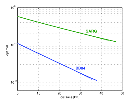
Figure 1: Lower bound on the secret-key rate per pulse and optimal $\mu$ for Poissonian sources as a function of the distance, for the BB84 and SARG protocols, when Alice and Bob share a quantum channel with perfect visibility $V=1$. The other experimental parameters are $\alpha=0.25$ dB/km, $\eta_{det}=0.1$ and $p_{d}=10^{-5}$. The thick lines are the results we obtain when Alice performs an optimal bit-wise local randomization; the thin lines are the same, without randomization ($q=0$).

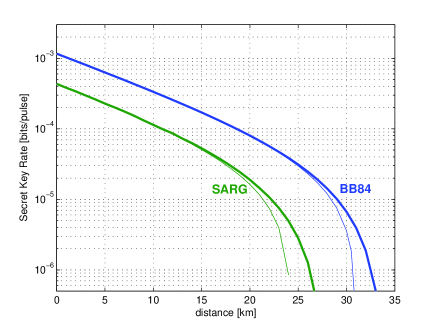
Figure 2: Same plot as in Fig. 1 (top), but for a quantum channel with non-perfect visibility, $V=0.95$.

IV.3.2 SARG

A major difference between the SARG protocol and the BB84 protocols is that Eve cannot get full information on Alice’s value even if the pulse contains two photons. In order to take this into account, we include the contribution of the two-photon components in our formula for the secret-key rate, i.e. we compute :

$$\begin{array}[]{ll}r\geq&\inf_{\{R_{1},Q_{1},R_{2},Q_{2}\}}\ R_{1}S_{1}^{\mathrm{SARG}}(Q_{1})+R_{2}S_{2}^{\mathrm{SARG}}(Q_{2})\\ &\qquad\qquad\qquad\qquad\qquad-R_{\mu}h(Q_{\mu}).\end{array}$$ (21)

In Appendix D we describe how to compute $S_{1}^{\mathrm{SARG}}(Q_{1})$ and $S_{2}^{\mathrm{SARG}}(Q_{2})$ (see also Appendix C and FuTaLo ), and we derive the following conditions for $R_{1}$, $Q_{1}$, $R_{2}$ and $Q_{2}$ to be compatible with $R_{\mu}$ and $Q_{\mu}$:

$$\begin{array}[]{rcl}R_{1}(1-Q_{1})&\leq&\frac{1}{4}p_{1}\\ R_{2}(1-Q_{2})&\leq&\frac{1}{4}p_{2}\\ R_{1}(1-Q_{1})+R_{2}(1-Q_{2})&\geq&R_{\mu}(1-Q_{\mu})\\ &&\ -\frac{1}{4}\sum_{n\geq 3}p_{n}\\ R_{1}Q_{1}+R_{2}Q_{2}&\leq&R_{\mu}Q_{\mu}.\end{array}$$ (27)

If $R_{\mu}(1-Q_{\mu})-\frac{1}{4}\sum_{n\geq 3}p_{n}>0$, one can see in (21) that Eve’s optimal choice is to set $R_{1}$ and $R_{2}$ as small as possible, and $Q_{1}$ and $Q_{2}$ as large as possible ($S_{1}^{SARG}(Q_{1})$ and $S_{1}^{SARG}(Q_{2})$ are decreasing): she should therefore set the equality in the third constraint.

However, contrary to BB84, we have not been able to give a simpler analytical expression for the infimum in (21); we therefore resort to numerical computations.

Again, in order to estimate the previous bound in a practical implementation of the protocol, we compute the typical values of the parameters $R_{\mu}$ and $Q_{\mu}$ when Alice and Bob use a Poisson source and a lossy depolarizing channel (see Appendix D):

$$\begin{array}[]{lll}R_{\mu}&=&\frac{1}{2}\big{[}1-\bar{p}_{d}^{\ 2}\ e^{-\mu\eta}+\frac{\bar{p}_{d}}{2}e^{-\mu F\eta}-\frac{\bar{p}_{d}}{2}e^{-\mu D\eta}\big{]}\\ R_{\mu}Q_{\mu}&=&\frac{1}{4}\big{[}1-\bar{p}_{d}^{\ 2}\ e^{-\mu\eta}+\bar{p}_{d}e^{-\mu F\eta}-\bar{p}_{d}e^{-\mu D\eta}\big{]}.\end{array}$$

Similarly to the BB84 protocol, inserting these values in Eq. (21), and optimizing for different distances over the mean photon number $\mu$, provides the results illustrated in Figures 1 and 2.

For $V=1$, we find an optimal $\mu$ proportional to $t^{1/2}$, and therefore our bound on the secret-key rate scales like $t^{3/2}$ (see also Koashi ), which is more efficient than for BB84 (where we had $r\propto t^{2}$). For $V=0.95$ however, we find that the SARG protocol is less efficient than the BB84, and our lower bound for the secret-key rate of SARG also scales like $t^{2}$, the same as for BB84. However, it should be noted that we determine here only lower bounds on the rates.

IV.4 Decoy states

The relevant set $\Gamma_{R_{\mu},Q_{\mu}}$ in (9) over which the infimum has to be taken to obtain the lower bound on the secret-key rate is quite big, since Alice and Bob can only estimate the total sifting and total error rate. They do neither have a good estimation of the error rates, $Q_{n}$ nor of the corresponding yields, $Y_{n}$. Hwang and Lo et. al. pointed out a method to improve the lower bound on the secret-key rate by making some additional measurements (ref_decoy ; LoMaChen see also Wang05 ). The idea of the so-called decoy states is to change the intensity of the pulses sent by Alice in order to be able to estimate more quantities. This allows them to deduce more information about the possible attack of an eavesdropper (like the estimate of the QBER does). For practical purpose one assumes that Alice is always sending weak coherent pulses, varying only the mean photon number. We will show here how this particular idea can be included in our analysis.

Let us first of all consider the case where Alice uses two different intensities, i.e., one with mean photon number $\mu_{0}$ (we call it signal pulse in the following) and the other (decoy pulse) with mean photon number $\mu_{1}$. Using more decoy states is a straightforward generalization of this case. We describe the states sent by Alice by $|\psi\rangle_{ABR_{1}R_{2}}=|\psi_{s}\rangle_{ABR_{1}}|0\rangle_{R_{2}}+|\psi_{c}\rangle_{ABR_{1}}|1\rangle_{R_{2}}$, where $|\psi_{s}\rangle_{ABR_{1}}$ ($|\psi_{c}\rangle_{ABR_{1}}$) denotes the (unnormalized) signal (decoy) pulse (see Eq. (8)). System $R_{2}$ is again some auxiliary system, introduced to keep track of the signal and decoy pulses. In this case this system is in Alice’s hands, as she chooses the intensity of the signals. Since Alice is going to measure the auxiliary system $R_{2}$ in the computational basis, we can consider the state $\sigma=p_{s}\sigma_{s}\otimes P_{|0\rangle_{R_{2}}}+(1-p_{s})\sigma_{c}\otimes P_{|1\rangle_{R_{2}}}$, where $\sigma_{s}$ ($\sigma_{c}$) are Alice and Bob’s signal (decoy) systems after Eve’s intervention, respectively. Bob’s measurement is described in the same way as before. Again, Alice and Bob can only measure the total sifting rate $R_{\mu}=\sum_{n}R_{n}=\sum_{n}p_{n}Y_{n}$ and estimate the total error rate $Q_{\mu}=\sum_{n}R_{n}Q_{n}/R_{\mu}=\sum_{n}p_{n}Y_{n}Q_{n}/R_{\mu}$. However, now they are in the position to obtain more information about their qubit pairs, as they are capable of measuring these quantities for different values of $\mu$ (recall $p_{n}=e^{-\mu}\mu^{n}/n!$), i.e. they can measure the values $R_{\mu_{0}},Q_{\mu_{0}}$ and $R_{\mu_{1}},Q_{\mu_{1}}$. We can again use (9) to compute a lower bound on the secret-key rate. In this case, the infimum is taken over the set $\Gamma_{\{R_{\mu_{i}},Q_{\mu_{i}}\}_{i}}$ of all Bell-diagonal two-qubit states of the form $p_{s}\sigma_{s}+p_{c}\sigma_{c}$, with $\sigma_{s}$ ($\sigma_{c}$) denoting the Bell-diagonal states corresponding to the signal (decoy) bits, which are compatible with all estimated total sifting rates $R_{\mu_{i}}$ and total error rates $Q_{\mu_{i}}$.

Let us now consider the case where Alice uses many different intensities for her decoy states. Due to the definition of $R_{\mu}$ it is clear that, by varying $\mu$, one can obtain information about the quantities $Y_{n}$. Knowing $Y_{n}$ and $\{Q_{\mu}\}$ one can then determine $Q_{n}$. Note that in order to determine $Y_{n}$ and $Q_{n}$ one needs infinitely many decoy intensities; however, already a small number of such decoy intensities suffices to restrict the values of $Y_{n}$ and $Q_{n}$ (see for instance Wang05 ). The results of the analysis above are illustrated in Fig. 3 and 4. In order to evaluate the lower bounds we consider the situation where Alice and Bob share a lossy depolarizing channel with visibilities $V=1$, $V=0.95$ respectively.

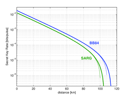
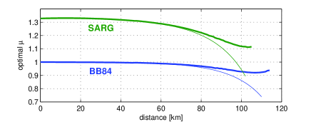
Figure 3: Lower bound on the secret-key rate per pulse and optimal $\mu$ for Poissonian sources as a function of the distance, for the BB84 and SARG protocols using decoy states, when Alice and Bob share a quantum channel with perfect visibility $V=1$. The other parameters are the same as in Fig. 1. The thick lines are the results we obtain when Alice performs an optimal bit-wise local randomization; the thin lines correspond to the protocol without randomization ($q=0$).

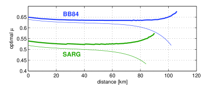
Figure 4: Same plots as in Fig. 3, but for a quantum channel with non-perfect visibility, $V=0.95$.

IV.5 Related work

In FuTaLo , a similar comparison between the BB84 and SARG protocols has been done, and lower bounds on the secret-key rates were computed. For BB84, our results are very similar to those of FuTaLo (see also LoMaChen ), but we could slightly increase the rates and the limiting distances with using the local randomization process .

For the SARG protocol, taking into account the two-photon contribution in the lower bound allows to increase the lower bound. In the case of SARG without decoy states, we could thus improve significantly the bound of FuTaLo . Our conclusion is therefore different: we find that the SARG protocol performs better than BB84 for high visibility $V\simeq 1$ (see Fig. 1). However, the SARG is more sensitive to the loss of the channel, and for $V=0.95$ for instance, BB84 is more efficient (Fig. 2).

In the case of SARG with decoy states, the two-photon contribution had already been taken into account in FuTaLo , and we again get similar results. However, we could slightly improve the rate with the improved calculation of $S_{1}^{SARG}(Q_{1})$ (see Appendix C), and with the local randomization process. Nevertheless, our conclusion is the same as in FuTaLo , namely that when decoy states are used, the SARG is outperformed by the BB84 protocol.

V Further applications, and open problems

There are still several possibilities to improve the lower bounds on the secret-key rate of QKD protocols. One way to look at this problem is to analyze the properties of the set $\Gamma$ over which one has to optimize in order to obtain the lower bound (see e.g. Eq. (3)). Concerning the single photon QKD protocols, one might try to find the conditions on the encoding (and decoding) operations which would lead to a properly restricted set $\Gamma_{Q}$, such that a high QBER can be tolerated.

In a protocol based on weak coherent pulses, it might be advantageous to take the detected double clicks into account. As mentioned above, this would (most likely) impose further restrictions on the set of possible attacks and thus result in an improvement of the secret-key rate. In addition, it would be interesting to generalize the ideas developed in this article to a scenario, where not only the intensity of light is used but where also the coherence of the light is checked (similar to the decoy states). One protocol taking this into account has for instance been proposed in COW . Another possibility is to consider protocols based on weak coherent pulses that use two-way post-processing, as studied by Lo Lo06 . We also note here that the techniques presented here can also be applied to protocols based on squeezed states.

In this work, we considered the so-called untrusted-device scenario, where the adversary might arbitrarily modify the efficiency of Bob’s detector. If one considers the reasonable situation, where Eve cannot influence Bob’s device, one might obtain larger values for the key rate.

VI Acknowledgements

The authors would like to thank Nicolas Gisin, Antonio Acin, and Valerio Scarani for helpful discussions. This project is partly supported by SECOQC and by the FWF. RR acknowledges support by HP Labs, Bristol and BK by the FWF through the Elise-Richter project.

Appendix A Proof of Lemma 1

In this appendix we prove the Lemma presented in Section III. The operator $\sigma^{\otimes n}$ is symmetric and can thus be written as $\sigma^{\otimes n}=\sum_{n^{\prime}_{1},\ldots,n^{\prime}_{4}}\mu_{n^{\prime}_{1},n^{\prime}_{2},n^{\prime}_{3},n^{\prime}_{4}}{\cal P}_{S}(P_{|\Phi_{00}\rangle}^{\otimes n^{\prime}_{1}}\otimes P_{|\Phi_{01}\rangle}^{\otimes n^{\prime}_{2}}\otimes P_{|\Phi_{10}\rangle}^{\otimes n^{\prime}_{3}}\otimes P_{|\Phi_{11}\rangle}^{\otimes n^{\prime}_{4}})$, for appropriate coefficients $\mu_{n^{\prime}_{1},n^{\prime}_{2},n^{\prime}_{3},n^{\prime}_{4}}$. Hence, with the definition $p:=\mu_{n_{1},n_{2},n_{3},n_{4}}$, we have

$$\sigma^{\otimes n}=p\rho_{n}+(1-p)\tilde{\rho}_{n}$$

where $\tilde{\rho}_{n}$ is a symmetric quantum state on $n$ subsystems. Moreover, it is easy to see that the coefficient $p$ cannot be smaller than $\frac{1}{n}$.

By linearity, we get the following expression for the state after the operation $\mathcal{E}^{\otimes\bar{n}}$ has been applied to $\sigma^{\otimes n}$:

$$\bar{\sigma}^{\otimes\bar{n}}=\mathcal{E}^{\otimes\bar{n}}(\sigma^{\otimes n})=p\mathcal{E}^{\otimes\bar{n}}(\rho_{n})+(1-p)\mathcal{E}^{\otimes\bar{n}}(\tilde{\rho}_{n})\ .$$ (28)

Because $\bar{\sigma}^{\otimes\bar{n}}$is symmetric, it can be written as $\bar{\sigma}^{\otimes\bar{n}}=\sum_{\bar{n}_{1},\ldots,\bar{n}_{4}}\bar{\mu}^{\prime}_{\bar{n}_{1},\bar{n}_{2},\bar{n}_{3},\bar{n}_{4}}{\cal P}_{S}(P_{|\Phi_{00}\rangle}^{\otimes\bar{n}_{1}}\otimes P_{|\Phi_{01}\rangle}^{\otimes\bar{n}_{2}}\otimes P_{|\Phi_{10}\rangle}^{\otimes\bar{n}_{3}}\otimes P_{|\Phi_{11}\rangle}^{\otimes\bar{n}_{4}})$, for some coefficients $\bar{\mu}^{\prime}_{\bar{n}_{1},\bar{n}_{2},\bar{n}_{3},\bar{n}_{4}}$. Furthermore, by the law of large numbers, the sum of the coefficients $\bar{\mu}^{\prime}_{\bar{n}_{1},\bar{n}_{2},\bar{n}_{3},\bar{n}_{4}}$ for tuples ${\bar{n}_{1},\bar{n}_{2},\bar{n}_{3},\bar{n}_{4}}$ which are not contained in $\mathcal{B}^{\varepsilon}(\bar{\lambda}_{1},\ldots,\bar{\lambda}_{4})$ is exponentially small, i.e.,

$$\sum_{(\bar{n}_{1},\ldots,\bar{n}_{4})\notin\mathcal{B}^{\varepsilon}(\bar{\lambda}_{1},\ldots,\bar{\lambda}_{4})}\bar{\mu}^{\prime}_{\bar{n}_{1},\bar{n}_{2},\bar{n}_{3},\bar{n}_{4}}\leq 2^{-\Theta(\bar{n}\varepsilon^{2})}\ .$$ (29)

Finally, because of (28),

$$\bar{\mu}^{\prime}_{\bar{n}_{1},\bar{n}_{2},\bar{n}_{3},\bar{n}_{4}}\geq p\cdot\bar{\mu}_{\bar{n}_{1},\bar{n}_{2},\bar{n}_{3},\bar{n}_{4}}\ ,$$

where $\bar{\mu}_{\bar{n}_{1},\bar{n}_{2},\bar{n}_{3},\bar{n}_{4}}$ are the coefficients of $\bar{\rho}_{n}$. Since $p\geq\frac{1}{n}$,

$$\bar{\mu}_{\bar{n}_{1},\bar{n}_{2},\bar{n}_{3},\bar{n}_{4}}\leq n\cdot\bar{\mu}^{\prime}_{\bar{n}_{1},\bar{n}_{2},\bar{n}_{3},\bar{n}_{4}}\ .$$

Combining this with (29), we conclude

$$\sum_{(\bar{n}_{1},\ldots,\bar{n}_{4})\notin\mathcal{B}^{\varepsilon}(\bar{\lambda}_{1},\ldots,\bar{\lambda}_{4})}\bar{\mu}_{\bar{n}_{1},\bar{n}_{2},\bar{n}_{3},\bar{n}_{4}}\leq n2^{-\Theta(\bar{n}\varepsilon^{2})}\ .$$

∎

Appendix B Advantage distillation using the XOR process

In this appendix we explain how the XOR process applied to many qubit pairs can be easily included within this formalism. Alice selects randomly a set of bits and informs Bob about this set. Then, Alice and Bob compute both the XOR of those bits and keep only the result, discarding all the others. Our goal is to find a simple description of the remaining logical bits, Eve’s system, and the classical information sent form Alice to Bob (note that Eve knows the randomly chosen set which is used by Alice and Bob). We demonstrate here how this can be achieved with the example of three qubit pairs. The idea can be easily generalized to any number of pairs.

Quantum mechanically the XOR operation can be described by a controlled-not operation, denoted by $Uc$. Three copies of the state $|\Psi\rangle_{ABE}=\sum_{i,j}\sqrt{\lambda_{i,j}}|\Phi_{i,j}\rangle_{AB}|\Phi_{i,j}\rangle_{E}$ transform, under the transformation $Uc_{A}^{3\rightarrow 1}Uc_{A}^{2\rightarrow 1}\otimes Uc_{B}^{3\rightarrow 1}Uc_{B}^{2\rightarrow 1}$ to the state

$$\sum_{i,j,k,l,m,n}\sqrt{\lambda_{i,j}\lambda_{k,l}\lambda_{m,n}}|\Phi_{i+k+m,j}\rangle_{A_{1}B_{1}}$$ (30)

$$|\Phi_{k,l+j}\rangle_{A_{2}B_{2}}|\Phi_{m,n+j}\rangle_{A_{3}B_{3}}|{\chi}_{i,j,k,l,m,n}\rangle_{E},$$

where $|{\chi}_{i,j,k,l,m,n}\rangle_{E}=|\Phi_{i,j}\rangle|\Phi_{k,l}\rangle|\Phi_{m,n}\rangle$. Since Alice and Bob are not going to use the systems $2$ and $3$ anymore, we want to consider a state that describes only Alice’s and Bob’s first systems. More importantly, we want to give Eve a purification of this state. If we would assume that Eve has a purification of the state describing systems $A_{1}$ and $B_{1}$, this would be equivalent to assume that Eve has Alice’ and Bob’s second and third pair after this transformation. It is evident that we assume then that she has more power than she actually has. In order to avoid to give her too much power we use the idea mentioned in Section II.4 (see also KrRe05 ), by considering the systems $A_{2},B_{2},A_{3},B_{3}$ as auxiliary system $R$ . For the unitary transformations, $U_{k,l,m,n}$ we choose $U_{i,j,k,l,m,n}=\sigma^{A_{1}}_{z}$ for $l+j=n+j=1$ and the identity otherwise. It can be easily verified that the state describing Alice’s and Bob’s first system is then the partial trace over $E,R$ of the state $|\tilde{\Psi}\rangle_{A_{1}B_{1}RE}=\sum_{i,j,k,l,m,n}\sqrt{\lambda_{ij}\lambda_{kl}\lambda_{mn}}$$|\Phi_{i+k+m,j+\delta_{l+j,1}\delta_{n+j,1}}\rangle_{A_{1}B_{1}}$ $|\phi_{j,k,l,m,n}\rangle_{R}|{\chi}_{i,j,k,l,m,n}\rangle_{E},$ where $|\phi_{j,k,l,m,n}\rangle_{R}$ denotes the state $|\Phi_{k,l+j}\rangle_{A_{2}B_{2}}|\Phi_{m,n+j}\rangle_{A_{3}B_{3}}$. As explained in Section II.4, providing Eve with a purification of the state that describe the systems $A_{1},B_{1}$ never underestimates her power. The eigenvalues of the two-qubit Bell-diagonal state describing Alice’s and Bob’s remaining systems, denoted by $\tilde{\lambda}_{i,j}$ are

$$\tilde{\lambda}_{i,j} = \lambda_{i,j}^{2}(\lambda_{i,j}+3\lambda_{i,j+1})+3\lambda_{i+1,j}^{2}(\lambda_{i,j}+\lambda_{i,j+1})$$

$$+ 6\lambda_{i,j}\lambda_{i+1,j}\lambda_{i+1,j+1}.$$

The intuition for this choice of unitary transformations is the following. The state $|\Psi\rangle_{ABE}$ under consideration is supposed to lead to a secret-bit. Thus, the coefficients $\lambda_{i,j}$ are such that it is very likely that if both, $l+j=1$ and $n+j=1$ then $j=1$, which means that within the remaining qubit-pair there is a phase-flip error. The unitaries are chosen such that this error is corrected.

Using the new eigenvalues of the state describing Alice’ and Bob’s remaining bits, it is straightforward to compute the lower bound on the secret-key rate (Eq. (3)).

Appendix C An improved analysis of the SARG protocol with single photons

In the SARG protocol the bit value $0$ ($1$) is encoded in the $z$-basis ($x$-basis) respectively. During the sifting phase Alice announces a set containing two states, the one which she sent and one in the other basis. There are $4$ different encoding and decoding operators. For instance $A_{1}=|0\rangle\langle 0_{z}|+|1\rangle\langle 0_{x}|$ and $B_{1}=|0\rangle\langle 1_{x}|+|1\rangle\langle 1_{z}|$ describe the situation where Alice sends on of the two states $\{|0_{z}\rangle,|0_{x}\rangle\}$ and tells Bob that the sent state is within this set. Let us for the moment consider a single qubit sent by Alice (for more details see BrGi05 ). The state shared by Alice, Bob, and Eve after the sifting is given by $|\chi\rangle_{ABER_{1}}=\sum_{j}A_{j}\otimes B_{j}|\Psi\rangle_{ABE}|j\rangle_{R_{1}}$, where $|\Psi\rangle_{ABE}$ is the state shared by Alice, Bob, and Eve after Eve s intervention. Now, we apply some symmetrization to the state, which does not change any security consideration, as explained in Section II. Let us consider the state $|\tilde{\chi}\rangle_{ABER_{1}R_{2}}=|\chi\rangle_{ABER_{1}}|0\rangle_{R_{2}}+\sigma_{z}^{A}\otimes\sigma_{z}^{B}|\chi\rangle_{ABER_{1}}|1\rangle_{R_{2}}$. It is straightforward to show that the reduced state describing Alice’ and Bob’s system is equal to $\tilde{\mathcal{D}}_{2}{\mathcal{D}_{1}[\mathcal{D}_{2}(\rho_{0})]}$, with $\rho_{0}=\mathrm{tr}_{E}(P_{\Psi})$. Here, $\tilde{\mathcal{D}}_{2}(\rho)=1/2(\rho+\sigma_{z}\otimes\sigma_{z}\rho\sigma_{z}\otimes\sigma_{z})$, $\mathcal{D}_{1}(\rho)=\sum_{j}A_{j}\otimes B_{j}\rho A_{j}^{\dagger}\otimes B_{j}^{\dagger}$ is given by the protocol and $\mathcal{D}_{2}$ denotes the depolarizing map, i.e. $\mathcal{D}_{2}(\rho)=1/4(\rho+\sigma_{x}\otimes\sigma_{x}\rho\sigma_{x}\otimes\sigma_{x}+\sigma_{y}\otimes\sigma_{y}\rho\sigma_{y}\otimes\sigma_{y}+\sigma_{z}\otimes\sigma_{z}\rho\sigma_{z}\otimes\sigma_{z})$. Furthermore, the action of $\mathcal{D}_{1}$ on a Bell-diagonal state is the same as $A_{1}\otimes B_{1}$ on that state. Thus, we only need to consider the situation where Eve has a purification of the state $\mathcal{D}_{2}(\rho_{0})$, i.e. the state before the action of $\mathcal{D}_{1}$ and $\tilde{\mathcal{D}}_{2}$. Using the results of KrRe05 ; ReKr05 this implies that the state we have to use in order to compute the lower bound on the secret-key rate is $\rho_{ABE}=\tilde{\mathcal{D}}_{2}^{AB}(P_{A_{1}\otimes B_{1}|\Phi\rangle_{ABE}})$, where $|\Phi\rangle_{ABE}=\sqrt{\lambda_{00}}|\Phi_{00}\rangle_{AB}|\Phi_{00}\rangle_{E}+\sqrt{\lambda_{01}}|\Phi_{01}\rangle_{AB}|\Phi_{01}\rangle_{E}+\sqrt{\lambda_{10}}|\Phi_{10}\rangle_{AB}|\Phi_{10}\rangle_{E}+\sqrt{\lambda_{11}}|\Phi_{11}\rangle_{AB}|\Phi_{11}\rangle_{E}$, i.e a purification of the Bell-diagonal state $\mathcal{D}_{2}(\rho_{0})$.

Using this description it is straightforward to compute the state describing Alice’ and Bob’s system, which is, in contrast to former considerations, no longer Bell-diagonal. In the following we consider the situation where Bob accepts only if the probability for him to obtain the bit values $0$ is the same as detecting $1$. This is a first step in the parameter estimation. Note that this condition imposes $\lambda_{01}=\lambda_{10}$. The QBER, $Q$, can be easily determined and one finds $Q=(\lambda_{01}+\lambda_{11})/(1/2+\lambda_{01}+\lambda_{11})$. Using the normalization condition we find that the coefficients in the state $|\Phi\rangle_{ABE}$ are given by: $\lambda_{00}=1-Q/(1-Q)+\lambda_{11},\lambda_{01}=Q/(2(1-Q))-\lambda_{11},\lambda_{10}=\lambda_{01}$. Thus, for a fixed QBER there is only one parameter, $\lambda_{11}\in[0,Q/(2(1-Q))]$, over which one needs to minimize to obtain the lower bound on the secret-key rate given in formula Eq. (4). Without the local randomization one finds that the lower bound on the secret-key rate is positive as long as $Q\leq 0.1167$. Including the local randomization allows to increase the tolerable QBER to $0.1308$ compared to the previously known bounds of $0.0968$ without and $0.1095$ with local randomization, respectively BrGi05 .

Appendix D Calculations related to the analysis of protocols based on coherent pulses

This appendix contains some calculations related to the evaluation of the lower bound (9) on the secret-key rate for the BB84 and SARG protocols with weak coherent pulses (see Section IV).

For this purpose, we first compute the infimum $S_{n}(Q_{n}):=\inf_{\sigma_{n}\in\Gamma_{Q_{n}}}S(X|E,n)$ for any given $Q_{n}$, and then optimize (from Eve’s point of view) over the parameters $R_{n},Q_{n}$. These parameters must be compatible with the measurable quantities $R_{\mu},Q_{\mu}$: in the case of protocols which do not use decoy states, this leads to particular constraints for each protocol, which we derive here. (Note that for protocols with decoy states, Alice and Bob can estimate all rates $R_{n},Q_{n}$: Eve can no longer optimize over these parameters.)

Recall that we work in the untrusted device scenario, where Eve has full control over Bob’s detectors. Dark counts do not occur, and therefore $R_{0}=0$, as Eve should obviously not send any photon to Bob when she receives an empty pulse from Alice. Moreover, we consider protocols where Bob treats all double clicks as if only one randomly chosen detector clicked.

In a second step, in order to give estimations of our bounds, we compute the typical values of the yields and error rates if no adversary is present, i.e., if the channel between Alice and Bob is a depolarizing channel with fidelity F (or disturbance $D=1-F$) and with a transmission factor $t$. In addition, we suppose in that case that Bob’s detectors have an efficiency $\eta_{det}$ and a probability of dark counts $p_{d}$. We will use the notations $\eta=t\eta_{det}$ for the overall transmission factor and $\bar{p}_{d}=1-p_{d}$.

D.1 BB84 protocol

D.1.1 Eve’s uncertainty on the one-photon pulses

For BB84, the set $\Gamma_{Q_{1}}$ contains all states with diagonal entries (in the Bell basis) $\lambda_{00}=1-2Q_{1}+\lambda_{11}$ and $\lambda_{01}=\lambda_{10}=Q_{1}-\lambda_{11}$, for any $\lambda_{11}\in[0,Q_{1}]$ KrRe05 ; ReKr05 .

One can easily prove that $S(X|E,n=1)$ takes its minimum when $\lambda_{1,1}=Q_{1}^{2}$. Then, a straightforward calculation shows that $S_{1}^{BB84}(Q_{1})=\inf_{\sigma_{1}\in\Gamma_{Q_{1}}}S(X|E,n=1)=1-h(Q_{1})$. Note that $S_{1}^{BB84}(Q_{1})$ is decreasing for $0\leq Q_{1}\leq 1/2$: as expected, the higher the error Eve introduces, the more she reduces her uncertainty.

D.1.2 Constraints on the yields and error rates

In the BB84 protocol, the probability that Alice and Bob choose the same basis for their preparation and measurement respectively is $1/2$ (this is the sifting factor). Therefore we have $Y_{n}\leq\frac{1}{2}$ for all $n$, which implies the following bounds:

$$R_{1} = p_{1}Y_{1}\leq\frac{1}{2}p_{1}$$ (32)

$$R_{1} = R_{\mu}-\sum_{n\geq 2}p_{n}Y_{n}\geq R_{\mu}-\frac{1}{2}\sum_{n\geq 2}p_{n}.$$ (33)

These are the first two constraints announced in (17). The third constraint follows from the definition of $Q_{\mu}$, $R_{\mu}Q_{\mu}=\sum_{n}R_{n}Q_{n}$.

D.1.3 Yields and error rates for depolarizing channels

When implementing the BB84 protocol, Alice and Bob would estimate the quantities $Q_{\mu}$, $R_{\mu}$ and then compute the rate as explained above. In order to get an idea how good the obtained bounds on the rate are we evaluate here these quantities for the situation where there is no Eve present and Alice and Bob share a lossy depolarizing channel.

In BB84, when Alice sends $n$ photons, the probability that Bob chooses the same basis as Alice and gets a single or a double click is :

$$\begin{array}[]{lll}Y_{n}&=&\frac{1}{2}\big{[}1-\bar{p}_{d}^{\ 2}(1-\eta)^{n}\big{]}\end{array}$$

Bob gets a wrong bit if only the wrong detector clicks, or if the two detectors click, but he randomly chooses a wrong bit. This happens with probability :

$$\begin{array}[]{lll}Y_{n}Q_{n}&=&\frac{1}{2}\sum_{k=0}^{n}\mathrm{C}_{n}^{k}F^{k}D^{n-k}\Big{[}[\bar{p}_{d}(1-\eta)^{k}][1-\bar{p}_{d}(1-\eta)^{n-k}]\\ &&\qquad\qquad+\frac{1}{2}[1-\bar{p}_{d}(1-\eta)^{k}][1-\bar{p}_{d}(1-\eta)^{n-k}]\Big{]}\\ &=&\frac{1}{4}\big{[}1+\bar{p}_{d}(1-F\eta)^{n}-\bar{p}_{d}(1-D\eta)^{n}-\bar{p}_{d}^{\ 2}(1-\eta)^{n}\big{]}\end{array}$$

When Alice uses a Poissonian source (i.e. $p_{n}=\frac{\mu^{n}}{n!}e^{-\mu}$), the overall yield and error rate are then

$$\begin{array}[]{lll}R_{\mu}&=&\frac{1}{2}\big{[}1-\bar{p}_{d}^{\ 2}\ e^{-\mu\eta}\big{]}\\ R_{\mu}Q_{\mu}&=&\frac{1}{4}\big{[}1+\bar{p}_{d}e^{-\mu F\eta}-\bar{p}_{d}e^{-\mu D\eta}-\bar{p}_{d}^{\ 2}\ e^{-\mu\eta}\big{]}.\end{array}$$

D.2 SARG protocol

D.2.1 Eve’s uncertainty on the one-photon pulses

In order to compute Eve’s uncertainty on the one-photon pulses, we use the method presented in Appendix C. We don’t have an analytical expression for $S_{1}^{SARG}(Q_{1})=\inf_{\sigma_{1}\in\Gamma_{Q_{1}}}S(X|E,n=1)$, but we compute it numerically. Note that we find $S_{1}^{SARG}(Q_{1})$ is decreasing only for $0\leq Q_{1}\lesssim 0.338$, and does not reach zero.

D.2.2 Eve’s uncertainty on the two-photon pulses

We follow the calculations of FuTaLo to compute Eve’s uncertainty on the two-photon pulses. The set $\Gamma_{Q_{2}}$ contains all states with the following diagonal entries (in the Bell basis)

$$\begin{array}[]{l}\lambda_{00}=1-Q_{2}-\lambda_{01}\\ \lambda_{10}=Q_{2}-\lambda_{11}\\ \lambda_{01}+\lambda_{11}\leq xQ_{2}+g(x),\forall x\end{array}$$ (37)

where $g(x)=\frac{1}{6}(3-2x+\sqrt{6-6\sqrt{2}x+4x^{2}})$ FuTaLo . When minimizing $xQ_{2}+g(x)$ over $x$, we get

$$\begin{array}[]{l}\lambda_{00}=1-Q_{2}-\lambda_{01}\\ \lambda_{10}=Q_{2}-\lambda_{11}\\ \lambda_{01}+\lambda_{11}\leq B(Q_{2})\end{array}$$ (41)

where $B(Q_{2})=\frac{1}{2}+\frac{1}{2}\sqrt{Q_{2}(1-\frac{3Q_{2}}{2})}-\frac{\sqrt{2}}{4}(1-3Q_{2})$.

One can show that for $Q_{2}\leq\frac{1}{6}$, $B(Q_{2})\leq\frac{1}{2}$ and the optimal choice of the parameters $\lambda_{ij}$ for Eve is $\lambda_{01}+\lambda_{11}=B(Q_{2})$ (i.e. Eve should make the phase error as high as possible, up to $\frac{1}{2}$), and $\lambda_{11}=Q_{2}B(Q_{2})$. Then, a straightforward calculation gives $S_{2}^{SARG}(Q_{2})=\inf_{\sigma_{2}\in\Gamma_{Q_{2}}}S(X|E,n=2)=1-h(B(Q_{2}))$. Note that $S_{2}^{SARG}(Q_{2})$ is decreasing for $0\leq Q_{2}\leq\frac{1}{6}$, and $S_{2}^{SARG}(\frac{1}{6})=0$.

D.2.3 Constraints on the yields and error rates

In the case of SARG, because of the non orthogonality of the quantum states that are used to encode the classical bit values, it is a little bit more tricky to find the constraints that the yields and error rates must satisfy. Here, we will derive a constraint on the yields without errors (or probability that Bob gets a right conclusive result), i.e., on $p_{\mathrm{right}}=Y_{n}(1-Q_{n})$ (for any $n\in\mathbb{N}$).

To this aim, let’s suppose in a first step that Alice sends photons in the state $|+z\rangle$, that Eve attacks the pulse and decides either to forward one photon to Bob in the state $\rho_{B}$, or to block the pulse. In this case, Bob gets a right conclusive result if (i) Alice announces the set $\{|+z\rangle,|+x\rangle\}$ (which she does with probability 1/2), Bob chooses to measure $\sigma_{x}$ (probability 1/2) and (only) the detector corresponding to $|-x\rangle$ clicks ; or (ii) Alice announces the set $\{|+z\rangle,|-x\rangle\}$, Bob chooses to measure $\sigma_{x}$, and the detector corresponding to $|+x\rangle$ clicks. Therefore, Bob’s probability to get a right conclusive result when Alice sends $|+z\rangle$ is bounded by:

$$p_{\mathrm{right}|+z} \leq \frac{1}{4}\langle-x|\rho_{B}|-x\rangle+\frac{1}{4}\langle+x|\rho_{B}|+x\rangle$$ (42)

$$\leq \frac{1}{4}\ Tr(\rho_{B})=\frac{1}{4}.$$ (43)

This result actually does not depend on the state sent by Alice, and we therefore have

$$p_{\mathrm{right}}=Y_{n}(1-Q_{n})\leq\frac{1}{4}.$$ (44)

The first three constraints announced in (27) then follow :

$$R_{1}(1-Q_{1}) \leq \frac{1}{4}p_{1}$$ (45)

$$R_{2}(1-Q_{2}) \leq \frac{1}{4}p_{2}$$ (46)

$$R_{1}(1-Q_{1})+R_{2}(1-Q_{2}) \geq R_{\mu}(1-Q_{\mu})-$$ (48)

$$\ -\frac{1}{4}\sum_{n\geq 3}p_{n}$$

As before, the last constraint follows from the definition of $Q_{\mu}$.

D.2.4 Yields and error rates for depolarizing channels

As for the BB84–protocol, we evaluate here the lower bound on the secret key rate for the situation where there is no Eve present and Alice and Bob share a lossy depolarizing channel, in order to get an idea of how good the obtained bounds on the rate are.

In order to calculate the yields and error rates for the SARG protocol, let’s suppose that Alice sends $n$ photons in the state $|+z\rangle$, and announces $\{|+z\rangle,|+x\rangle\}$. By symmetry, the following still holds for any state sent by Alice, and any announcement. Similar calculations can be found in BrGi05 .

If Bob measures $\sigma_{z}$, he gets a (wrong) conclusive click on the detector corresponding to $|-z\rangle$, or a double click with probabilities:

$$\begin{array}[]{lll}p_{|-z\rangle|z}&=&\sum_{k=0}^{n}\mathrm{C}_{n}^{k}F^{k}D^{n-k}[\bar{p}_{d}(1-\eta)^{k}][1-\bar{p}_{d}(1-\eta)^{n-k}]\\ &=&\bar{p}_{d}(1-F\eta)^{n}-\bar{p}_{d}^{\ 2}(1-\eta)^{n}\\ p_{2clicks|z}&=&1-\bar{p}_{d}(1-F\eta)^{n}-\bar{p}_{d}(1-D\eta)^{n}+\bar{p}_{d}^{\ 2}(1-\eta)^{n}\end{array}$$

Similarly, if Bob now measures $\sigma_{x}$, he gets a (right) conclusive click on the detector corresponding to $|-x\rangle$, or a double click with probabilities:

$$\begin{array}[]{lll}p_{|-x\rangle|x}&=&\bar{p}_{d}(1-\frac{\eta}{2})^{n}-\bar{p}_{d}^{\ 2}(1-\eta)^{n}\\ p_{2clicks|x}&=&1-2\bar{p}_{d}(1-\frac{\eta}{2})^{n}+\bar{p}_{d}^{\ 2}(1-\eta)^{n}\end{array}$$

Since Bob randomly chooses the basis he measures, with equal probabilities, and since he randomly chooses one outcome in the case of double clicks (conclusive or not), then the probability that Bob’s result is conclusive when Alice sends $n$ photons is $Y_{n}=\frac{1}{2}\big{(}p_{|-z\rangle|z}+\frac{1}{2}p_{2clicks|z}\big{)}+\frac{1}{2}\big{(}p_{|-x\rangle|x}+\frac{1}{2}p_{2clicks|x}\big{)}$, and the error rate on these pulses is $Y_{n}Q_{n}=\frac{1}{2}\big{(}p_{|-z\rangle|z}+\frac{1}{2}p_{2clicks|z}\big{)}$. We find:

$$\begin{array}[]{lll}Y_{n}&=&\frac{1}{2}\big{[}1+\frac{\bar{p}_{d}}{2}(1-F\eta)^{n}-\frac{\bar{p}_{d}}{2}(1-D\eta)^{n}-\bar{p}_{d}^{\ 2}(1-\eta)^{n}\big{]}\\ Y_{n}Q_{n}&=&\frac{1}{4}\big{[}1+\bar{p}_{d}(1-F\eta)^{n}-\bar{p}_{d}(1-D\eta)^{n}-\bar{p}_{d}^{\ 2}(1-\eta)^{n}\big{]}\end{array}$$

For a Poissonian source, the overall yield and error rate are then

$$\begin{array}[]{lll}R_{\mu}&=&\frac{1}{2}\big{[}1+\frac{\bar{p}_{d}}{2}e^{-\mu F\eta}-\frac{\bar{p}_{d}}{2}e^{-\mu D\eta}-\bar{p}_{d}^{\ 2}\ e^{-\mu\eta}\big{]}\\ R_{\mu}Q_{\mu}&=&\frac{1}{4}\big{[}1+\bar{p}_{d}e^{-\mu F\eta}-\bar{p}_{d}e^{-\mu D\eta}-\bar{p}_{d}^{\ 2}\ e^{-\mu\eta}\big{]}.\end{array}$$

References

- (1) N. Gisin, G. Ribordy, W. Tittel, and H. Zbinden, Reviews of Modern Physics, 74, 145 (2002).
- (2) http://www.idquantique.com, http://www.magiqtech.com.
- (3) N. Gisin, G. Ribordy, H. Zbinden, D. Stucki, N. Brunner, V. Scarani, quant-ph/0411022 (2004); D. Stucki, N. Brunner, N. Gisin, V. Scarani, H. Zbinden, Appl. Phys. Lett. 87, 194108 (2005).
- (4) K. Inoue, E. Waks, Y. Yamamoto, Phys. Rev. A 68, 022317 (2003).
- (5) G. Brassard and L. Salvail, Workshop on the theory and application of cryptographic techniques on Advances in cryptology, pp. 410–423 (1994).
- (6) B. Kraus, N. Gisin, and R. Renner Phys. Rev. Lett. 95, 080501 (2005).
- (7) R. Renner, N. Gisin, and B. Kraus Phys. Rev. A 72, 012332 (2005).
- (8) P. W. Shor and J. Preskill, Phys. Rev. Lett. 85, 441, (2000).
- (9) C. H. Bennett and G. Brassard, in Proceedings of International Conference on Computer Systems and Signal Processing, p. 175 (1984).
- (10) D. Bruss, Phys. Rev. Lett. 81, 3018 (1998); H. Bechmann-Pasquinucci, N. Gisin, Phys. Rev A, 59, 4238 (1999).
- (11) C. H. Bennett, Phys. Rev. Lett. 68, 3121 (1992).
- (12) V. Scarani, A. Acin, G. Ribordy, and N. Gisin, Phys. Rev. Lett. 92, p. 057901 (2004).
- (13) C. Branciard, N. Gisin, B. Kraus, V. Scarani Phys. Rev. A 72, 032301 (2005).
- (14) H.-K. Lo, Quant. Info. Comp., 1, No. 2, p. 81–94 (2001).
- (15) H.-K. Lo, Quant. Info. Comp., 5, No. 4/5, pp. 413–418 (2005).
- (16) G. Smith, J. M. Renes, J. A. Smolin, quant-ph/0607018 (2006).
- (17) J. M. Renes, G. Smith, quant-ph/0603262 (2006).
- (18) U. Maurer, IEEE Transaction on Information Theory, 39, 733–742 (1993).
- (19) D. Gottesman and H.-K. Lo, IEEE Transactions on Information Theory, 49, 457 (2003).
- (20) H. F. Chau, Phys. Rev. A 66, 060302 (2002).
- (21) R. Renner, Security of Quantum Key Distribution, PhD thesis, ETH (2005), available at: http://arxiv.org/abs/quant-ph/0512258.
- (22) A. Acin, J. Bae, E. Bagan, M. Baig, Ll. Masanes, R. Munoz-Tapia, Phys. Rev. A 73, 012327 (2006).
- (23) J. Bae and A. Acin, quant-ph/0610048 (2006).
- (24) H.-K. Lo, X. Ma, K. Chen, Phys. Rev. Lett. 94, 230504 (2005).
- (25) C.-H. F. Fung, K. Tamaki, H.-K. Lo, Phys. Rev. A 73, 012337 (2006).
- (26) H. Inamori, N. Lutkenhaus, D. Mayers, quant-ph/0107017 (2001).
- (27) D. Gottesman, H.-K. Lo, N. Lutkenhaus, J. Preskill, Quantum Info. and Comp., 4, No.5 pp. 325–360 (2004).
- (28) W.-Y. Hwang, Phys. Rev. Lett. 91, 057901 (2003).
- (29) X.-B. Wang, Phys. Rev. Lett. 94, 230503 (2005).
- (30) X. Ma, C-H F. Fung, F. Dupuis, K. Chen, K. Tamaki, H-K Lo, Phys. Rev. A 74, 032330 (2006).
- (31) M. Koashi, quant-ph/0507154 (2005).