Simultaneous creations of discrete-variable entangle state and single-photon-added coherent state

Abstract

The single-photon-added coherent state (SPACS), as an intermediate classical-to-purely-quantum state, was first realized recently by Zavatta $et~{}al.$ (Science 306, 660 (2004)). We show here that the success probability of their SPACS generation can be enhanced by a simple method which leads to simultaneous creations of a discrete-variable entangled state and a SPACS or even a hybrid-variable entangled SPACS in two different channels. The impacts of the input thermal noise are also analyzed.

OCIS codes: 270.0270, 190.4410, 270.1670, 230.4320

The preparations of a nonclassical quantum state are essential in current quantum information science. Many schemes have been formulated in the past decade based on the nonlinear mediums or the technique of conditional measurements 1 ; 2 ; 3 ; 4 ; 5 ; 6 ; 7 ; 8 . For example, Sanders proposed a concept of entangled coherent state (ECS) by using a nonlinear interferometer 6 . Dakna $et~{}al.$ used a conditional measurement on the beam-splitters (BS) to create several kinds of nonclassical states 7 . Agarwal and Tara presented a hybrid nonclassical state called a photon-added coherent state (PACS) which exhibits an intermediate property between a classical coherent state (CS) and a purely quantum Fock state (FS) 8 . Recently, by using a type-I beta-barium borate(BBO)crystal, a single-photon detector (SPD) and a balanced homodyne detector, Zavatta $et~{}al.$ experimentally created a single-photon-added coherent state (SPACS) which allowed them to first visualize the classical-to-quantum transition process 9 . By applying the Sanders ECS, a feasible scheme was proposed to create even an entangled SPACS (ESPACS) from which one achieves a type-II hybrid entanglement of the quantum FS and the classical CS [5]. Then it is clear that, for the purpose of practical applications, the rare success probability of the SPACS generation in the experiment of Zavatta $et~{}al.$ 9 should be largely improved. In this paper, by directly combining many parametric amplifiers in the original scheme of Zavatta $et~{}al.$ 9 , a simple but efficient method is presented to significantly improve the success probability of their SPACS generation, which is made possible by simultaneously preparing a discrete-variable entangled $W$ state 10 and a SPACS (hybrid-variable quantum state) in two different channels.

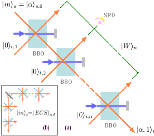
Figure 1: (Color online) Schematic diagram to simultaneously create the discrete-variable entangled $W$ state and the SPACS in two different channels. The input signal is in (a) a classical CS 9 or (b) an ECS 5 ; 6 .

The PACS $|\alpha,m\rangle$, firstly introduced by Agarwal and Tara 8 , is defined as

$$|\alpha,m\rangle=\frac{\hat{a}^{{\dagger}m}|\alpha\rangle}{[m!L_{m}(-|\alpha|^{2})]^{1/2}},$$ (1)

where $\hat{a}$ $(\hat{a}^{{\dagger}})$ is the photon annihilation (creation) operator and $L_{m}(x)$ is the Laguerre polynomial ($m$ is an integer), $L_{m}(x)=\sum_{n=0}^{m}\frac{(-1)^{n}x^{n}m!}{(n!)^{2}(m-n)!}$. Obviously, for $\alpha$ (or $m$) $\rightarrow 0$, $|\alpha,m\rangle$ reduces to the FS (CS). The interesting properties of PACS, as an intermediate classical-to-quantum state, was studied in Ref. 8 . We note that another different intermediate state called the displaced FS: $|DFS\rangle=D(\alpha)|n\rangle=\exp(\hat{a}^{{\dagger}}\alpha-\hat{a}\alpha^{*})|n\rangle$, is obtained by acting upon the FS with the displacement operators 4 . The PACS is, however, obtained via the successive one-photon excitations on a classical CS light.

Now we consider the parametric down-conversion process (type-I BBO crystal) in which one photon incident on the dielectric with $\chi^{2}$ nonlinearity breaks up into two new photons of lower frequencies. In the steady state, we always have $\omega_{p}=\omega_{s}+\omega_{i}$, where $\omega_{p}$ is the pump frequency, and $\omega_{s}$ or $\omega_{i}$ is the signal or idler frequency. Under the phase matching condition, the wave vectors of the pump, signal and idler photons are related by $\vec{k}_{p}=\vec{k}_{s}+\vec{k}_{i}$ (momentum conservation). The signal and idler photons appear simultaneously within the resolving time of the detectors and the associated electronics 11 . The Hamiltonian in the interaction picture is then: $\hat{H}_{I}=\hbar g[\hat{a}_{s}^{{\dagger}}\hat{a}_{i}^{{\dagger}}\hat{a}_{p}+\hat{a}_{s}\hat{a}_{i}\hat{a}_{p}^{{\dagger}}],$ where the real coupling constant $g$ contains the nonlinear susceptibility $\chi^{2}$. The free-motion parts of the total Hamiltonian commute with $\hat{H}_{I}$. Thereby one pump photon is converted into one signal and one idler photon.

We consider for simplicity the signal and idler lights with a same polarization and the well-defined directions, and an incident intense pump for which the quantum operator $\hat{a}_{0}$ can be treated classically as $\hat{a}_{0}\rightarrow iV$. Then for an input CS: $|\psi(0)\rangle_{1}=|\alpha\rangle_{s}|0\rangle_{i}$, the output state after an interaction time $t$ with one nonlinear crystal evolves into: $|\psi(t)\rangle_{1}=\exp[-i\hat{H}_{I}t/\hbar]|\psi(0)\rangle_{1}=\exp[\lambda(\hat{a}_{s}^{{\dagger}}\hat{a}_{i}^{{\dagger}}-\hat{a}_{s}\hat{a}_{i})]|\psi(0)\rangle_{1},$ with an effective interaction time $\lambda=Vgt$. For short times $t$ compared with the average time interval between the successive down-conversions, by expanding the exponential we have ($\lambda\ll 1$)

$$|\psi(t)\rangle_{1}\approx|\alpha\rangle_{s}|0\rangle_{i}+\lambda|\alpha,1\rangle_{s}|1\rangle_{i}+\frac{\lambda^{2}}{2}(\hat{a}_{s}^{{\dagger}}\hat{a}_{i}^{{\dagger}}\hat{a}_{s}^{{\dagger}}\hat{a}_{i}^{{\dagger}}-\hat{a}_{s}\hat{a}_{i}\hat{a}_{s}^{{\dagger}}\hat{a}_{i}^{{\dagger}})|\alpha\rangle_{s}|0\rangle_{i}.$$ (2)

Due to $\lambda\ll 1$, we can select the first two terms as the output state, i.e., $|\psi(t)\rangle_{1}\approx|\alpha\rangle_{s}|0\rangle_{i}+\lambda|\alpha,1\rangle_{s}|1\rangle_{i}$. Thus the signal channel mostly contains the input CS, except for the few cases when a single photon is detected in the output idler. These $rare$ events stimulate one-photon emission into the CS and then generate a SPACS in the output signal with a success probability being proportional to $p_{1}^{1}=|\lambda|^{2}(1+|\alpha|^{2})$. As in the experiment of Zavatta $et~{}al.$ 9 , the one-photon excitation is selected to avoid the higher-order ones which cannot be discriminated by the SPD with finite efficiency.

As shown in Fig. 1(a), we consider the direct combination of a series of two or more (say, $N$) identical optical parametric amplifiers by assuming for simplicity the same low-gain ($g_{j}=g$, $j=1,2,...N$) and the same classical pumps. For an input CS in the signal and a vacuum in all the idlers, i.e.,

$$|\psi(0)\rangle_{N}=|\alpha\rangle_{s,0}|0\rangle_{i,1}|0\rangle_{i,2}\ldots|0\rangle_{i,N},$$ (3)

the output state is a $(N+1)$-body hybrid entangled state which reads:

$$|\psi(t)\rangle_{N}=\prod_{j=1}^{N}\exp[-i\hat{H}_{jI}t/\hbar]|\psi(0)\rangle_{N},$$ (4)

where $\hat{H}_{jI}=i\hbar gV[\hat{a}_{s,j}^{{\dagger}}\hat{a}_{i,j}^{{\dagger}}-\hat{a}_{s,j}\hat{a}_{i,j}]$. Based on the conditional detections of SPDs in the idlers, the PACS $|\alpha,m\rangle$ is generated with the success probability being proportional to $p_{N}^{m}=N|\lambda^{m}|^{2}m!L_{m}(-|\alpha|^{2})$ ($m\leq N$). Clearly, for $m=1$ (SPACS), we have a simple relation: $p_{N}^{1}=Np_{1}^{1}$, which means that, at least under the ideal conditions, the success probability of the optical SPACS generation can be improved $N$ times in comparison with the original scheme of Zavatta $et~{}al.$ 9 .

This significant improvement of the SPACS generation has a simple physical explanation, i.e., the formation of the $N$-qubit $W$ entangled state in the idlers. In fact, it is easy to verify that, when a SPACS is achieved in the output signal, one has the following state in the idlers

$$|\psi(t)\rangle_{N}^{W}=\frac{1}{\sqrt{N}}(|1\underbrace{00\cdots 0}_{N-1}\rangle+|01\underbrace{00\cdots 0}_{N-2}\rangle+\cdots+|\underbrace{00\cdots 0}_{N-1}1\rangle).$$ (5)

This means that, as long as anyone of the $N$ detectors captures one photon, a SPACS can be achieved! In other words, an observation of the SPACS cannot tell us which one of the $N$ detectors was hit by a single photon. It is this quantum $indistinguishability$ which leads to the simultaneous (and enhanced) generation of the discrete-variable entangle $W$ state and the SPACS in two different channels.

Example-1: $N=2$. For an input state: $|\psi(0)\rangle_{2}=|\alpha\rangle_{s,0}|0\rangle_{i,1}|0\rangle_{i,2}$, the output state of the system is

$$|\psi(t)\rangle_{2}\approx|\alpha\rangle_{s}|0\rangle_{i,1}|0\rangle_{i,2}+\lambda|\alpha,1\rangle_{s}|EPR\rangle_{2}+\lambda^{2}|\alpha,2\rangle_{s}|1\rangle_{i,1}|1\rangle_{i,2},$$ (6)

where we denote $|EPR\rangle_{2}=|1\rangle_{i,1}|0\rangle_{i,2}+|0\rangle_{i,1}|1\rangle_{i,2}$. Obviously, due to $\lambda\ll 1$, we can select the first two terms as the output state and the SPACS is created in the output signal with a success probability being proportional to: $p_{2}^{1}=2p_{1}^{1}=2|\lambda|^{2}(1+|\alpha|^{2})$. In short, via the conditional SPDs technique of Zavatta $et~{}al.$ 9 , the probabilistic SPACS generation is enhanced $2$ times by simultaneously creating an EPR-type maximally entangled state and the SPACS in two different channels.

Example-2: $N=3$. Still for a classical CS input signal, we achieve the output state of the system:

$$|\psi(t)\rangle_{3}\approx|\alpha\rangle_{s}|0\rangle_{i,1}|0\rangle_{i,2}|0\rangle_{i,3}+\lambda|\alpha,1\rangle_{s}|W\rangle_{3}+\lambda^{2}|\alpha,2\rangle_{s}|II\rangle_{3}+\lambda^{3}|\alpha,3\rangle_{s}|1\rangle_{i,1}|1\rangle_{i,2}|1\rangle_{i,3},$$ (7)

with the $3$-body entangled states $|W\rangle_{3}=|1\rangle_{i,1}|0\rangle_{i,2}|0\rangle_{i,3}+|0\rangle_{i,1}|1\rangle_{i,2}|0\rangle_{i,3}+|0\rangle_{i,1}|0\rangle_{i,2}|1\rangle_{i,3}$ and $|II\rangle_{3}=|1\rangle_{i,1}|1\rangle_{i,2}|0\rangle_{i,3}+|0\rangle_{i,1}|1\rangle_{i,2}|1\rangle_{i,3}+|1\rangle_{i,1}|0\rangle_{i,2}|1\rangle_{i,3}$. Obviously, due to $\lambda\ll 1$, we still can select the first two terms as the output state and the SPACS is created with a success probability being proportional to: $p_{3}^{1}=3p_{1}^{1}=3|\lambda|^{2}(1+|\alpha|^{2})$, which is made possible by simultaneously creating the $3$-body $W$-type maximally entangled state and the SPACS in two different channels (see also the Eq. (5)).

As a practical realization, the $N$ idlers can be connected by a multi-port optical fiber to one SPD since in all of the $N$ idlers there is maximally one photon to be detected for $\lambda\ll 1$. We note that, although it is difficult to achieve a large $N$ with the condition of a strong strength for all the pumps if one uses some beam-splitting technique on one strong pump laser beam 13 , this method still can be useful due to the extreme difficulty to achieve a large nonlinear susceptibility in the ordinary nonlinear optics mediums 1 . To further improve the success probability of the SPACS generation, one can even consider, e.g., the complex technique of electromagnetically induced transparency (EIT) to get a giant enhancement of the nonlinear susceptibility in an ultra-cold three-level atomic cloud 13 .

This repeated BBO method also can be applied to some more complicated scheme, say, two output signals with an input ECS (see Ref. [5] or Fig. 1(b)). We consider the concrete example of two BBO in the upper channel and still one BBO in the down channel. The initial state with an input two-body ECS signal can be written as $|\psi\rangle_{in}=|ECS\rangle_{ud}|0\rangle_{ui,1}|0\rangle_{ui,2}|0\rangle_{di}$, where the Sanders ECS is 6

$$|ECS\rangle_{ud}=\frac{1}{\sqrt{2}}[e^{-i\pi/4}|i\beta\rangle_{us}|i\alpha\rangle_{ds}+e^{i\pi/4}|-\alpha\rangle_{us}|\beta\rangle_{ds}].$$ (8)

Then the following output state is achieved as (up to first order of $\lambda$)

$$|\psi\rangle_{out}=|\psi\rangle_{in}+\lambda|ESPACS\rangle_{ud}^{I}|EPR\rangle_{u,i}|0\rangle_{di}+\lambda|ESPACS\rangle_{ud}^{II}|0\rangle_{ui,1}|0\rangle_{ui,2}|1\rangle_{di},$$ (9)

where the $hybrid$ entangled states or the ESPACS 5 are

$$|ESPACS\rangle_{ud}^{I}=\frac{1}{\sqrt{2}}[e^{-i\pi/4}|i\beta,1\rangle_{us}|i\alpha\rangle_{ds}+e^{i\pi/4}|-\alpha,1\rangle_{us}|\beta\rangle_{ds}],$$

$$|ESPACS\rangle_{ud}^{II}=\frac{1}{\sqrt{2}}[e^{-i\pi/4}|i\beta\rangle_{us}|i\alpha,1\rangle_{ds}+e^{i\pi/4}|-\alpha\rangle_{us}|\beta,1\rangle_{ds}],$$ (10)

and $|EPR\rangle_{u,i}=|1\rangle_{ui,1}|0\rangle_{ui,2}+|0\rangle_{ui,1}|1\rangle_{ui,2}$. This clearly shows that we can simultaneously create the two-body EPR-type entangled state and the ESPACS in two different channels (i.e., the two idlers or the two signals), which also makes the success probability of achieving the SPACS in the upper signal be $2$ times than in the down signal. The similar results can be obtained easily for some more general configurations, such as the simultaneous creations of the $W$ entangled state and the ESPACS.

Finally we give a simple analysis about the impacts of possible input thermal noise on the SPACS generation in the experiment of Zavatta $et~{}al.$ 9 . With a perfect vacuum for all the input signals, we only need to consider some mixed thermal noise in the input CS signal. The finite temperature effect can be described by the Takahashi-Umezawa formalism of thermo-field dynamics (TFD) in which the thermo vacuum state is defined as 14 : $|0\rangle_{T}\equiv\hat{H}(\theta)|0\tilde{0}\rangle$, where the new vacuum state $|0\tilde{0}\rangle$ belongs to the double Hilbert space determined by the tilde conjugate, and the heating operator: $\hat{H}(\theta)=\exp[-\theta(\hat{a}_{s}\hat{\tilde{a}}_{s}-\hat{a}_{s}^{\dagger}\hat{\tilde{a}}_{s}^{\dagger})]$ provides a $thermal$ Bogoliubov transformation:

$$\hat{H}^{\dagger}(\theta)\hat{a}_{s}\hat{H}(\theta)\equiv\hat{b}_{s}=u(\beta)\hat{a}_{s}+v(\beta)\hat{\tilde{a}}_{s}^{\dagger},$$ (11)

where $u(\beta)=\cosh\theta$, $v(\beta)=\sinh\theta$ and the new quasi-particle operators also satisfy $[\hat{b}_{s},\hat{b}_{s}^{\dagger}]=1$. The photons of the thermal vacuum obey the normal Bose-Einstein distribution, i.e., $\bar{n}\equiv\langle 0\tilde{0}|\hat{b}_{s}^{\dagger}\hat{b}_{s}|0\tilde{0}\rangle=\sinh^{2}{\theta}=(e^{\beta\omega}-1)^{-1}$ with $\beta=(k_{B}T)^{-1}$, from which we have: $u(\beta)=\sqrt{\bar{n}+1}$ and $v(\beta)=\sqrt{\bar{n}}$. It is this expression which determines the heating coefficient $\theta$ in the heating operator $\hat{H}(\theta)$. Formally, the time-evolution operator of the parametric amplifier is also some ”heating” operator but with $\theta\rightarrow\lambda$. Using the TFD formalism, we can take the initial state of the low temperature system ($v(\beta)\ll u(\beta)$) as the mixed coherent-thermal fields 14 : $|in\rangle_{s}=\hat{H}(\theta)\hat{D}(\alpha)|0\tilde{0}\rangle_{s}=\hat{H}(\theta)|\alpha\tilde{0}\rangle_{s}$, and an additional fictitious displacement operator can also be introduced for a high temperature. Therefore the output state of the system is simply written as (up to the first order of $\lambda$)

$$|\psi(t)\rangle_{1}=\hat{H}(\theta)\exp[\lambda(\hat{b}_{s}^{{\dagger}}\hat{a}_{i}^{{\dagger}}-\hat{b}_{s}\hat{a}_{i})]|\alpha\tilde{0}\rangle_{s}|0\rangle_{i}\approx|in\rangle_{s}|0\rangle_{i}+\lambda u(\beta)\hat{H}(\theta)|\alpha\tilde{0},1\rangle_{s}|1\rangle_{i}.$$ (12)

This, by ignoring the unchanged fictitious mode, leads to a conversion: $\hat{H}(\theta)|\alpha\rangle_{s}|0\rangle_{i}\rightarrow\hat{H}(\theta)|\alpha,1\rangle_{s}|1\rangle_{i}$ with the success probability of $p_{1}^{1}(\beta)=\lambda u(\beta)$, which means that, even with the input mixed coherent-thermal fields, the SPACS still $can$ be achieved with an ”amplified” success probability, i.e., $\lambda\rightarrow\lambda u(\beta)$. However, for an input thermalized CS state instead of an ideal CS state, the achieved SPACS in fact is also a thermalized SPACS instead of an ideal SPACS. Thereby it is not surprising to expect that the quantum statistical properties, including the Wigner functions observed in the experiment of Zavatta $et~{}al.$ 9 , can experience some deformation tending to weaken or smear its nonclassical features. The similar results is readily obtained for the repeated amplifiers case. The SPACS generation scheme of Zavatta $et~{}al.$ 9 is thus confirmed to be robust to some thermal noise in the input CS signal.

In conclusion, we propose a simple method to simultaneously create the discrete-variable entangled state and the SPACS or even the hybrid-variable entangled SPACS (ESPACS) in two different channels. It is interesting to observe that the formation of quantum entanglement or indistinguishability can lead to the improvement of the SPACS generation. Many other techniques to improve the SPACS generations may exist such as a high-frequency time-resolved balanced homodyne detection and a mode-locked laser (see Zavatta $et~{}al.$ 9 ), our simple method of repeated BBO here also can be of some values, taking into account of the important applications of both the SPACS and the entangled $W$ state. Although the $W$ state can be generated by other more efficient ways, this is the first time to simultaneously create both the PACS and the $W$ state. Another interesting point of this proposal could be the possibility to select the two-photons exited coherent states simply by detecting coincidences of SPDs placed at the two idler outputs (see Eq. (6)) 15 .

From the experimental point of view using more than one crystal is feasible but much more complicate. There are always some realistic problems such as the imperfect elements which affects the generation efficiency and the fidelity of the desired output state, and many authors analyzed in detail such losses as well as the suggestions of improving the efficiency and fidelity 16 ; 17 . The practical limitations of the detector can be a main difficult problem for the SPACS generation and one should use a SPD bearing a lower dark count rate and shorter resolution time on the premise of same efficiency. The input CS light intensity should be lowered to get a higher fidelity 16 . Due to the finite crystal size and the spatial location of the idler-signal output photons, some narrow spatial and frequency filters should be placed in the idler output before the detector. Of course, since there are many other lossy factors like the environment-induced damping associated with the repeated system 17 , the enhancement in the production rate may not be so high to justify the increasing complexity of the setup. This difficulty arises also from the fact that the generation of multi-qubit entanglement is a difficult task in the present experiments 18 . However, since our simple method can generate the PACS with $m>1$ with a higher production rate with respect to the single crystal case and it requires the single photon detectors (SPDs) only [15], it can be an interesting and challenging scheme for the future experiment.

Note Added. After finishing this work, we found a formally similar but different idea of using repeated PDC for state control by Prof. A. Lvovsky group, see http://qis.ucalgary.ca/quantech/repeated.html.

H. J. is grateful to P. Meystre and A. Zavatta for their kind help and very useful discussions. This work was supported partially by NSFC (10304020) and Wuhan Sunshine Program (CL05082).

References

- (1) M. O. Scully and M. S. Zubairy, Quantum Optics (Cambridge University, 1997).
- (2) R. S. Said, M. R. B. Wahiddin and B. A. Umarov, J. Phys. B: At. Mol. Opt. Phys. 39, 1269 (2006).
- (3) K. Sanaka, K. J. Resch, and A. Zeilinger, Phys. Rev. Lett. 96, 083601 (2006);
- (4) A. I. Lvovsky and S. A. Babichev, Phys. Rev. A 66, 011801(R) (2002); B. M. Escher, A. T. Avelar, and B. Baseia, Phys. Rev. A 72, 045803 (2005).
- (5) Y. Li, H. Jing and M. Zhan, J. Phys. B: At. Mol. Opt. Phys. 39, 2107 (2006).
- (6) B. C. Sanders, Phys. Rev. A 45, 6811 (1992).
- (7) M. Dakna, J. Clausen, L. Knöll, and D.-G. Welsch, Phys. Rev. A 59, 1658 (1999).
- (8) G. S. Agarwal and K. Tara, Phys. Rev. A 43, 492 (1991).
- (9) A. Zavatta, S. Viciani, and M. Bellini, Science 306, 660 (2004).
- (10) V. Scarani and N. Gisin, Phys. Rev. Lett. 87, 117901 (2001); M. Eibl, et al., Phys. Rev. Lett. 90, 200403 (2003); Z. Zhao, et al., Phys. Rev. Lett. 91, 180401 (2003).
- (11) E. Wolf and L. Mandel, Optical Coherence and Quantum Optics, Cambridge University Press (1995).
- (12) S. Bose and D. Home, Phys. Rev. Lett. 88, 050401 (2002); R. A. Campos, Phys. Rev. A 62, 013809 (2000).
- (13) L. V. Hau et al., Nature (London) 397, 594 (1999); M. D. Lukin, Rev. Mod. Phys. 75, 457 (2003).
- (14) S. M. Barnett and P. L. Knight, J. Opt. Soc. Am. B 2, 467 (1985).
- (15) A. Zavatta (private communication).
- (16) M. G. A. Paris, Phys. Rev. A 62, 033813 (2000); D. T. Pegg, L. S. Phillips, and S. M. Barnett, Phys. Rev. Lett. 81, 1604 (1998); X. B. Zou, K. Pahlke, and W. Mathis, Phys. Rev. A 66, 014102 (2002).
- (17) C. W. Gardiner and P. Zoller, in Quantum Noise, A Handbook of Markovian and Non-Markovian Quantum Stochastic Methods with Applications to Quantum Optics, edited by H. Haken, (2000), p. 397.
- (18) T. Yamamoto, et al., Phys. Rev. A 66, 064301 (2002); V. N. Gorbachev. et al., Phys. Lett. A 310, 339 (2003); G.-P. Guo, et al., Phys. Rev. A 65, 042102 (2002).