Point Estimation of States

of Finite Quantum Systems

D. Petz^1,3, K.M. Hangos^2,3 and A. Magyar^2,3

Abstract: The estimation of the density matrix of a $k$-level quantum system is studied when the parametrization is given by the real and imaginary part of the entries and they are estimated by independent measurements. It is established that the properties of the estimation procedure depend very much on the invertibility of the true state. In particular, in case of a pure state the estimation is less efficient. Moreover, several estimation schemes are compared for the unknown state of a qubit when one copy is measured at a time. It is shown that the average mean quadratic error matrix is the smallest if the applied observables are complementary. The results are illustrated by computer simulations.

PACS numbers: 03.67.-a, 03.65.Wj, 03.65.Fd

Key words: State determination, density matrix, unconstrained estimate, constrained estimate, unbiased measurement, quadratic error, large deviation, complementary observables.

1 Introduction

The problem of inferring the state of a quantum system from measurement data is fundamental. One side of this problem is the adequate experimental techniques, and the other side is the theory based on the adaptation of statistics to the quantum mechanical formalism.

Most of the work in state estimation has focused on states of a qubit, pure states [5], or mixed states [1, 6, 10]. The estimation procedure for pure states is simpler, partially due to the smaller number of parameters. The subject of the present paper is state estimation for a $k$-level quantum system. In this case the boundary of the state space is not the set of pure states but the non-invertible density matrices. The entries of the density matrix provide a natural parametrization of the state space. The accuracy of the estimation can be quantified by the fidelity or by the Hilbert-Schmidt distance. For larger matrices the latter seems to be easier to handle. When different estimation schemes are compared, the mean quadratic error matrix can be used.

2 The estimation scheme

The goal of state estimation is to determine the density operator $\rho$ of a quantum system by measurements on $n$ copies of the quantum system which are all prepared according to $\rho$ [2, 3, 6]. The number $n$ corresponds to the sample size in classical mathematical statistics. An estimation scheme means a measurement and an estimate for every $n$. For a reasonable scheme, we expect the estimation error to tend to 0 when $n$ tends to infinity as a consequence of the law of large numbers.

Assume that $\rho$ is the density matrix of our system described on the Hilbert space ${\cal H}$. Then the $n$ identical copies are described by the $n$-fold tensor product ${\cal H}_{n}:={\cal H}^{n\otimes}$ and the state is $\rho_{n}:=\rho^{n\otimes}$. When $\dim{\cal H}=k$, we can identify the operators of ${\cal H}_{n}$ with matrices of $k^{n}\times k^{n}$. In this paper we study measurement schemes given by self-adjoint matrices

$${\mathbf{A}}(n)=({\mathbf{A}}(n)_{ij})_{i,j=1}^{k},$$ (1)

where ${\mathbf{A}}(n)_{ij}\in B({\cal H}_{n})$. Note that ${\mathbf{A}}(n)$ is determined by $k^{2}$ self-adjoint operators acting on ${\cal H}_{n}$. They are the diagonal entries $Z(n)_{ii}\equiv{\mathbf{A}}(n)_{ii}$ of ${\mathbf{A}}(n)$, moreover the off-diagonal entries are written as

$${\mathbf{A}}(n)_{ij}=X(n)_{ij}+{\rm i}Y(n)_{ij}\qquad(i<j)$$

by means of self-adjoint $X(n)_{ij}$ and $Y(n)_{ij}$. The measurement scheme ${\mathbf{A}}(n)$ means that the observables $Z(n)_{ii}$, $X(n)_{ij}$ and $Y(n)_{ij}$ are measured on the $r$ copies of the original system. Since the sum of the diagonal entries of a density matrix is 1, it is enough to measure $k-1$ diagonal entries, for example, $Z(n)_{kk}$ can be removed from the set of observables to be measured and $k^{2}-1$ observables remain. (Hence $n=r(k^{2}-1)$.)

Example 1

Let $k=2$ and

$$S_{n}(\sigma_{i})=\frac{1}{n}(\sigma_{i}\otimes I\otimes\dots\otimes I+I\otimes\sigma_{i}\otimes I\otimes\dots\otimes I+\dots+I\otimes I\otimes\dots\otimes\sigma_{i})\in B({\cal H}_{n}),$$

where $1\leq i\leq 3$ and $\sigma_{i}$ are the Pauli matrices. Set

$${\mathbf{A}}(n)=\frac{1}{2}\left(\begin{array}[]{cc}I_{n}+S_{n}(\sigma_{3})&S_{n}(\sigma_{1})-{\rm i}S_{n}(\sigma_{2})\\ S_{n}(\sigma_{1})+{\rm i}S_{n}(\sigma_{2})&I_{n}-S_{n}(\sigma_{3})\end{array}\right),$$ (2)

where $I_{n}$ denotes the identity on ${\cal H}_{n}$.

We may have a better understanding of this estimation scheme if the $n$-fold product is considered to be embedded into the infinite product. Then the limit $n\to\infty$ is more visible. If

$$\rho=\left(\begin{array}[]{cc}\rho_{11}&\rho_{12}\\ \rho_{21}&\rho_{22}\end{array}\right),$$

then the law of large numbers guarantees that

$${\mathbf{A}}(n)_{ij}\to\rho_{ij}I_{\infty},$$

where $I_{\infty}$ denotes the identity in the infinite tensor product. Therefore, the error is going to 0 when $n$ goes to $\infty$ for any reasonable definition of the error.

The entries of the matrix (2) do not commute, therefore there is no joint Kolmogorovian model for them and the observables cannot be measured simultaneously. We modify this matrix, in order to use standard probabilistic tools.

On the infinite tensor product $M_{k}\otimes M_{k}\otimes\dots$ we introduce the right shift $\gamma$:

$$\gamma(H_{1}\otimes H_{2}\otimes\dots H_{n}\otimes I_{k}\otimes I_{k}\dots)=I_{k}\otimes H_{1}\otimes H_{2}\otimes\dots H_{n}\otimes I_{k}\otimes I_{k}\dots$$

Now we set

$$\hat{\mathbf{A}}(n)=\frac{1}{2}\left(\begin{array}[]{cc}I_{r}+S_{r}(\sigma_{3})&\gamma^{r}\big{(}S_{r}(\sigma_{1})\big{)}-{\rm i}\gamma^{2r}\big{(}S_{r}(\sigma_{2})\big{)}\\ \gamma^{r}\big{(}S_{r}(\sigma_{1})\big{)}+{\rm i}\gamma^{2r}\big{(}S_{r}(\sigma_{2})\big{)}&I_{r}-S_{r}(\sigma_{3})\end{array}\right).$$ (3)

The operators $S_{r}(\sigma_{3})$, $\gamma^{r}\big{(}S_{r}(\sigma_{1})\big{)}$ and $\gamma^{2r}\big{(}S_{r}(\sigma_{2})\big{)}$ commute. They may be regarded as classical random variables, one can speak about their joint distribution, variance etc. $\square$

The very concrete estimation scheme we use will be the natural extension of Example 1. Denote by $E_{ij}$ the $k\times k$ matrix units and set

$$Z_{ii} := \gamma^{\tau(i,i)}(E_{ii})\qquad\qquad(1\leq i<k),$$

$$X_{ij} := \gamma^{\tau(i,j)}(E_{ij}+E_{ji})\qquad(i<j),$$

$$Y_{ij} := \gamma^{\tau(j,i)}({\rm i}E_{ij}-{\rm i}E_{ji})\qquad(i<j),$$

where $\tau:\{(i,j):1\leq i,j\leq k,(i,j)\neq(k,k)\}\to\{1,2,\dots,k^{2}-1\}$ is an arbitrary bijection. These self-adjoint operators commute and behave as independent random variables. The spectrum of $Z_{ii}$ is $\{0,1\}$ and the spectrum of $X_{ij}$ and $Y_{ij}$ is $\{-1,0,1\}$. The matrix ${\mathbf{A}}(k^{2}-1)$ is determined by these operator entries.

Finally, the estimation scheme ${\mathbf{A}}(r(k^{2}-1))$ is defined by the formulas

$$Z(r(k^{2}-1))_{ii} := \frac{1}{r}\sum_{m=0}^{r-1}\gamma^{m(k^{2}-1)}(Z_{ii})\qquad(1\leq i<k),$$

$$X(r(k^{2}-1))_{ij} := \frac{1}{r}\sum_{m=0}^{r-1}\gamma^{m(k^{2}-1)}(X_{ij})\qquad(i<j),$$

$$Y(r(k^{2}-1))_{ij} := \frac{1}{r}\sum_{m=0}^{r-1}\gamma^{m(k^{2}-1)}(Y_{ij})\qquad(i<j).$$

Note that to carry on the measurement of all these observable $r(k^{2}-1)$ copies of the original quantum system are needed. The entries of ${\mathbf{A}}(n)$ are commuting observables, therefore there is a basis in ${\cal H}_{n}$ such that all of them are diagonal in this basis. Consequently, a single measurement can be performed theoretically instead of the measurements of the $k^{2}-1$ observables ($n=r(k^{2}-1)$).

Our aim is to estimate the $k\times k$ density matrix $\rho$ of a quantum system. The parametrization is naturally given by the entries of the matrix. In what follows, we are given several copies of a $k$-level quantum system in the same state. We perform measurements on the systems one after another, that is, a system is measured only once, the next measurement is performed on the next copy of the system, so the states of the systems after the measurement are irrelevant from our viewpoint.

If we want to estimate the real part of $ij$ entry of the density matrix $\rho$, then we measure the observable $E_{ij}+E_{ji}$. Its spectral decomposition is

$$1\cdot\frac{1}{2}(E_{ii}+E_{ij}+E_{ji}+E_{jj})+0\cdot\sum_{i\neq m\neq j}E_{mm}-1\cdot\frac{1}{2}(E_{ii}-E_{ij}-E_{ji}+E_{jj})$$

and its measurement has three different outcomes, $\pm 1$ and $0$. The probabilities of the outcomes $\pm 1$ are

$$\mbox{Prob}(X_{ij}=\pm 1)=\frac{1}{2}(\rho_{ii}\pm\rho_{ij}\pm\rho_{ji}+\rho_{jj})=\frac{1}{2}(\rho_{ii}+\rho_{jj})\pm{\rm Re}\,\rho_{ij}\,.$$

To estimate the imaginary part, we measure ${\rm i}E_{ij}-{\rm i}E_{ji}$ with spectral decomposition

$$1\cdot\frac{1}{2}(E_{ii}+{\rm i}E_{ij}-{\rm i}E_{ji}+E_{jj})+0\cdot\sum_{i\neq m\neq j}E_{mm}-1\cdot\frac{1}{2}(E_{ii}-{\rm i}E_{ij}+{\rm i}E_{ji}+E_{jj}).$$

The probabilities are

$$\mbox{Prob}(Y_{ij}=\pm 1)=\frac{1}{2}(\rho_{ii}\pm{\rm i}\rho_{ij}\mp{\rm i}\rho_{ji}+\rho_{jj})=\frac{1}{2}(\rho_{ii}+\rho_{jj})\pm{\rm i}{\rm Im}\,\rho_{ij}\,.$$

Finally, for the diagonal $ii$ entry we have

$$\mbox{Prob}(Z_{ii}=1)=\rho_{ii}.$$

All the three kinds of measurement are performed $r$ times. If $M$ is one of the measurements which has outcome $t$, the we denote by $\nu(r,M,t)$ the relative frequency of $t$ when the measurement is performed $r$ times. According to the law of large numbers, $\nu(r,M,t)\to\mbox{Prob}(M=t)$ as $r\to\infty$. The following estimate is natural:

• $\Phi_{n}^{{\rm un}}(\rho)_{ii}=\nu(r,Z_{ii},1)$ for $(1\leq i<k)$ and

  $$\Phi_{n}^{{\rm un}}(\rho)_{kk}=1-\sum_{i=1}^{k-1}\nu(r,Z_{ii}),,$$

• ${\rm Re}\,\Phi_{n}^{{\rm un}}(\rho)_{ij}=\textstyle{1\over 2}(\nu(r,X_{ij},1)-\nu(r,X_{ij},-1))$ for $i<j$.

• ${\rm Im}\,\Phi_{n}^{{\rm un}}(\rho)_{ij}=\textstyle{1\over 2}(\nu(r,Y_{ij},1)-\nu(r,Y_{ij},-1))$ for $i<j$.

In our notation, “un” is an abbreviation of the word “unconstrained”. It may happen that $\Phi_{n}^{{\rm un}}(\rho)$ is not a positive semidefinite matrix, hence it is not an estimate in the really strict sense. Let ${\cal M}_{k}$ denote the set of all self-adjoint $k\times k$ matrices of trace 1. The estimate $\Phi_{n}^{{\rm un}}$ takes its values in ${\cal M}_{k}$. Note that the set of invertible density matrices form an open subset of ${\cal M}_{k}$.

Given a true state $\rho$, $\Phi_{n}^{{\rm un}}$ is a matrix-(or vector-)valued random variable which is the mean of $r$ independent copies of $\Phi_{0}^{{\rm un}}$. Let $G\subset{\cal M}_{k}$ be an open set such that $\rho\in G$. According to the law of large numbers

$$\mbox{Prob}(\Phi_{n}^{{\rm un}}\notin G)\to 0,$$

however according to the large deviation theorem the convergence is exponentially fast:

$$\mbox{Prob}(\Phi_{n}^{{\rm un}}\notin G)\leq C\exp(-nE_{G}),$$

where $E_{G}>0$ is the infimum of the so-called rate function, see [4].

Theorem 1

Assume that $\rho$ is an invertible density matrix. The probability of that $\Phi_{n}^{{\rm un}}$ is not a density matrix converges exponentially to 0 as $n\to\infty$.

Proof. The expectation value of $\Phi_{1}^{{\rm un}}$ is $\rho\in{\cal M}_{k}$. Cramér’s theorem tells us that there is a function $I:{\cal M}_{k}\to{\mathbb{R}}^{+}\cup\{+\infty\}$ such that for any open set containg $\rho$

$$\limsup_{n\to\infty}\frac{1}{n}\log\mbox{Prob}(\Phi_{n}^{{\rm un}}\notin G)\leq-\inf\{I(D):D\in{\cal M}_{n}\setminus G\}$$

The RHS is strictly negative and if $\rho$ is invertible, then we can choose $G$ such that it consists of density matrices (that is, its elements are positive definite). This gives the proof.

The computation of the rate function $I$ is theoretically possible, but we do not need its concrete form. $\square$

Although the expectation value of the unconstrained estimate $\Phi_{n}^{{\rm un}}$ is the true state, this does not mean that $\Phi_{n}^{{\rm un}}$ is a good estimate. It may happen that the value of $\Phi_{n}^{{\rm un}}$ is outside of the state space with some probability.

Example 1

Consider the pure state

$$\rho=\frac{1}{2}\left[\begin{array}[]{cc}1&1\\ 1&1\end{array}\right]=\frac{1}{2}(\sigma_{0}+\sigma_{1}).$$ (4)

Then $Z_{11}$ is a random variable $\eta_{1}$ such that $\mbox{Prob}(\eta_{1}=1)=\mbox{Prob}(\eta_{1}=0)=1/2$, $X_{12}$ is 1 (with probability 1) and $Y_{12}$ is a random variable $\eta_{2}$ such that $\mbox{Prob}(\eta_{2}=\pm 1)=1/2$.

One can compute that the expectation value of the determinant of $\Phi_{n}^{{\rm un}}$ equals $-3/2$, independently of $n$. Therefore, in this example $\Phi_{n}^{{\rm un}}$ is a rather bad estimate, for example, it is not true that the probability of indefinite estimate goes to 0 as $n\to\infty$, see also Figure 1. $\square$

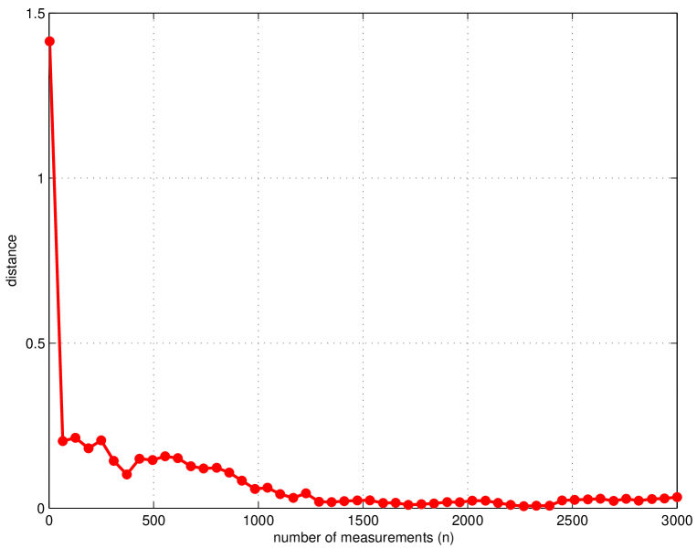
Figure 1: The Hilbert-Schmidt distance between the true pure state (4) and $\Phi_{n}^{{\rm un}}$ does not converge to 0 as $n\to\infty$.

The properties of the unconstrained estimate $\Phi_{n}^{{\rm un}}$ depend very much on the true state. If the eigenvalues of the true state are strictly positive (and not very small), then the estimate is rather good and the convergence is visible from the simulations, see Figure 2 and 3. The simulations are essentially simpler in the $2\times 2$ case, when the boundary of the state space consists of pure states and the positivity of the estimate can be seen from the length of the Bloch vector. In the $3\times 3$ case the boundary is more complicated, it consists of the non-invertible densities.

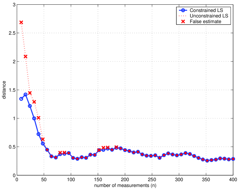
Figure 2: The Hilbert-Schmidt distance between the true $3\times 3$ state with eigenvalues $0.1186,\,0.2871,\,0.5943$ and the estimate. When the number of the measurement is more than 200, the unconstrained estimate gives really a positive semidefinite matrix.

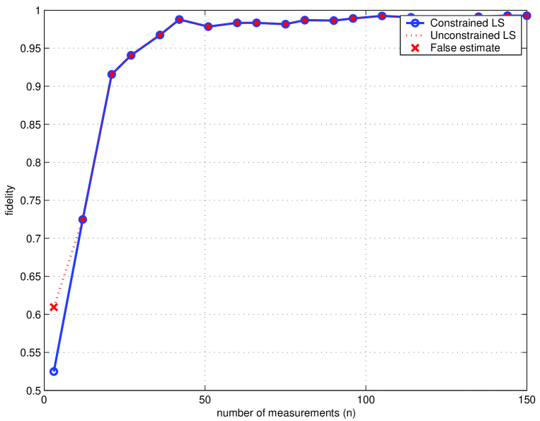
Figure 3: The fidelity between the true $2\times 2$ mixed state and the estimate. When the number of the measurement is more than 10, the unconstrained and the constrained estimates are the same.

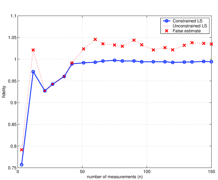
Figure 4: The fidelity between the true $2\times 2$ pure state and the estimates. The unconstrained estimate is often outside of the Bloch ball and in this case the (real part of the complex) fidelity can be bigger than 1. The constrained estimate converges to the true state.

3 Constrained estimate

There are cases when $\Phi_{n}^{{\rm un}}$ is not a positive semidefinite matrix, sometimes we call $\Phi_{n}^{{\rm un}}$ unconstrained estimate. The expectation value of $\Phi_{n}^{{\rm un}}$ is the true state of the system, so it is an unbiased estimate.

We can use the method of least squares to get a density matrix:

$$\Phi_{n}:={\rm argmin}_{\omega}\mbox{Tr}\,(\Phi_{n}^{{\rm un}}-\omega)^{2}={\rm argmin}_{\omega}\sum_{i,j}(\Phi_{n}^{{\rm un}})_{ij}-\omega_{ij})^{2}\,,$$ (5)

where $\omega$ runs over the density matrices. The density matrices form a closed convex set ${\cal D}_{k}$, therefore the minimizer is unique. Note that for a qubit the closest positive semidefinite matrix is easy to find. If the values of the estimates are simply the Bloch vectors, then

$$\Phi_{n}(x)=\cases{\Phi_{n}^{{\rm un}}(x)&if $\|\Phi_{n}^{{\rm un}}(x)\|\leq 1$,\cr\phantom{mm}\cr\displaystyle{\frac{\Phi_{n}^{{\rm un}}(x)}{\|\Phi_{n}^{{\rm un}}(x)\|}}\qquad&otherwise.}$$ (6)

Theorem 2

The constrained estimate $\Phi_{n}$ is asymptotically unbiased.

Proof. We can use the fact that $\Phi_{n}^{{\rm un}}$ is unbiased and to show that $\Phi_{n}$ is an asymptotically unbiased estimate we study their difference. Let $p(x)$ be the probability of the measurement result $x$ and $X$ is the set of outcomes such that $\Phi_{n}^{{\rm un}}(x)\neq\Phi_{n}(x)$, then evidently

$$\sum_{x}\Phi_{n}^{{\rm un}}(x)p(x)-\sum_{x}\Phi_{n}(x)p(x)=\sum_{x\in X}(\Phi_{n}^{{\rm un}}(x)-\Phi_{n}(x))p(x)\,.$$ (7)

If ${\cal D}_{k}\subset{\cal M}_{k}$ is the set of density matrices, then $X$ is the set of outcomes $x$ such that $\Phi_{n}^{{\rm un}}(x)\notin{\cal D}_{k}$. Let us fix a norm on the space ${\cal M}_{k}$. (Note that all norms are equivalent.)

Let $\varepsilon>0$ be arbitrary. We split $X$ into two subsets:

$$X_{1}=\{x\in X:{\rm distance}(\Phi_{n}^{{\rm un}}(x),{\cal D}_{k})\leq\varepsilon\}\quad\mbox{and}\quad X_{2}=X\setminus X_{1}.$$

Note that ${\rm distance}(\Phi_{n}^{{\rm un}}(x),{\cal D}_{k})=\|\Phi_{n}^{{\rm un}}(x)-\Phi_{n}(x)\|$. Then

$$\sum_{x\in X}\|\tilde{\Phi}_{n}(x)-\Phi_{n}(x)\|p(x)\leq\sum_{x\in X_{1}}\|\tilde{\Phi}_{n}(x)-\Phi_{n}(x)\|p(x)+\sum_{x\in X_{2}}\|\tilde{\Phi}_{n}(x)-\Phi_{n}(x)\|p(x)\,.$$

The first term is majorized by $\varepsilon$ and the second one by $C\mbox{Prob}(X_{1})$. Since the first is arbitrary small and the latter goes to $0$, we can conclude that (7) goes to $0$. $\square$

Computing the constrained estimate. The computation of the minimizer of (5) is easier if $\Phi_{n}^{{\rm un}}$ is diagonal, assume that $\Phi_{n}^{{\rm un}}=\mbox{Diag}(x_{1},x_{2},\dots,x_{n})$ and $x_{1},x_{2},\dots,x_{k}<0$ and $x_{k+1},x_{k+2},\dots,x_{n}\geq 0$. The minimizer is obviously diagonal, hence we need to solve

$${\rm argmin}_{y_{i}}\sum_{i}(x_{i}-y_{i})^{2}$$

under the constraint $y_{i}\geq 0$ and $\sum_{i}y_{i}=1$. According to the inequality between the quadratic and arithmetic means, we have

$$\sum_{i=1}^{n}(x_{i}-y_{i})^{2} \geq \sum_{i=1}^{k}x_{i}^{2}+\sum_{i=k+1}^{n}(x_{i}-y_{i})^{2}\geq\sum_{i=1}^{k}x_{i}^{2}+\frac{1}{n-k}\left(\sum_{i=k+1}^{n}(x_{i}-y_{i})\right)^{2}$$

$$= \sum_{i=1}^{k}x_{i}^{2}+\frac{1}{n-k}\left(\sum_{i=1}^{k}y_{i}-x_{i}\right)^{2}.$$

If

$$y_{i}=x_{i}+c\quad\left(i=k+1,k+2,\dots,n,\quad c=\frac{1}{n-k}\sum_{i=1}^{k}x_{i}\right)$$

are positive, then the minimizer is $(y_{1},y_{2},\dots,y_{n})$, where $y_{1}=y_{2}=\dots=y_{k}=0$ and the other $y_{i}$’s are defined above. If the $n$-tuple $(y_{1},y_{2},\dots,y_{n})$ contains negative entries, then we repeat the procedure, the negative entries are replaced with 0 and the actual value of $c$ is added to the other entries. After finitely many steps we arrive at the minimizer. Figure 5 shows the details for $n=3$.

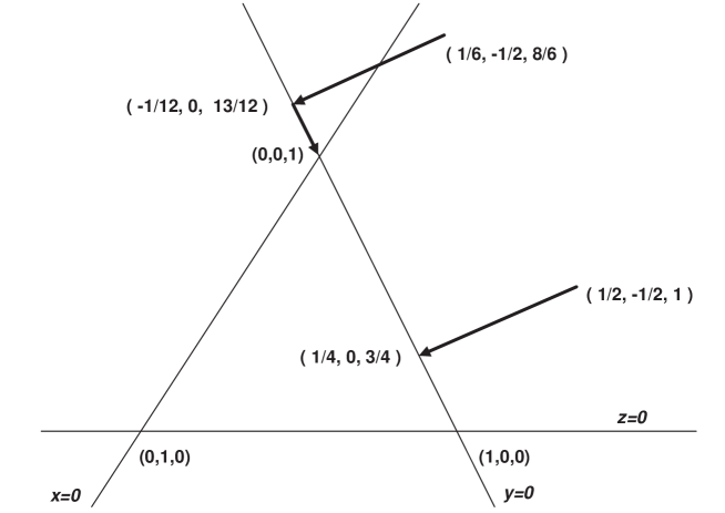
Figure 5: The constrained estimate for $3\times 3$ matrices. The plain $x+y+z=1$ of ${\mathbb{R}}^{3}$ is shown. The triangle $\{(x,y,z):x,y,z\geq 0\}$ corresponds to the diagonal density matrices. Starting from the unconstrained estimate $\mbox{Diag}(1/2,-1/2,1)$, the constrained $\mbox{Diag}(1/4,0,3/4)$ is reached in one step. Starting from $\mbox{Diag}(1/6,-1/2,8/6)$, two steps are needed.

In the general case, we can change the basis such that $\Phi_{n}^{{\rm un}}$ becomes diagonal, since the Hilbert-Schmidt distance is invariant under this transformation. So let $U\Phi_{n}^{{\rm un}}U^{*}=\mbox{Diag}(x_{1},x_{2},\dots,x_{n})$ for a unitary $U$. Then we compute the minimizer $\mbox{Diag}(y_{1},y_{2},\dots,y_{n})$ using the above procedure and

$$\Phi_{n}=U^{*}\mbox{Diag}(y_{1},y_{2},\dots,y_{n})U\,.$$

4 Estimations for a qubit

The mean quadratic error matrix may be used to measure the efficiency of an estimate. If the unknown state is parametrized by $(\theta_{1},\theta_{2},\dots,\theta_{m})$, then the mean quadratic error is an $n\times n$ matrix defined as

$$V_{n}(\theta)_{i,j}:=\sum_{x\in{\cal X}_{n}}(\Phi_{n}(x)_{i}-\theta_{i})(\Phi_{n}(x)_{j}-\theta_{j})\,p(x)\qquad(1\leq i,j\leq n).$$

In case of a qubit, the Bloch parametrization can be used. Then $\theta=(\theta_{1},\theta_{2},\theta_{3})^{t}$ belongs to the unit ball of ${\mathbb{R}}^{3}$. ($(\theta_{1},\theta_{2},\theta_{3})^{t}$ means a column vector, so ^t may be regarded as the transpose.)

Example 2

Assume that the observables

$$A(i)={\mathbb{u}}(i)\cdot\sigma\qquad(1\leq i\leq 3)$$

are measured in the true state

$$\rho_{\theta}=\frac{1}{2}(I+\theta\cdot\sigma)=\frac{1}{2}\left[\begin{array}[]{cc}1+\theta_{3}&\theta_{1}-{\rm i}\theta_{2}\\ \theta_{1}+{\rm i}\theta_{2}&1-\theta_{3}\end{array}\right],$$ (8)

where ${\mathbb{u}}(1),{\mathbb{u}}(2)$ and ${\mathbb{u}}(3)$ are unit vectors in ${\mathbb{R}}^{3}$. The spectral decomposition of $A(i)$ is

$$1\cdot\frac{1}{2}(I+{\mathbb{u}}(i)\cdot\sigma)+(-1)\cdot\frac{1}{2}(I-{\mathbb{u}}(i)\cdot\sigma)$$

and

$$p_{i}:=\mbox{Prob}(A(i)=1)=\frac{1+{\mathbb{u}}(i)\cdot\theta}{2}\,.$$

If the measurements are performed $r$ times, then $\mbox{Prob}(A(i)=1)$ is estimated by the relative frequency $\nu(i)_{r}$ of the outcome $1$. The equations

$$\nu(i)_{r}=\frac{1+{\mathbb{u}}(i)\cdot\hat{\theta}}{2}\qquad(1\leq i\leq 3)$$

should be solved to find an estimate. The solution is

$$\hat{\theta}=T^{-1}(\nu(1)_{r},\nu(2)_{r},\nu(3)_{r})^{t}\,$$ (9)

where ^t denotes the transpose (of a row vector) and the matrix $T$ is

$$T=\left[\begin{array}[]{ccc}{\mathbb{u}}(1)_{1}&{\mathbb{u}}(1)_{2}&{\mathbb{u}}(1)_{3}\\ {\mathbb{u}}(2)_{1}&{\mathbb{u}}(2)_{2}&{\mathbb{u}}(2)_{3}\\ {\mathbb{u}}(3)_{1}&{\mathbb{u}}(3)_{2}&{\mathbb{u}}(3)_{3}\end{array}\right].$$

In particular, if each of the three measurements is performed once and the result is $\varepsilon=(\varepsilon_{1},\varepsilon_{2},\varepsilon_{3})^{t}$, then the unconstrained estimate is

$$\Phi^{{\rm un}}(\varepsilon)=T^{-1}\varepsilon.$$

Similarly to (9), we have

$$\theta=T^{-1}p\,.$$ (10)

The mean quadratic error matrix is the expectation of

$$(T^{-1}\varepsilon-\theta)(T^{-1}\varepsilon-\theta)^{t}=T^{-1}\left((\varepsilon-p)(\varepsilon-p)^{t}\right)(T^{-1})^{*}$$

and the computation yields

$$V^{(1)}(\theta)=T^{-1}\left[\begin{array}[]{ccc}1-({\mathbb{u}}(1)\cdot\theta)^{2}&0&0\\ 0&1-({\mathbb{u}}(2)\cdot\theta)^{2}&0\\ 0&0&1-({\mathbb{u}}(3)\cdot\theta)^{2}\end{array}\right](T^{-1})^{*}.$$ (11)

When each measurement is performed $r$ times, then

$$V_{n}^{(1)}(\theta)=\frac{1}{r}V^{(1)}(\theta),$$

where $n=3r$. If the observables $\sigma_{1},\sigma_{2}$ and $\sigma_{3}$ are measured, then

$$V_{n}^{comp}(\theta)=\frac{1}{r}\left[\begin{array}[]{ccc}1-\theta_{1}^{2}&0&0\\ 0&1-\theta_{2}^{2}&0\\ 0&0&1-\theta_{3}^{2}\end{array}\right].$$ (12)

$\square$

Theorem 3

In the context of the previous example, the determinant of the average mean quadratic error matrix is the smallest, if the vectors ${\mathbb{u}}(1),{\mathbb{u}}(2)$ and ${\mathbb{u}}(3)$ are orthogonal, that is, the observables $A(1),A(2)$ and $A(3)$ are complementary.

Proof. On the parameter space, Bloch ball, we consider the normalized Lebesgue measure. (Any rotationally invariant measure may be considered and gives similar result.) Since

$$\int V_{n}^{(1)}(\theta)\,d\theta = T^{-1}\Big{(}I-\int\mbox{Diag}(({\mathbb{u}}(1)\cdot\theta)^{2},({\mathbb{u}}(2)\cdot\theta)^{2},({\mathbb{u}}(2)\cdot\theta)^{2})d\theta\Big{)}(T^{-1})^{*}$$

$$= C\,(T^{*}T)^{-1}$$

with some positive constant $C$, the determinant is minimal if $\mbox{Det}(T^{*}T)=(\mbox{Det}T)^{2}$ is maximal. $\mbox{Det}\,T$ is the volume of the parallelepipedone determined by the three vectors ${\mathbb{u}}(1),{\mathbb{u}}(2)$ and ${\mathbb{u}}(3)$, and it is maximal when they are orthogonal. $\square$

The content of the theorem is similar to the result of [12], however in the approach of Wootters and Field not the mean quadratic error was minimized but the information gain was maximized. The complementary (or unbiased) measurements are optimal from both view point.

Example 3

Let $\sigma_{i}=P_{i}-Q_{i}$ be the spectral decomposition and let

$$F_{i}=\frac{P_{i}}{3}\quad\mbox{and}\quad F_{i+3}=\frac{Q_{i}}{3}\qquad(1\leq i\leq 3).$$

be a POVM. The corresponding measurement is sometimes called standard qubit tomography [10] and it has 6 outcomes with probabilities

$$p_{i}=\frac{1+\theta_{i}}{6},\quad p_{i+3}=\frac{1-\theta_{i}}{6}\qquad(1\leq i\leq 3).$$

The appropriate (unconstrained) state estimate

$$\Phi(i)=\frac{1}{2}(I+3\sigma_{i})=-I+3P_{i},\quad\Phi(i+3)=\frac{1}{2}(I-3\sigma_{i})=-I+3Q_{i}\,.$$

is unbiased $(1\leq i\leq 3)$. If the true state is $\rho_{\theta}$ of (8), then

$$\sum_{j=1}^{6}p_{j}\Phi(j)=\rho_{\theta}\,.$$

The quadratic error matrix for $n$ independent measurements is

$$V_{n}^{stand}(\theta)=\frac{1}{n}\left[\begin{array}[]{ccc}3-\theta_{1}^{2}&-\theta_{1}\theta_{2}&-\theta_{1}\theta_{3}\\ -\theta_{1}\theta_{2}&3-\theta_{2}^{2}&-\theta_{2}\theta_{3}\\ -\theta_{1}\theta_{3}&-\theta_{2}\theta_{3}&3-\theta_{3}^{2}\end{array}\right].$$ (13)

Proposition 1

In the context of the previous example, the complementary measurement is more efficient than the standard one, i.e. its mean quadratic error matrix is smaller.

Proof. To compare the efficiency of the standard measurement and the complementary measurement, we study the mean quadratic error matrices (12) and (13). The difference $V_{n}^{stand}(\theta)-V_{n}(\theta)$ has the form

$$\frac{1}{n}\left[\begin{array}[]{ccc}3-\theta_{1}^{2}&-\theta_{1}\theta_{2}&-\theta_{1}\theta_{3}\\ -\theta_{1}\theta_{2}&3-\theta_{2}^{2}&-\theta_{2}\theta_{3}\\ -\theta_{1}\theta_{3}&-\theta_{2}\theta_{3}&3-\theta_{3}^{2}\end{array}\right]-\frac{3}{n}\left[\begin{array}[]{ccc}1-\theta_{1}^{2}&0&0\\ 0&1-\theta_{2}^{2}&0\\ 0&0&1-\theta_{3}^{2}\end{array}\right]$$

$$=\frac{1}{n}\left[\begin{array}[]{ccc}2\theta_{1}^{2}&-\theta_{1}\theta_{2}&-\theta_{1}\theta_{3}\\ -\theta_{1}\theta_{2}&2\theta_{2}^{2}&-\theta_{2}\theta_{3}\\ -\theta_{1}\theta_{3}&-\theta_{2}\theta_{3}&2\theta_{3}^{2}\end{array}\right]=\frac{1}{n}\,\left[\begin{array}[]{ccc}2&-1&-1\\ -1&2&-1\\ -1&-1&2\end{array}\right]\circ\left(\left[\begin{array}[]{c}\theta_{1}\\ \theta_{2}\\ \theta_{3}\end{array}\right]\cdot\left[\begin{array}[]{ccc}\theta_{1}&\theta_{2}&\theta_{3}\end{array}\right]\right)$$

where $\circ$ stands for the Hadamard product. Since the Hadamard product of two positive semidefinite matrices is positive semidefinite, we have $V_{n}^{stand}(\theta)\geq V_{n}^{comp}(\theta)$. The complementary measurement is more effective, than the standard one. $\square$

Example 4

Consider the following Bloch vectors

$$a_{1}=\frac{1}{\sqrt{3}}(1,1,1),\qquad\,\,a_{2}=\frac{1}{\sqrt{3}}(1,-1,-1),$$

$$a_{3}=\frac{1}{\sqrt{3}}(-1,1,-1),\quad a_{4}=\frac{1}{\sqrt{3}}(-1,-1,1).$$

and form the positive operators

$$F_{i}=\frac{1}{4}(\sigma_{0}+a_{i}\cdot\sigma)\qquad(1\leq i\leq 4).$$ (16)

They determine a measurement, $\sum_{i=1}^{4}F_{i}=I$. The probability of the outcome $i$ is

$$p_{i}=\mbox{Tr}\,F_{i}\rho_{\theta}=\frac{1}{4}(1+a_{i}\cdot\theta).$$

The above POVM is called minimal qubit tomography by Rehácek, Englert and Kaszlikowski [10].

The matrix-valued estimator

$$\Phi^{min}(i)=-\sigma_{0}+6F_{i}\qquad(1\leq i\leq 4).$$

is unbiased. If the measurement is performed $n$ times, then the average (written in vector-valued form) is

$$\Phi_{n}^{min}=3\sum_{i=1}^{4}\frac{n_{i}}{n}a_{i}\,$$ (17)

where $n_{i}$ is the number of the outcome $i$ from the $n$ measurements. The mean quadratic error matrix is

$$V_{n}^{min}(\theta)=\frac{1}{n}\left[\begin{array}[]{ccc}3-\theta_{1}^{2}&\sqrt{3}\theta_{3}-\theta_{1}\theta_{2}&\sqrt{3}\theta_{2}-\theta_{1}\theta_{3}\\ \sqrt{3}\theta_{3}-\theta_{1}\theta_{2}&3-\theta_{2}^{2}&\sqrt{3}\theta_{1}-\theta_{2}\theta_{3}\\ \sqrt{3}\theta_{2}-\theta_{1}\theta_{3}&\sqrt{3}\theta_{1}-\theta_{2}\theta_{3}&3-\theta_{3}^{2}\end{array}\right].$$ (18)

Unfortunately, the above matrix is not comparable with the mean quadratic error matrix (12), i.e. their difference is indefinite. However, $\mbox{Tr}\,V_{n}^{comp}\leq\mbox{Tr}\,V_{n}^{min}$.

$\square$

5 Conclusion

The estimation of the density matrix of a $k$-level quantum system is studied in this paper. The essential ingredients of an estimation scheme are identified. Those are the parametrization of the density operator $\rho$, the observables to be measured, and the estimator mapping the measured values to an estimate of the density operator. The considered parametrization is given by the real and imaginary part of the entries, and they are estimated by independent measurements. A special set of commuting observables is defined in order to obtain measured values that are classical random variables.

The unconstrained estimate gives a matrix which may be not positive definite and the constrained estimate is the closest density matrix with respect to the Hilbert-Schmidt distance. The constrained estimate is given by a simple procedure starting with the diagonalization of the unconstrained one.

It is established that the properties of the estimation procedure depend very much on the invertibility of the true state. In case of an invertible true state, the unconstrained estimate becomes proper relatively fast. It has been found that for pure states the unconstrained estimates, that are self-adjoint by construction, may not be positive semidefinite and this requires to apply a regularization called constrained estimation procedure.

The estimation procedures carried out by different estimators are compared based on the biasedness of the estimates and their mean quadratic error matrices. In particular, several estimation schemes are compared for the unknown state of a qubit when a single qubit is measured at a time, and its density matrix is parametrized using the Bloch vector. It is shown that the average mean quadratic error matrix is the smallest if the applied observables are complementary.

The results are illustrated by computer simulations.

References

[1]
E. Bagan, M.A. Ballester, R.D. Gill, A. Monras and R. Munoz-Tapia,
Optimal full estimation of qubit mixed states,
Phys. Rev. A 73, 032301, 2006.
[2]
J. A. Bergou, U. Herzog and M. Hillery, Discrimination of quantum states,
in Quantum State Estimation, eds. M. Paris and
J. Rehácek, Lect. Notes Phys. 649, 417-465, 2004.
[3]
G. M. D’Ariano, M. G. A. Paris, and M. F. Sacchi, Quantum tomographic
methods, in Quantum State Estimation, eds. M. Paris and
J. Rehácek, Lect. Notes Phys. 649, 7-58, 2004.
[4]
R. Ellis, Entropy, large deviations, and statistical mechanics,
Springer-Verlag, New York, 1985.
[5]
R. Gill and S. Massar, State estimation for large ensembles,
Phys.Rev. A61, 042312, 2002.
[6]
M. Keyl and R.F. Werner, Estimating the spectrum of a density operator,
Phys. Rev. A 64, 052311, 2001.
[7]
A. Magyar, K.M. Hangos and D. Petz, Computing point estimation
of states of finite quantum systems.
Technical report of the Systems and Control Laboratory
SCL-004/2006, Budapest, http://daedalus.scl.sztaki.hu/
[8]
D. Petz, Complementarity in quantum systems, in preparation.
[9]
D. Petz, K.M. Hangos, A. Szántó and F. Szöllősi,
State tomography for two qubits using reduced densities,
J. Phys. A: Math. Gen. 39, 10901–10907, 2006.
[10]
J. Rehácek, B. Englert and D. Kaszlikowski, Minimal qubit tomography,
Physical Review A 70, 052321, 2004.
[11]
K.G.H. Vollbrecht and R.F. Werner, Why two qubits are special, J. Math. Phys.
41 6772–6782, 2000.
[12]
W.K. Wootters and B.D. Fields, Optimal state determination by mutually
unbiased measurements, Annals of Physics, 191, 363–381, 1989.