Interaction of a two-level atom with squeezed light

Abstract

We consider a degenerate parametric oscillator whose cavity contains a two-level atom. Applying the Heisenberg and quantum Langevin equations, we calculate in the bad-cavity limit the mean photon number, the quadrature variance, and the power spectrum for the cavity mode in general and for the signal light and fluorescent light in particular. We also obtain the normalized second-order correlation function for the fluorescent light. We find that the presence of the two-level atom leads to a decrease in the degree of squeezing of the signal light. It so turns out that the fluorescent light is in a squeezed state and the power spectrum consists of a single peak only.

I Introduction

A considerable interest has been shown in the analysis of the effects of squeezed light on the quantum properties of the fluorescent light emitted by a two-level atom in a cavity. The power spectrum of the fluorescent light emitted by a two-level atom interacting with a cavity mode driven by coherent light and coupled to a squeezed vacuum reservoir has been studied by several authors 1 ; 2 ; 3 ; 4 ; 5 ; 6 ; 7 . Some of these studies show that the width of the incoherent spectrum in the weak driving light limit decreases as the degree of squeezing increases 4 ; 7 . On the other hand, for a strong driving light, the side peaks of the Mollow spectrum are always broadened while the central peak could be broadened or narrowed depending on the relative phase between the strong driving light and the squeezed vacuum 4 ; 7 . Moreover, Agarwal 8 has considered coherently driven $N$ two-level atoms passing through a squeezed cavity mode in the good-cavity limit. He has found modifications of the Mollow triplet due to the presence of the squeezed light. On the other hand, Jin and Xiao 9 have considered $N$ two-level atoms placed inside a parametric oscillator in the good-cavity limit. They have found that under strong-interaction limit, the presence of the two-level atoms inside the parametric oscillator increases the amount of intracavity squeezing from its maximum value of $50\%$ to a maximum value of $75\%$. In addition, Clemens et al. 10 have investigated the power spectrum of the light emitted by a two-level atom inside a parametric oscillator in the week driving light limit. They have found that the incoherent spectrum consists of a vacuum-Rabi doublet with holes in each side band.

In this paper we consider a degenerate parametric oscillator operating below threshold and whose cavity contains a two-level atom. The interaction of the signal light, produced by the parametric amplifier, with the two-level atom leads to the generation of fluorescent light. Thus the cavity mode in this case consists of the signal light and the fluorescent light emitted by the two-level atom. In this paper we analyze the quantum statistical properties of the fluorescent and the signal light applying the Heisenberg and quantum Langevin equations in the bad-cavity limit. This system can also be studied using the master equation in the bad-cavity limit. Employing the bad-cavity limit, one usually obtains the master equation for the atomic density operator. Hence it will not be possible in this approach to study the properties of the cavity mode. The method used in this paper enables us to study not only the properties of the fluorescent light emitted by the two-level atom but also the properties of the cavity mode.

We derive the equations of evolution for the expectation values of atomic and cavity mode operators using the Heisenberg and quantum Langevin equations in the bad-cavity limit. Applying the resulting equations, we calculate the mean photon number, the quadrature variance, and the power spectrum for the cavity mode, for the signal light, and for the fluorescent light. We also determine the second order correlation function for the fluorescent light.

II Equations of Evolution of atomic expectation values

We consider a single two-level atom inside a parametric oscillator coupled to a vacuum reservoir. We represent the upper and lower levels of the atom by $|a\rangle$ and $|b\rangle$ and we assume the atom to be at resonance with the cavity mode (see Fig. 1). In a degenerate parametric oscillator, a pump photon of frequency $2\omega$ is down converted into a pair of highly correlated signal photons each of frequency $\omega$. It so turns out that the signal light is in a squeezed state. Contrary to the work of Clemens et al. 10 where they considered weak squeezed light (two photons in the cavity at a time), we have not imposed any restriction on the number of signal photons in the cavity. With the pump mode treated classically, the parametric interaction can be described by the Hamiltonian  11

Figure 1: A single two-level atom inside a parametric oscillator.

$$\hat{H}_{1}=\frac{i\varepsilon}{2}(\hat{a}^{\dagger 2}-\hat{a}^{2}),$$ (1)

in which $\varepsilon$, assumed to be real and constant, is proportional to the amplitude of the pump mode and $\hat{a}$ is the annihilation operator for the cavity mode. In addition, the interaction of the cavity mode with the two-level atom is describable by the Hamiltonian

$$\hat{H}_{2}=ig(\hat{\sigma}_{+}\hat{a}-\hat{a}^{\dagger}\sigma_{-}),$$ (2)

where $g$ is the atom-cavity mode coupling constant and $\hat{\sigma}_{\pm}$ are atomic operators satisfying the commutation relations $[\hat{\sigma}_{+},\hat{\sigma}_{-}]=\hat{\sigma}_{z}$ and $[\hat{\sigma}_{\pm},\hat{\sigma}_{z}]=\mp 2\hat{\sigma}_{\pm}$. Thus the Hamiltonian describing the parametric interaction and the interaction of the cavity mode with the two-level has the form

$$H={i\varepsilon\over 2}(\hat{a}^{\dagger 2}-\hat{a}^{2})+ig(\hat{\sigma}_{+}\hat{a}-\hat{a}^{\dagger}\sigma_{-}).$$ (3)

Applying the Heisenberg equation, one can readily establish that the time evolution of the atomic operators are of the form

$$\frac{d}{dt}\hat{\sigma}_{-}=-g\hat{\sigma}_{z}\hat{a},$$ (4)

$$\frac{d}{dt}\hat{\sigma}_{z}=2g\hat{a}^{\dagger}\hat{\sigma}_{-}+2g\hat{\sigma}_{+}\hat{a}.$$ (5)

On the other hand, the quantum Langevin equation for the cavity mode operator $\hat{a}$ is expressible as

$$\frac{d}{dt}\hat{a}=-i[\hat{a},\hat{H}]-\frac{\kappa}{2}\hat{a}+\hat{F},$$ (6a)

so that on account of Eq. (3), there follows

$$\frac{d}{dt}\hat{a}=-\frac{\kappa}{2}\hat{a}+\varepsilon\hat{a}^{\dagger}-g\hat{\sigma}_{-}+\hat{F},$$ (6b)

where $\kappa$ is the cavity damping constant and $\hat{F}$ is a noise operator associated with the vacuum reservoir and having the following correlation properties:

$$\langle\hat{F}(t)\rangle=0,$$ (7a)

$$\langle\hat{F}^{\dagger}(t)\hat{F}(t^{\prime})\rangle=0,$$ (7b)

$$\langle\hat{F}(t)\hat{F}^{\dagger}(t^{\prime})\rangle=\kappa\delta(t-t^{\prime}),$$ (7c)

$$\langle\hat{F}^{\dagger}(t)\hat{F}^{\dagger}(t^{\prime})\rangle=\langle\hat{F}(t)\hat{F}(t^{\prime})\rangle=0.$$ (7d)

Since Eqs. (4), (5), and (6b) are nonlinear and coupled differential equations, it is not possible to obtain exact solutions. We then seek to obtain the solutions of these equations applying the bad-cavity limit. In the bad-cavity limit, the cavity damping constant is much greater than the cavity atomic decay rate. In this limit, the cavity mode variables decay faster than the atomic variables. We can then set the time derivatives of the cavity mode variables equal to zero while keeping the zero-order atomic and cavity mode variables at time t. In view of this, we obtain from Eq. (6b) that

$$\hat{a}(t)= -\frac{2\kappa g}{\kappa^{2}-4\varepsilon^{2}}\hat{\sigma}_{-}(t)-\frac{4g\varepsilon}{\kappa^{2}-4\varepsilon^{2}}\hat{\sigma}_{+}(t)$$

$$+\frac{4}{\kappa^{2}-4\varepsilon^{2}}(\frac{\kappa}{2}\hat{F}(t)+\varepsilon\hat{F}^{\dagger}(t)).$$ (8)

This result will be used to calculate the expectation values of the products of a cavity mode operator and an atomic operator. Then introduction of Eq. (II) into (4) and (5) leads to

$$\frac{d}{dt}\hat{\sigma}_{-} =-\frac{2g^{2}/\kappa}{1-4\varepsilon^{2}/\kappa^{2}}\hat{\sigma}_{-}+\frac{4g^{2}\varepsilon/\kappa^{2}}{1-4\varepsilon^{2}/\kappa^{2}}\hat{\sigma}_{+}$$

$$-\frac{4g}{\kappa^{2}-4\varepsilon^{2}}\big{[}\frac{\kappa}{2}\hat{\sigma}_{z}\hat{F}+\varepsilon\hat{\sigma}_{z}\hat{F}^{\dagger}\big{]},$$ (9)

$$\frac{d}{dt}\hat{\sigma}_{z} =-\frac{8g^{2}/\kappa}{1-4\varepsilon^{2}/\kappa^{2}}\hat{\sigma}_{+}\hat{\sigma}_{-}$$

$$+\frac{8g}{\kappa^{2}-4\varepsilon^{2}}\big{[}\frac{\kappa}{2}(\hat{F}^{\dagger}\hat{\sigma}_{-}+\hat{\sigma}_{+}\hat{F})+\varepsilon(\hat{F}\hat{\sigma}_{-}+\hat{\sigma}_{+}\hat{F}^{\dagger})\big{]},$$ (10)

or

$$\frac{d}{dt}\langle\hat{\sigma}_{-}\rangle =-\frac{2g^{2}/\kappa}{1-4\varepsilon^{2}/\kappa^{2}}\langle\hat{\sigma}_{-}\rangle+\frac{4g^{2}\varepsilon/\kappa^{2}}{1-4\varepsilon^{2}/\kappa^{2}}\langle\hat{\sigma}_{+}\rangle$$

$$-\frac{4g}{\kappa^{2}-4\varepsilon^{2}}\big{[}\frac{\kappa}{2}\langle\hat{\sigma}_{z}\hat{F}\rangle+\varepsilon\langle\hat{\sigma}_{z}\hat{F}^{\dagger}\rangle\big{]},$$ (11)

$$\frac{d}{dt}\langle\hat{\sigma}_{z}\rangle=-\frac{8g^{2}/\kappa}{1-4\varepsilon^{2}/\kappa^{2}}\langle\hat{\sigma}_{+}\hat{\sigma}_{-}\rangle$$

$$+\frac{8g}{\kappa^{2}-4\varepsilon^{2}}\big{[}\frac{\kappa}{2}(\langle\hat{F}^{\dagger}\hat{\sigma}_{-}\rangle+\langle\hat{\sigma}_{+}\hat{F}\rangle)+\varepsilon(\langle\hat{F}\hat{\sigma}_{-}\rangle+\langle\hat{\sigma}_{+}\hat{F}^{\dagger}\rangle)\big{]}.$$ (12)

We note that Eq. (II) has a well-behaved solution provided that $\eta=(4g^{2}/\kappa)/(1-4\varepsilon^{2}/\kappa^{2})$ is positive. This will be the case if $\varepsilon/\kappa<1/2$.

We next proceed to find the expectation values of the products involving a noise operator and an atomic operator that appear in Eqs. (II) and (II). To this end, the formal solution of Eq. (II) can be written as

$$\hat{\sigma}_{-}(t) =\hat{\sigma}_{-}(0)e^{-\eta t/2}$$

$$+\int_{0}^{t}e^{-\eta(t-t^{\prime})/2}\big{[}\eta(\varepsilon/\kappa)\hat{\sigma}_{+}(t^{\prime})-\frac{4g}{\kappa^{2}-4\varepsilon^{2}}$$

$$\times\big{(}\frac{\kappa}{2}\hat{\sigma}_{z}(t^{\prime})\hat{F}(t^{\prime})+\varepsilon\hat{\sigma}_{z}(t^{\prime})\hat{F}^{\dagger}(t^{\prime})\big{)}\big{]}dt^{\prime},$$ (13)

so that multiplying this equation on the left by $\hat{F}(t)$ and taking the expectation value of the resulting expression, we obtain

$$\langle\hat{F}(t)\hat{\sigma}_{-}(t)\rangle=\langle\hat{F}(t)\hat{\sigma}_{-}(0)\rangle e^{-\eta t/2}$$

$$+\int_{0}^{t}e^{-\eta(t-t^{\prime})/2}\big{[}\eta(\varepsilon/\kappa)\langle\hat{F}(t)\hat{\sigma}_{+}(t^{\prime})\rangle-\frac{4g}{\kappa^{2}-4\varepsilon^{2}}$$

$$\times\big{(}\frac{\kappa}{2}\langle\hat{F}(t)\hat{\sigma}_{z}(t^{\prime})\hat{F}(t^{\prime})\rangle+\varepsilon\langle\hat{F}(t)\hat{\sigma}_{z}(t^{\prime})\hat{F}^{\dagger}(t^{\prime})\rangle\big{)}\big{]}dt^{\prime}.$$ (14)

It is not possible to evaluate the integral that appears in Eq. (II) as the explicit form of $\hat{\sigma}_{z}(t^{\prime})$ is unknown yet. In order to proceed further, we need to adopt a certain approximation scheme. To this end, ignoring the noncommutativity of the atomic and noise operators, we see that $\langle\hat{F}(t)\hat{\sigma}_{z}(t^{\prime})\hat{F}(t^{\prime})\rangle=\langle\hat{\sigma}_{z}(t^{\prime})\hat{F}(t)\hat{F}(t^{\prime})\rangle$. Then upon neglecting the correlation between $\hat{\sigma}_{z}(t^{\prime})$ and $\hat{F}(t)\hat{F}(t^{\prime})$, assumed to be considerably small, one can write the approximately valid relation 12 $\langle\hat{F}(t)\hat{\sigma}_{z}(t^{\prime})\hat{F}(t^{\prime})\rangle=\langle\hat{\sigma}_{z}(t^{\prime})\hat{F}(t)\hat{F}(t^{\prime})\rangle=\langle\hat{\sigma}_{z}(t^{\prime})\rangle\langle\hat{F}(t)\hat{F}(t^{\prime})\rangle$. Following a similar line of reasoning, one can also write the approximately valid relation $\langle\hat{F}(t)\hat{\sigma}_{z}(t^{\prime})\hat{F}^{\dagger}(t^{\prime})\rangle=\langle\hat{\sigma}_{z}(t^{\prime})\hat{F}(t)\hat{F}^{\dagger}(t^{\prime})\rangle=\langle\hat{\sigma}_{z}(t^{\prime})\rangle\langle\hat{F}(t)\hat{F}^{\dagger}(t^{\prime})\rangle$. Now using these approximations and taking into account the fact that a noise operator $\hat{F}$ at time t does not affect the atomic variables at earlier times, Eq. (II) can be put in the form

$$\langle\hat{F}(t)\hat{\sigma}_{-}(t)\rangle =-\frac{4g}{\kappa^{2}-4\varepsilon^{2}}\int_{0}^{t}e^{-\eta(t-t^{\prime})/2}\langle\hat{\sigma}_{z}(t)^{\prime}\rangle$$

$$\times\big{(}\frac{\kappa}{2}\langle\hat{F}(t)\hat{F}(t^{\prime})\rangle+\varepsilon\langle\hat{F}(t)\hat{F}^{\dagger}(t^{\prime})\rangle\big{)}dt^{\prime}.$$ (15)

Therefore using Eqs. (7c) and (7d) and performing the integration, we find

$$\langle\hat{F}(t)\hat{\sigma}_{-}(t)\rangle=-\frac{(2g\varepsilon/\kappa)\langle\hat{\sigma}_{z}(t)\rangle}{1-4\varepsilon^{2}/\kappa^{2}}.$$ (16)

We immediately notice that

$$\langle\hat{\sigma}_{+}(t)\hat{F}^{\dagger}(t)\rangle=-\frac{(2g\varepsilon/\kappa)\langle\hat{\sigma}_{z}(t)\rangle}{1-4\varepsilon^{2}/\kappa^{2}}.$$ (17)

It can also be readily established in a similar manner that

$$\langle\hat{\sigma}_{+}(t)\hat{F}(t)\rangle=\langle\hat{F}^{\dagger}(t)\hat{\sigma}_{-}(t)\rangle=0,$$ (18a)

$$\langle\hat{\sigma}_{-}(t)\hat{F}(t)\rangle=\langle\hat{F}^{\dagger}(t)\sigma_{+}(t)\rangle=0,$$ (18b)

$$\langle\hat{\sigma}_{-}(t)\hat{F}^{\dagger}(t)\rangle=\langle\hat{F}(t)\hat{\sigma}_{+}(t)\rangle=-\frac{g\langle\hat{\sigma}_{z}(t)\rangle}{1-4\varepsilon^{2}/\kappa^{2}},$$ (19)

$$\langle\hat{\sigma}_{z}(t)\hat{F}(t)\rangle=0,$$ (20)

$$\langle\hat{\sigma}_{z}(t)\hat{F}^{\dagger}(t)\rangle=\frac{4g/\kappa}{1-4\varepsilon^{2}/\kappa^{2}}(\frac{\kappa}{2}\langle\hat{\sigma}_{+}\rangle+\varepsilon\langle\hat{\sigma}_{-}\rangle).$$ (21)

With the aid of Eqs. (16)-(18), (20), (21), and employing the relation $\hat{\sigma}_{+}\hat{\sigma}_{-}=(\hat{\sigma}_{z}+1)/2$, Eqs. (II) and (II) can be written as

$$\frac{d}{dt}\langle\hat{\sigma}_{-}\rangle= -\frac{\Gamma}{2}\langle\hat{\sigma}_{-}\rangle-\frac{\varepsilon}{\kappa}\Gamma\langle\hat{\sigma}_{+}\rangle,$$ (22)

$$\frac{d}{dt}\langle\hat{\sigma}_{z}\rangle=-\Gamma\langle\hat{\sigma}_{z}\rangle-\eta,$$ (23)

where $\Gamma=(4g^{2}/\kappa)(1+4\varepsilon^{2}/\kappa^{2})/(1-4\varepsilon^{2}/\kappa^{2})^{2}$ is the cavity atomic decay rate. In view of the fact that $\langle\hat{\sigma}_{-}(t)\rangle^{*}=\langle\hat{\sigma}_{+}(t)\rangle$ and $\langle\hat{\sigma}_{z}(t)\rangle^{*}=\langle\hat{\sigma}_{z}(t)\rangle$ one can write

$$\frac{d}{dt}\langle\hat{\sigma}_{+}\rangle= -\frac{\Gamma}{2}\langle\hat{\sigma}_{+}\rangle-\frac{\varepsilon}{\kappa}\Gamma\langle\hat{\sigma}_{-}\rangle.$$ (24)

In the absence of the parametric amplifier the cavity atomic decay rate is $\gamma_{c}=4g^{2}/\kappa$. Thus we can express $\Gamma$ as $\Gamma=\gamma_{c}(1+4\varepsilon^{2}/\kappa^{2})/(1-4\varepsilon^{2}/\kappa^{2})^{2}$. It can be easily seen that the presence of the parametric amplifier enhances the cavity atomic decay rate.

III Power spectrum and photon antibunching of the fluorescent light

The power spectrum of the fluorescent light can be expressed as 12

$$S(\omega)=2Re\int_{0}^{\infty}\langle\hat{\sigma}_{+}(t)\hat{\sigma}_{-}(t+\tau)\rangle_{ss}e^{i\omega\tau}d\tau.$$ (25)

Introducing new variables defined by $z_{\pm}=\langle\hat{\sigma}_{-}\rangle\pm\langle\hat{\sigma}_{+}\rangle$ and applying Eqs. (22) and (24), we get

$$\frac{d}{dt}z_{\pm}=-\lambda_{\pm}z_{\pm},$$ (26)

where $\lambda_{\pm}=\Gamma(\frac{1}{2}\pm\frac{\varepsilon}{\kappa})$. The solution of this equation can be written in the form

$$z_{\pm}(t+\tau)=z_{\pm}(t)e^{-\lambda_{\pm}\tau}.$$ (27)

It then follows that

$$\langle\hat{\sigma}_{-}(t+\tau)\rangle =\frac{1}{2}\langle\hat{\sigma}_{-}(t)\rangle(e^{-\lambda_{+}\tau}+e^{-\lambda_{-}\tau})$$

$$+\frac{1}{2}\langle\hat{\sigma}_{+}(t)\rangle(e^{-\lambda_{+}\tau}-e^{-\lambda_{-}\tau}).$$ (28)

Now applying the quantum regression theorem, we have

$$\langle\hat{\sigma}_{+}(t)\hat{\sigma}_{-}(t+\tau)\rangle_{ss}=\frac{1}{2}\langle\hat{\sigma}_{+}(t)\hat{\sigma}_{-}(t)\rangle_{ss}(e^{-\lambda_{+}\tau}+e^{-\lambda_{-}\tau}).$$ (29)

The steady state solution of Eq. (23) is

$$\langle\hat{\sigma}_{z}(t)\rangle_{ss}=\frac{-\eta}{\Gamma},$$ (30)

from which follows

$$(\langle\hat{\sigma}_{z}(t)\rangle_{ss}+1)/2=\frac{\Gamma-\eta}{2\Gamma}.$$ (31)

In view of the relation $\langle\hat{\sigma}_{+}(t)\hat{\sigma}_{-}(t)\rangle_{ss}=(\langle\hat{\sigma}_{z}(t)\rangle_{ss}+1)/2$ and Eq. (31), we see that

$$\langle\hat{\sigma}_{+}(t)\hat{\sigma}_{-}(t)\rangle_{ss}=\frac{\Gamma-\eta}{2\Gamma}$$ (32)

Now upon substituting (32) into (29), we obtain

$$\langle\hat{\sigma}_{+}(t)\hat{\sigma}_{-}(t+\tau)\rangle_{ss}=\frac{\Gamma-\eta}{4\Gamma}(e^{-\lambda_{+}\tau}+e^{-\lambda_{-}\tau}).$$ (33)

On account of this result the power spectrum takes the form

$$S(\omega)=\frac{\Gamma-\eta}{2\Gamma}Re\int_{0}^{\infty}(e^{-(\lambda_{+}-i\omega)\tau}+e^{-(\lambda_{-}-i\omega)\tau})d\tau.$$ (34)

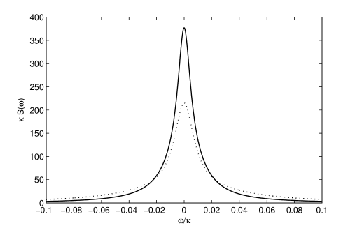
Figure 2: Plots of the power spectrum of the fluorescent light [Eq. (35)] versus $\omega/\kappa$ for $\gamma_{c}/\kappa=0.01$, for $\varepsilon/\kappa=0.25$ (solid curve) and for $\varepsilon/\kappa=0.35$ (dotted curve).

Hence the normalized power spectrum is found to be

$$S(\omega)=\frac{\Gamma(\frac{1}{2}+\frac{\varepsilon}{\kappa})/2\pi}{\Gamma^{2}(\frac{1}{2}+\frac{\varepsilon}{\kappa})^{2}+\omega^{2}}+\frac{\Gamma(\frac{1}{2}-\frac{\varepsilon}{\kappa})/2\pi}{\Gamma^{2}(\frac{1}{2}-\frac{\varepsilon}{\kappa})^{2}+\omega^{2}}.$$ (35)

Expression (35) indicates that the power spectrum of the fluorescent light is the sum of two Lorentzians centered at zero frequency and having half widths of $\Gamma(\frac{1}{2}+\frac{\varepsilon}{\kappa})$ and $\Gamma(\frac{1}{2}-\frac{\varepsilon}{\kappa})$. Fig. 2 shows that the power spectrum of the fluorescent light is a single peak centered at $\omega=0$. We have found that the half width of the power spectrum increases from $0.0070$ to $0.0101$ as $\varepsilon/\kappa$ increases from $0.25$ to $0.35$. Contrary to the power spectrum of the fluorescent light from a two-level atom driven by a strong coherent light 4 ; 7 , the power spectrum in this case turns out to be a single peak.

The second order correlation function can be expressed in terms of the atomic operators as

$$g^{(2)}(\tau)=\frac{\langle\hat{\sigma}_{+}(t)\hat{\sigma}_{+}(t+\tau)\hat{\sigma}_{-}(t+\tau)\hat{\sigma}_{-}(t)\rangle}{\langle\hat{\sigma}_{+}(t)\hat{\sigma}_{-}(t)\rangle^{2}}.$$ (36)

We recall that

$$\langle\hat{\sigma}_{+}(t+\tau)\hat{\sigma}_{-}(t+\tau)\rangle=(\langle\hat{\sigma}_{z}(t+\tau)\rangle+1)/2.$$ (37)

Furthermore, the formal solution of Eq. (23) can be written as

$$\langle\hat{\sigma}_{z}(t+\tau)\rangle=\langle\hat{\sigma}_{z}(t)\rangle e^{-\Gamma\tau}-\frac{\eta}{\Gamma}(1-e^{-\Gamma\tau}),$$ (38)

from which follows

$$(\langle\hat{\sigma}_{z}(t+\tau)\rangle+1)/2 =\frac{1}{2}(\langle\hat{\sigma}_{z}(t)\rangle+1)e^{-\Gamma\tau}$$

$$+\frac{\Gamma-\eta}{2\Gamma}(1-e^{-\Gamma\tau}).$$ (39)

In view of Eq. (37), we see that

$$\langle\hat{\sigma}_{+}(t+\tau)\hat{\sigma}_{-}(t+\tau)\rangle=\langle\hat{\sigma}_{+}(t)\hat{\sigma}_{-}(t)\rangle e^{-\Gamma\tau}+\frac{\Gamma-\eta}{2\Gamma}(1-e^{-\Gamma\tau}).$$ (40)

On applying the quantum regression theorem, the second-order correlation function can be written as

$$g^{(2)}(\tau)=\frac{(\Gamma-\eta)/2\Gamma}{\langle\hat{\sigma}_{+}(t)\hat{\sigma}_{-}(t)\rangle}(1-e^{-\Gamma\tau}).$$ (41)

Thus in view (32), the steady-state second order correlation function becomes

$$g^{(2)}(\tau)=1-e^{-\Gamma\tau}.$$ (42)

We observe that $g^{(2)}(0)=0$ and for $\tau>0$, $g^{(2)}(\tau)>0$. Therefore we see that for $\tau>0$, $g^{(2)}(\tau)>g^{(2)}(0)$. The fluorescent light thus exhibits the phenomenon of photon antibunching, as is always the case. This is due to the fact that a two-level atom cannot emit two or more photons simultaneously. After each emission the atom returns to the lower level and it must absorb a photon before another emission can take place. Fig. 3 indicates that for relatively small values of $\tau$ the second-order correlation function is less than unity which reflects the nonclassical feature of antibunching. We also observe that as $\varepsilon/\kappa$ increases $g^{(2)}(\tau)$ approaches unity at a faster rate.

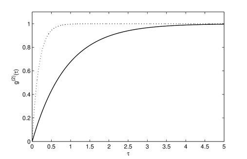
Figure 3: Plots of the second order correlation function [Eq. (42)] versus $\tau$ for $\gamma_{c}/\kappa=0.01$, for $\varepsilon/\kappa=0.10$ (solid curve), for $\varepsilon/\kappa=0.35$ (dotted curve).

It is also interesting to consider the dynamics of the two-level atom. Thus upon replacing $\tau$ by $t$ and $t$ by $0$ in Eq. (III) and using the relation $\langle\hat{\sigma}_{+}(t)\hat{\sigma}_{-}(t)\rangle=(\langle\hat{\sigma}_{z}(t)\rangle+1)/2$, the probability for the two-level atom to be in the upper level is found to be

$$\rho_{aa}(t)=\rho_{aa}(0)e^{-\Gamma t}+\frac{4\varepsilon^{2}/\kappa^{2}}{1+4\varepsilon^{2}/\kappa^{2}}(1-e^{-\Gamma t}).$$ (43)

If the atom is initially in the upper level, then $\rho_{aa}(0)=1$. Hence Eq. (43) takes for this case the form

$$\rho_{aa}(t)=\frac{e^{-\Gamma t}}{1+4\varepsilon^{2}/\kappa^{2}}+\frac{4\varepsilon^{2}/\kappa^{2}}{1+4\varepsilon^{2}/\kappa^{2}}$$ (44)

and at steady state, we have

$$\rho_{aa}=\frac{4\varepsilon^{2}/\kappa^{2}}{1+4\varepsilon^{2}/\kappa^{2}}.$$ (45)

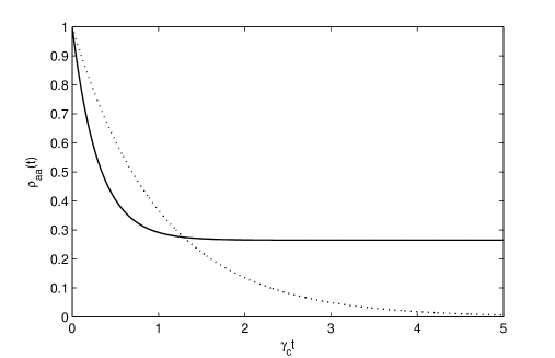
Figure 4: Plots of [Eq. (44)] versus $\gamma_{c}t$ in the presence of the parametric amplifier with $\varepsilon/\kappa=0.3$ (solid curve) and in the absence of the parametric amplifier, i.e, for $\varepsilon=0$ (dotted curve).

We see from Fig. 4 that the probability for the atom to be in the upper level decays exponentially in the absence of the parametric amplifier and approaches to zero at steady state. However, in the presence of the parametric amplifier the steady state probability for the atom to be in the upper level is different from zero. This is because there are photons in the cavity that can be absorbed by the atom.

IV Quadrature variance

In this section we calculate the mean photon number and the quadrature variance for the cavity mode. Moreover, we determine the mean photon number and the quadrature variance for the signal light and for the fluorescent light. The variance of the quadrature operators defined by  11

$$\hat{a}_{+}=\hat{a}^{\dagger}+\hat{a}$$ (46)

and

$$\hat{a}_{-}=i(\hat{a}^{\dagger}-\hat{a}),$$ (47)

can be expressed as

$$\Delta\hat{a}_{\pm}^{2}=1\pm(\langle\hat{a}^{\dagger^{2}}\rangle+\langle\hat{a}^{2}\rangle\pm 2\langle\hat{a}^{\dagger}\hat{a}\rangle)\mp(\langle\hat{a}^{\dagger}\rangle\pm\langle\hat{a}\rangle)^{2}.$$ (48)

On account Eqs. (7a), (II), and (III), we easily see that

$$\langle\hat{a}^{\dagger}\rangle_{ss}=\langle\hat{a}\rangle_{ss}=0.$$ (49)

Thus the quadrature variance takes at steady state the form

$$\Delta\hat{a}_{\pm}^{2}=1+2\langle\hat{a}^{\dagger}\hat{a}\rangle_{ss}\pm(\langle\hat{a}^{\dagger^{2}}\rangle_{ss}+\langle\hat{a}^{2}\rangle_{ss}).$$ (50)

We now proceed to calculate the steady state expectation values of the second-order cavity mode variables. Employing Eq. (6b), one can readily obtain

$$\frac{d}{dt}\langle\hat{a}^{2}\rangle =-\kappa\langle\hat{a}^{2}\rangle+2\varepsilon\langle\hat{a}^{\dagger}\hat{a}\rangle+\varepsilon-g(\langle\hat{a}\hat{\sigma}_{-}\rangle+\langle\hat{\sigma}_{-}\hat{a}\rangle)$$

$$+\langle\hat{a}\hat{F}\rangle+\langle\hat{F}\hat{a}\rangle,$$ (51)

$$\frac{d}{dt}\langle\hat{a}^{\dagger}\hat{a}\rangle =-\kappa\langle\hat{a}^{\dagger}\hat{a}\rangle+\varepsilon(\langle\hat{a}^{2}\rangle+\langle\hat{a}^{\dagger 2}\rangle)$$

$$-g(\langle\hat{a}^{\dagger}\hat{\sigma}_{-}\rangle+\langle\hat{\sigma}_{+}\hat{a}\rangle)+\langle\hat{a}^{\dagger}\hat{F}\rangle+\langle\hat{F}^{\dagger}\hat{a}\rangle.$$ (52)

The formal solution of Eq. (6b) can be expressed as

$$\hat{a}(t)=\hat{a}(0)e^{-\kappa t/2}+\int_{0}^{t}e^{-\kappa(t-t^{\prime})/2}[\varepsilon\hat{a}^{\dagger}(t^{\prime})-g\hat{\sigma}_{-}(t^{\prime})+\hat{F}(t^{\prime})]dt^{\prime},$$ (53)

so that multiplying on the right by $\hat{F}(t)$ and taking the expectation value, we get

$$\langle\hat{a}(t)\hat{F}(t)\rangle =\langle\hat{a}(0)\hat{F}(t)\rangle e^{-\kappa t/2}+\int_{0}^{t}e^{-\kappa(t-t^{\prime})/2}[\varepsilon\langle\hat{a}^{\dagger}(t^{\prime})\hat{F}(t)\rangle$$

$$-g\langle\hat{\sigma}_{-}(t^{\prime})\hat{F}(t)\rangle+\langle\hat{F}(t^{\prime})\hat{F}(t)\rangle]dt^{\prime}.$$ (54)

On account of Eq. (7d) and the fact that the noise operator at time $t$ does not affect the system variables at earlier times, Eq. (IV) reduces to

$$\langle\hat{a}(t)\hat{F}(t)\rangle=0.$$ (55)

It can also be established in a similar manner that

$$\langle\hat{F}(t)\hat{a}(t)\rangle=0.$$ (56)

Furthermore, applying Eq. (II) along with Eqs. (16), (18), and (19), one easily obtains

$$\langle\hat{a}\hat{\sigma}_{-}\rangle=-\frac{4g\varepsilon/\kappa^{2}}{1-4\varepsilon^{2}/\kappa^{2}}\langle\hat{\sigma}_{+}\hat{\sigma}_{-}\rangle-\frac{4g\varepsilon/\kappa^{2}}{(1-4\varepsilon^{2}/\kappa^{2})^{2}}\langle\hat{\sigma}_{z}\rangle$$ (57)

and

$$\langle\hat{\sigma}_{-}\hat{a}\rangle=-\frac{4g\varepsilon/\kappa^{2}}{1-4\varepsilon^{2}/\kappa^{2}}\langle\hat{\sigma}_{-}\hat{\sigma}_{+}\rangle-\frac{4g\varepsilon/\kappa^{2}}{(1-4\varepsilon^{2}/\kappa^{2})^{2}}\langle\hat{\sigma}_{z}\rangle.$$ (58)

Upon substituting Eqs. (55)-(58) into (IV), we find

$$\frac{d}{dt}\langle\hat{a}^{2}\rangle =-\kappa\langle\hat{a}^{2}\rangle+2\varepsilon\langle\hat{a}^{\dagger}\hat{a}\rangle+\varepsilon+\frac{\gamma_{c}\varepsilon/\kappa}{1-4\varepsilon^{2}/\kappa^{2}}$$

$$+\frac{2\gamma_{c}\varepsilon/\kappa}{(1-4\varepsilon^{2}/\kappa^{2})^{2}}\langle\hat{\sigma}_{z}\rangle.$$ (59)

Following a similar procedure, one can put Eq. (IV) in the form

$$\frac{d}{dt}\langle\hat{a}^{\dagger}\hat{a}\rangle =-\kappa\langle\hat{a}^{\dagger}\hat{a}\rangle+\varepsilon(\langle\hat{a}^{\dagger 2}\rangle+\langle\hat{a}^{2}\rangle)$$

$$+\frac{\gamma_{c}}{1-4\varepsilon^{2}/\kappa^{2}}\langle\hat{\sigma}_{+}\hat{\sigma}_{-}\rangle+\frac{4\gamma_{c}\varepsilon^{2}/\kappa^{2}}{(1-4\varepsilon^{2}/\kappa^{2})^{2}}\langle\hat{\sigma}_{z}\rangle.$$ (60)

On account of (30) and (32), Eqs. (IV) and (IV) reduce at steady state to

$$\langle\hat{a}^{2}\rangle_{ss} =\frac{2\varepsilon}{\kappa}\langle\hat{a}^{\dagger}\hat{a}\rangle_{ss}+\frac{\varepsilon}{\kappa}+\frac{\gamma_{c}\varepsilon/\kappa^{2}}{1-4\varepsilon^{2}/\kappa^{2}}$$

$$-\frac{2\gamma_{c}\varepsilon/\kappa^{2}}{(1+4\varepsilon^{2}/\kappa^{2})(1-4\varepsilon^{2}/\kappa^{2})}$$ (61)

and

$$\langle\hat{a}^{\dagger}\hat{a}\rangle_{ss}=\frac{\varepsilon}{\kappa}(\langle\hat{a}^{2}\rangle_{ss}+\langle\hat{a}^{\dagger 2}\rangle_{ss}).$$ (62)

Now with the aid of (IV) and (62), the mean photon number of the cavity mode is found at steady state to be

$$\langle\hat{a}^{\dagger}\hat{a}\rangle_{ss} =\frac{2\varepsilon^{2}/\kappa^{2}}{1-4\varepsilon^{2}/\kappa^{2}}-\frac{4\gamma_{c}\varepsilon^{2}/\kappa^{3}}{(1-4\varepsilon^{2}/\kappa^{2})^{2}(1+4\varepsilon^{2}/\kappa^{2})}$$

$$+\frac{(\gamma_{c}/2\kappa)(4\varepsilon^{2}/\kappa^{2})}{(1-4\varepsilon^{2}/\kappa^{2})^{2}}.$$ (63)

We observe that the first term in Eq. (IV) represents the mean photon number of the signal light in the absence of the two-level atom ($\gamma_{c}=0$), the second term corresponds to the mean number of absorbed signal photons, and the last term represents the mean number of photons emitted by the two-level atom. Therefore, the cavity mode is a superposition of the signal light with a mean photon number

$$\bar{n}_{s}=\frac{2\varepsilon^{2}/\kappa^{2}}{1-4\varepsilon^{2}/\kappa^{2}}-\frac{4\gamma_{c}\varepsilon^{2}/\kappa^{3}}{(1-4\varepsilon^{2}/\kappa^{2})^{2}(1+4\varepsilon^{2}/\kappa^{2})}$$ (64)

and the fluorescent light with a mean photon number

$$\bar{n}_{f}=\frac{2\gamma_{c}\varepsilon^{2}/\kappa^{3}}{(1-4\varepsilon^{2}/\kappa^{2})^{2}}.$$ (65)

Expression (64) indicates that the presence of the two-level atom leads to a decreases in the mean photon number of the signal light. Upon adding the last two terms in (IV), the mean photon number of the cavity mode takes the form

$$\langle\hat{a}^{\dagger}\hat{a}\rangle_{ss}=\frac{2\varepsilon^{2}/\kappa^{2}}{1-4\varepsilon^{2}/\kappa^{2}}-\frac{2\gamma_{c}\varepsilon^{2}/\kappa^{3}}{(1-4\varepsilon^{2}/\kappa^{2})(1+4\varepsilon^{2}/\kappa^{2})}.$$ (66)

Since the second term is negative, we conclude that the mean number of photons absorbed by the two-level atom is greater than the mean number of emitted photons.

Applying Eq. (62) in (50), we get

$$\Delta\hat{a}_{\pm}^{2}=1\pm\frac{\kappa}{\varepsilon}(1\pm\frac{2\varepsilon}{\kappa})\langle\hat{a}^{\dagger}\hat{a}\rangle_{ss}.$$ (67)

Now introducing (66) into (67), the quadrature variance for the cavity mode is found to be

$$\Delta\hat{a}_{+}^{2}=1+\frac{(2\varepsilon/\kappa)(1-\gamma_{c}/\kappa)+8\varepsilon^{3}/\kappa^{3}}{(1-2\varepsilon/\kappa)(1+4\varepsilon^{2}/\kappa^{2})}$$ (68)

and

$$\Delta\hat{a}_{-}^{2}=1-\frac{(2\varepsilon/\kappa)(1-\gamma_{c}/\kappa)+8\varepsilon^{3}/\kappa^{3}}{(1+2\varepsilon/\kappa)(1+4\varepsilon^{2}/\kappa^{2})}.$$ (69)

We recall that in the bad-cavity limit, the cavity damping constant $\kappa$ is much greater than the cavity atomic decay rate $\gamma_{c}$, i.e., $\gamma_{c}/\kappa\ll 1$. In view of this, we see that $1-\gamma_{c}/\kappa$ is positive. Moreover, we note that Eq. (9) has a well-behaved solution provided that $2\varepsilon/\kappa<1$. This implies that $1-2\varepsilon/\kappa$ is positive. Now on account of the fact that $1-\gamma_{c}/\kappa$ and $1-2\varepsilon/\kappa$ are positive, we see that $\Delta a_{+}^{2}>1$ and $\Delta a_{-}^{2}<1$. Therefore the cavity mode is in a squeezed state and the squeezing occurs in the minus quadrature. In Fig. 5, we plot Eq. (69) versus $\varepsilon/\kappa$. This plot also shows that the cavity mode is in a squeezed state and the degree of squeezing increases with $\varepsilon/\kappa$.

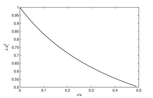
Figure 5: Plots of the quadrature variance of the cavity mode [Eq. (69)] versus $\varepsilon/\kappa$ for $\gamma_{c}/\kappa=0.01$.

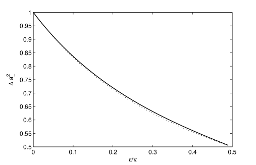
Figure 6: Plots of the quadrature variance of the signal light [Eq. (71)] versus $\varepsilon/\kappa$ in the presence of the two-level atom with $\gamma_{c}/\kappa=0.01$ (solid curve) and in the absence of the two-level atom, i.e, for $\gamma_{c}=0$ (dotted curve).

On the other hand, using (67) and (64), we find the quadrature variance of the signal light to be of the form

$$\Delta\hat{a}_{+}^{2}=1+\frac{(2\varepsilon/\kappa)(1-16\varepsilon^{4}/\kappa^{4}-2\gamma_{c}/\kappa)}{(1-2\varepsilon/\kappa)(1-16\varepsilon^{4}/\kappa^{4})}$$ (70)

and

$$\Delta\hat{a}_{-}^{2}=1-\frac{(2\varepsilon/\kappa)(1-16\varepsilon^{4}/\kappa^{4}-2\gamma_{c}/\kappa)}{(1+2\varepsilon/\kappa)(1-16\varepsilon^{4}/\kappa^{4})}.$$ (71)

We note that $16\varepsilon^{4}/\kappa^{4}=(2\varepsilon/\kappa)^{4}<2\varepsilon/\kappa<1$ and with $\gamma_{c}/\kappa$ being of the order of 0.01, we assert that $1-16\varepsilon^{4}/\kappa^{4}-2\gamma_{c}/\kappa$ is positive. We then see that for the signal light $\Delta a_{+}^{2}>1$ and $\Delta a_{-}^{2}<1$ and hence the squeezing occurs in the minus quadrature. In Fig. 6, we plot Eq. (71) versus $\varepsilon/\kappa$ in the presence and in the absence of the two-level atom. We see from this figure that the degree of squeezing of the signal light slightly decreases due to the presence of the two-level atom. We also see that the degree of squeezing increases as $\varepsilon/\kappa$ increases. It is well known that the signal light consists of highly correlated pairs of photons and this correlation is responsible for the squeezing of this light. Since the two-level atom absorbs a single photon at a time, it somewhat destroys the correlations between signal photon pairs. This leads to the decrease in the degree of squeezing of the signal light.

It is also interesting to check if the fluorescent light emitted by the two-level atom is in a squeezed state. To this end, applying Eqs. (67) and (65) the quadrature variance of the fluorescent light can be expressed as

$$\Delta\hat{a}_{+}^{2}=1+\frac{2\gamma_{c}\varepsilon/\kappa^{2}}{(1-2\varepsilon/\kappa)(1-4\varepsilon^{2}/\kappa^{2})}$$ (72)

and

$$\Delta\hat{a}_{-}^{2}=1-\frac{2\gamma_{c}\varepsilon/\kappa^{2}}{(1+2\varepsilon/\kappa)(1-4\varepsilon^{2}/\kappa^{2})}.$$ (73)

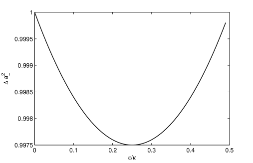
Figure 7: Plots of the quadrature variance of the fluorescent light [Eq. (73)] versus $\varepsilon/\kappa$ for $\gamma_{c}/\kappa=0.01$.

We note from this result that the fluorescent light is in a squeezed state. Fig. 7 indicates that the degree of squeezing of the fluorescent light is very small.

V power spectrum of the cavity mode

We finally determine the power spectrum of the cavity mode. The power spectrum of the cavity mode can be expressed as

$$S(\omega)=2Re\int_{0}^{\infty}\langle\hat{a}^{\dagger}(t)\hat{a}(t+\tau)\rangle_{ss}e^{i\omega\tau}d\tau.$$ (74)

With the aid of Eqs. (6b) and (7a), we easily get

$$\frac{d}{dt}\langle\hat{a}\rangle=-\frac{\kappa}{2}\langle\hat{a}\rangle+\varepsilon\langle\hat{a}^{\dagger}\rangle-g\langle\hat{\sigma}_{-}\rangle.$$ (75)

Applying (75) and its complex conjugate, one can write

$$\frac{d}{dt}\alpha_{\pm}=-\mu_{\mp}\alpha_{\pm}-gz_{\pm},$$ (76)

in which $\mu_{\mp}=\kappa(\frac{1}{2}\mp\frac{\varepsilon}{\kappa})$ and $\alpha_{\pm}=\langle\hat{a}\rangle\pm\langle\hat{a}^{\dagger}\rangle$. A formal solution of this equation can be written as

$$\alpha_{\pm}(t+\tau)=\alpha_{\pm}(t)e^{-\mu_{\mp}\tau}-g~{}e^{-\mu_{\mp}\tau}\int_{0}^{\tau}e^{\mu_{\mp}\tau^{\prime}}z_{\pm}(t+\tau^{\prime})d\tau^{\prime},$$ (77)

so that on account of Eq. (27), we have

$$\alpha_{\pm}(t+\tau) =\alpha_{\pm}(t)e^{-\mu_{\mp}\tau}-g~{}z_{\pm}(t)e^{-\mu_{\mp}\tau}$$

$$\times\int_{0}^{\tau}e^{-(\lambda_{\pm}-\mu_{\mp})\tau^{\prime}}d\tau^{\prime}.$$ (78)

Upon performing the integration, we obtain

$$\alpha_{\pm}(t+\tau)=\alpha_{\pm}(t)e^{-\mu_{\mp}\tau}+\frac{g~{}z_{\pm}(t)}{\lambda_{\pm}-\mu_{\mp}}(e^{-\lambda_{\pm}\tau}-e^{-\mu_{\mp}\tau}).$$ (79)

It then follows that

$$\langle\hat{a}(t+\tau)\rangle =\frac{1}{2}(\langle\hat{a}\rangle+\langle\hat{a}^{\dagger}\rangle)e^{-\mu_{-}\tau}+\frac{1}{2}(\langle\hat{a}\rangle-\langle\hat{a}^{\dagger}\rangle)e^{-\mu_{+}\tau}$$

$$+g\frac{\langle\hat{\sigma}_{-}\rangle+\langle\hat{\sigma}_{+}\rangle}{2(\lambda_{+}-\mu_{-})}(e^{-\lambda_{+}\tau}-e^{-\mu_{-}\tau})$$

$$+g\frac{\langle\hat{\sigma}_{-}\rangle-\langle\hat{\sigma}_{+}\rangle}{2(\lambda_{-}-\mu_{+})}(e^{-\lambda_{-}\tau}-e^{-\mu_{+}\tau}).$$ (80)

and application of the quantum regression theorem leads to

$$\langle\hat{a}^{\dagger}(t)\hat{a}(t+\tau)\rangle_{ss} =N_{1}e^{-\mu_{-}\tau}+N_{2}e^{-\mu_{+}\tau}$$

$$+N_{3}e^{-\lambda_{+}\tau}+N_{4}e^{-\lambda_{-}\tau},$$ (81)

where

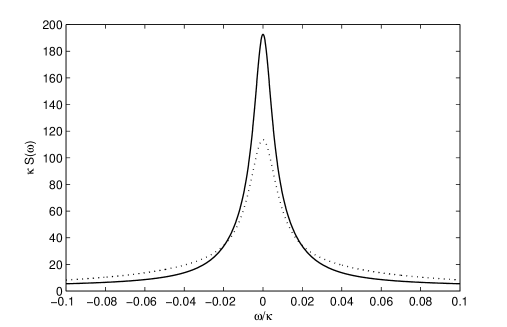
Figure 8: Plots of the power spectrum of the cavity mode [Eq. (V)] versus $\omega/\kappa$ for $\gamma_{c}/\kappa=0.01$, for $\varepsilon/\kappa=0.25$ (solid curve) and for $\varepsilon/\kappa=0.35$ (dotted curve).

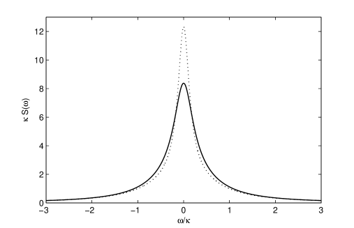
Figure 9: Plot of the power spectrum of the signal light [Eq. (84)] versus $\omega/\kappa$ for $\varepsilon/\kappa=0.25$ (solid curve) and for $\varepsilon/\kappa=0.35$ (dotted curve).

$$N_{1}=\frac{1}{2}(\langle\hat{a}^{\dagger}\hat{a}\rangle_{ss}+\langle\hat{a}^{\dagger 2}\rangle_{ss}+\frac{g}{2}\frac{\langle\hat{a}^{\dagger}\hat{\sigma}_{-}\rangle_{ss}+\langle\hat{a}^{\dagger}\hat{\sigma}_{+}\rangle_{ss}}{\lambda_{+}-\mu_{-}})$$

$$N_{2}=\frac{1}{2}(\langle\hat{a}^{\dagger}\hat{a}\rangle_{ss}-\langle\hat{a}^{\dagger 2}\rangle_{ss}+\frac{g}{2}\frac{\langle\hat{a}^{\dagger}\hat{\sigma}_{-}\rangle_{ss}-\langle\hat{a}^{\dagger}\hat{\sigma}_{+}\rangle_{ss}}{\lambda_{-}-\mu_{+}})$$

$$N_{3}=\frac{g}{2}\frac{\langle\hat{a}^{\dagger}\hat{\sigma}_{-}\rangle_{ss}+\langle\hat{a}^{\dagger}\hat{\sigma}_{+}\rangle_{ss}}{\lambda_{+}-\mu_{-}}$$

$$N_{4}=\frac{g}{2}\frac{\langle\hat{a}^{\dagger}\hat{\sigma}_{-}\rangle_{ss}-\langle\hat{a}^{\dagger}\hat{\sigma}_{+}\rangle_{ss}}{\lambda_{-}-\mu_{+}}.$$ (82)

On account of (V), the normalized power spectrum of the cavity mode turns out to be

$$S(\omega) =\frac{\kappa(\frac{1}{2}+\frac{\varepsilon}{\kappa})/4\pi}{\kappa^{2}(\frac{1}{2}+\frac{\varepsilon}{\kappa})^{2}+\omega^{2}}+\frac{\kappa(\frac{1}{2}-\frac{\varepsilon}{\kappa})/4\pi}{\kappa^{2}(\frac{1}{2}-\frac{\varepsilon}{\kappa})^{2}+\omega^{2}}$$

$$+\frac{\Gamma(\frac{1}{2}+\frac{\varepsilon}{\kappa})/4\pi}{\Gamma^{2}(\frac{1}{2}+\frac{\varepsilon}{\kappa})^{2}+\omega^{2}}+\frac{\Gamma(\frac{1}{2}-\frac{\varepsilon}{\kappa})/4\pi}{\Gamma^{2}(\frac{1}{2}-\frac{\varepsilon}{\kappa})^{2}+\omega^{2}}.$$ (83)

We identify that

$$S(\omega)=\frac{\kappa(\frac{1}{2}+\frac{\varepsilon}{\kappa})/2\pi}{\kappa^{2}(\frac{1}{2}+\frac{\varepsilon}{\kappa})^{2}+\omega^{2}}+\frac{\kappa(\frac{1}{2}-\frac{\varepsilon}{\kappa})/2\pi}{\kappa^{2}(\frac{1}{2}-\frac{\varepsilon}{\kappa})^{2}+\omega^{2}}$$ (84)

is the power spectrum of the signal light. The last two terms in Eq. (V) represent the power spectrum of the fluorescent light, which is the same as Eq. (35). Since the expression for the spectrum of the signal light does not contain $\gamma_{c}$, the presence of the two-level atom does not affect the width of this spectrum. In Fig. 8, we plot the power spectrum of the cavity mode versus $\omega/\kappa$ for different values of $\varepsilon/\kappa$. These plots show that the width of the power spectrum increases as the degree of squeezing increases. When the value of $\varepsilon/\kappa$ increases from $0.25$ to $0.35$, the half width increases from $0.0072$ to $0.0108$. In addition, in Fig. 9 we plot the power spectrum of the signal light versus $\omega/\kappa$ for different values of $\varepsilon/\kappa$. These plots indicate that the width of the spectrum decreases as the degree of squeezing increases. The half width of the spectrum decreases from 0.3168 to 0.1766 as $\varepsilon/\kappa$ increases from 0.25 to 0.35.

VI Conclusion

We have studied a degenerate parametric oscillator with a two-level atom applying the Heisenberg and quantum Langevin equations in the bad-cavity limit. We have obtained the mean photon number, the quadrature variance, and the power spectrum for the cavity mode, for the signal light, and for the fluorescent light. In addition, we have determined the second-order correlation function for the fluorescent light. The method we have used enables us to investigate both the atomic fluorescence and the quantum statistical properties of the cavity mode.

We have found that the photons in the fluorescent light are antibunched. Unlike the power spectrum of the fluorescent light from a two-level atom driven by a strong coherent light, the power spectrum of the fluorescent light in this case turns out to be a single peak. It is found that the width of the spectrum increases with $\varepsilon/\kappa$. Moreover, we have seen that the fluorescent light is in a squeezed state with a very small amount of squeezing.

On the other hand, the presence of the two-level atom leads to a decrease in the mean photon number and in the degree of squeezing of the signal light. However, the presence of the two-level atom has no effect on the spectrum of the signal light.

References

(1)A.S. Parkins, Phys. Rev. A 42, (1990) 4352.
(2)J.I. Cirac, L.L. Sanchez-Soto, Phys. Rev. A 44, (1991) 1948.
(3)J.I. Cirac, Phys. Rev. A 46, (1992) 4354.
(4)P.R. Rice, L.M. Pedrotti, J. Opt. Soc. Am. B 9, (1992) 2008.
(5)P.R. Rice, C.A. Baird, Phys. Rev. A 53, (1996) 3633.
(6)W.S. Smyth, S. Swain, Phys. Rev. A 53, (1996) 2846.
(7)D. Erenso, R. Vyas, Phys. Rev. A 65, (2002) 063808.
(8)G. S. Agarwal, Phys. Rev. A 40, (1989) 4138.
(9)S. Jin, Min Xiao, Phys. Rev. A 49, (1994) 499.
(10)J.P. Clemens, P.R. Rice, P.K. Rungta, and R.J. Brecha, Phys. Rev. A 62, (2000) 033802.