Electronic Noise in Optical Homodyne Tomography
Abstract
The effect of the detector electronic noise in an optical homodyne tomography experiment is shown to be equivalent to an optical loss if the detector is calibrated by measuring the quadrature noise of the vacuum state. An explicit relation between the electronic noise level and the equivalent optical efficiency is obtained and confirmed in an experiment with a narrowband squeezed vacuum source operating at an atomic rubidium wavelength.
pacs:
42.50.Dv,03.65.Wj,05.40.CaIntroduction
Optical homodyne tomography (OHT) is a method of characterizing quantum states of light by measuring the quantum noise statistics of the electromagnetic field quadratures at different phases. Theoretically proposed in VogelRisken and first experimentally implemented in the early 1990s smi93a , OHT has become a standard tool of quantum technology of light, in particular in quantum information applications.
OHT is prone to a variety of inefficiencies, of which the main one — the optical losses (OLs) — is due to absorption in beam paths, non-unitary efficiency of the photodiodes, imperfect balancing of the detector, and, partially, imperfect mode matching between the signal and the local oscillator modes ray95 . Also, the presence of non-mode-matched signal light appears as added noise in the detector, raising the apparent noise floor ray95 . All OLs can be modeled by an absorber in the signal beam path. The effect of OL in quantum state reconstruction is well understood, and there are ways of both its quantitative evaluation and compensation for its effects in the quantum state reconstruction procedure leonhardt ; kiss95 .
An important additional inefficiency source is the electronic noise (EN) of the homodyne detector. Its effect is the addition of a random value to each quadrature measurement, which blurs the marginal distribution and causes errors in quantum state reconstruction. Unlike the optical inefficiency, the EN, to our knowledge, has not yet been studied, and is usually neglected whenever an efficiency analysis is made smi92 ; Fock ; DispFock ; QubitHT ; our06 ; Fock2 ; nee06 .
The purpose of this paper is to fill this gap and to analyze the role of the electronic noise in OHT. We show its effect to be equivalent to that of optical losses. The key to this equivalence is the detector calibration procedure, which involves measuring the quadrature noise of the vacuum state. Applying this procedure to the vacuum state contaminated with the EN results in rescaling of the field quadratures, analogous to that taking place due to optical absorption.
We confirm our experimental findings in a squeezing experiment, in which we vary the local oscillator power to achieve different signal-to-noise ratios of the homodyne detector. The squeezed vacuum source is a narrowband, tunable continuous-wave optical parametric amplifier operating at a 795-nm wavelength.
We begin our theory by writing the effects of both inefficiency types on the reconstructed Wigner function (WF).
The beam splitter model for optical signal loss
According to the beam splitter model of absorption, non-unitary optical efficiency modifies the WF of the signal state as follows leonhardt :
This transformation can be understood by visualizing the absorber as a fictional beam splitter with the signal beam entering one port and the vacuum state entering the other. Transmission of the signal field through the beam splitter rescales the field amplitudes by a factor of . The vacuum state reflected from the beam splitter into the signal mode adds noise, which expresses as a convolution of the WF with a two-dimensional Gaussian function of width .
Effect of the electronic noise
In the absence of the electronic noise, the electric signal (voltage or current) generated by the homodyne detector is proportional to the quadrature sample : . The coefficient has to be determined when quantum state reconstruction is the goal. This is usually done by means of a calibration procedure, which consists of acquiring a set of quadrature noise samples of the vacuum state, prepared by letting only the local oscillator into the detector. The vacuum marginal distribution,
| (2) |
is loss-independent, and has a mean square of . One can thus use the experimental data to obtain
| (3) |
When the EN is present, the observed probability distribution of the electric signal is a convolution of the scaled marginal distribution of the state measured and the electronic noise histogram :
| (4) |
(the factor of is added to retain the normalization of the marginal distribution). Under realistic experimental conditions of a broadband electronic noise, its distribution can be assumed Gaussian:
| (5) |
where is the mean square noise magnitude.
Consider the detector calibration procedure in the presence of the EN. According to Eqs. (2), (4), and (5), the vacuum state measurement yields a distribution
| (6) |
with a mean square of . If no correction for the EN is made, the quantity
| (7) |
is interpreted according to Eq. (3) as the conversion factor between the electric signal and the field quadrature.
In a homodyne measurement of an unknown state, one acquires a set of samples from the homodyne detector, and then applies the calibration factor to rescale its histogram and obtain the associated marginal distribution. Using Eq. (4), we write
Introducing a new integration variable and utilizing the EN distribution (5), Eq. (Effect of the electronic noise) can be rewritten as
This rescaled, noise contaminated marginal distribution is then used to reconstruct the Wigner function.
Because the marginal distribution is tomographically linked to the WF,
| (10) |
the Wigner function reconstructed from a noisy measurement is a convolution
| (11) | |||||
Equivalence of the efficiency loss mechanisms
Comparing the above expression with Eq. (The beam splitter model for optical signal loss) for the WF of a state affected by optical losses, we find that the two are equivalent if we set
| (12) |
In other words, we may treat the electronic noise as an additional optical attenuator with a transmission equal to . Accordingly, the known numerical procedures for correcting for optical losses can be readily applied to the electronic noise.
This result may appear surprising. The field quadrature noise measured in the presence of the EN is a convolution of the WF’s marginal distribution with the noise histogram. In the case of OL, on the other hand, the convolution is preceded by rescaling of the quadrature variables. The similarity between the effects of the two inefficiency emerges due to the detector calibration procedure. The vacuum state measurement is distorted by the EN but not the OL, hence there is additional rescaling of the quadratures in the presence of the EN.
For experimental applications, it is more convenient to express the equivalent efficiency in terms of the signal-to-noise ratio of the detector. By the latter we understand the ratio between the observed mean square noise of the vacuum state (in the presence of the EN) and the mean square electronic noise, i.e. the quantity
| (13) |
Re-expressing Eq. (12) in terms of yields
| (14) |
As evidenced by this equation, reasonably low electronic noise does not constitute a significant efficiency loss. For example, the original time-domain detector of Smithey and co-workers smi92 ; smi93a , featuring a 6 dB signal-to-noise ratio (i.e. the rms quadrature noise being only twice as high as the rms EN) has an equivalent quantum efficiency of 75%. A similar equivalent efficiency is featured by a high-speed detector by Zavatta et al. ZavattaHD . A 14-dB time-domain detector of Hansen and co-workers HansenHD has an equivalent efficiency of 96%, and a typical frequency-domain detector with a signal-to-noise ratio of 20 dB has an efficiency of 99%.
Experiment
We verify our theoretical findings in a squeezing experiment. The squeezed vacuum source is a continuous-wave optical parametric amplifier (OPA), operating at the 795-nm wavelength of the D1 transition in atomic rubidium. We have constructed this source to perform experiments on interfacing quantum information between light and atoms, in particular storage kuzmich:05 ; lukin:05 and Raman adiabatic transferring appel:06 ; vewinger-2006 of light in atomic vapor. Similar sources have been reported very recently by two groups tanimura-2006 ; hetet-2006
The optical cavity of the OPA is of bow-tie configuration composed of four mirrors, among which two are flat and two are concave with a curvature radius of 100 mm. The cavity is singly resonant for the generated 795-nm wavelength. As the output coupler we use one of the flat cavity mirrors, which had a reflectivity of 93%. Other cavity mirrors had an over 99.9% reflectivity. With these parameters, the cavity had a 460-MHz three free spectral range with the resonant line width of 6 MHz
The source employs a 5-mm long periodically poled KTiOPO4 crystal as the nonlinear element. The crystal, manufactured by Raicol, features a 3.175 m poling period and double antireflection coating on both sides. It is placed at the beam waist between the curved mirrors.
The OPA is pumped by up to 240 mW of 397.5 nm light. The pump field is the second harmonic of a frequency stabilized titanium-sapphire master laser. The same laser is used to provide the local oscillator for the homodyne detector. The OPA cavity is locked at resonance by means of an additional diode laser phase locked to the master oscillator at 3 free spectral ranges of the OPA cavity. The cavity lock is implemented using the Pound-Drever-Hall method, using a beam modulated at 20 MHz and propagating in the direction opposite to the pumped mode.
The circuit for homodyne detection uses two Hamamatsu S3883 photodiodes of 94% quantum efficiency in a “back-to-back" configuration, akin to that employed in Refs. HansenHD ; ZavattaHD , followed by a OPA847 operational preamplifier. The detector exhibits excellent linearity and an up to 12-17 dB signal-to-noise ratio over a 100-MHz bandwidth, with local oscillator powers up to 10 mW. At a 1-MHz sideband relevant for this experiment, the highest signal-to-noise ratio of the detector exceeds 17 dB, which, according to Eq. (14), corresponds to equivalent optical losses of only 2%. The detector output is observed in the frequency domain using an Agilent ESA spectrum analyzer.
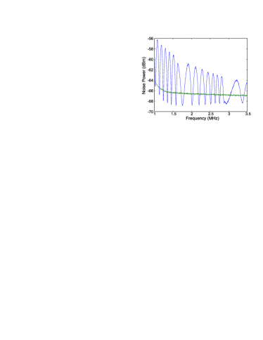
Figure 1 shows the electronic spectrum of squeezed vacuum field generated by the OPA. Up to 3 dB of squeezing is observed within the cavity linewidth.
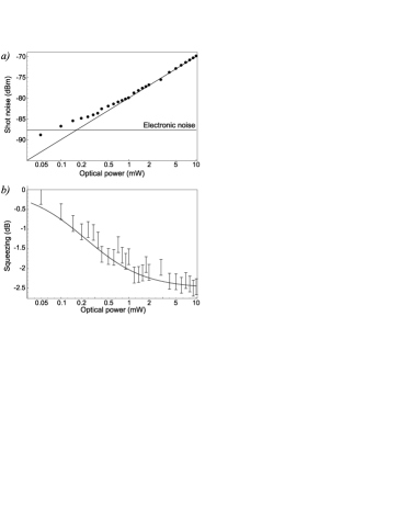
To verify the predictions of Eq. (14), we stabilize the pump level at 140 mW and set the spectrum analyzer to run in the zero span mode at a detection frequency of 1 MHz. The signal-to-noise ratio of the detector is varied by changing the local oscillator intensity. At each intensity value, we record three spectrum analyzer traces: electronic noise (measured by blocking both photodiodes of the homodyne detector), shot noise (measured by blocking the squeezed vacuum signal) and the phase-dependent squeezed vacuum quadrature. The highest () and lowest () quadrature noise levels of the squeezing measurement are then determined and normalized to the shot noise level. The uncertainty of is estimated as 0.2 dB; it is much smaller for the shot-noise and electronic-noise data. The results of these measurements are shown in Fig. 2.
To determine the quantum efficiency, we use the fact that for the pure squeezed state, the product of the mean square quadrature uncertainties is the minimum allowed by the uncertainty principle, i.e. , where the normalization factor corresponds to the shot noise level. After undergoing an optical loss, the squeezed state remains Gaussian, but loses its purity. Using the beam splitter model of absorption, we find that upon propagating through an attenuator of transmission , the quadrature noise reduces by a factor of , but gains excess vacuum noise of intensity :
| (15a) | |||
| (15b) | |||
Measuring and and solving Eqs. (15), we can find the value of , i.e. how much loss a pure squeezed state would have experienced to generate the state with the quadrature noise levels observed lwb06b :
| (16) |
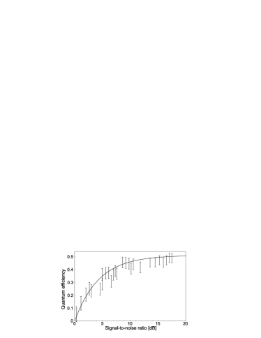
The result of applying this method to our squeezed vacuum data is displayed in Fig. 3 along with a fit with Eq. (14) multiplied by an overall efficiency factor of 0.51 (emerging due to various optical losses). The experimental data matches well to the theoretical prediction.
Conclusion
We have found that there is a strong similarity between the effects of optical absorption and electronic noise on the state reconstructed by means of optical homodyne tomography. Therefore, the detector’s Gaussian electronic noise can be treated as an additional optical loss which is related to the detector’s signal-to-noise ratio by Eq. (14). The finding is verified in a squeezing experiment involving a narrowband nonclassical light source suitable for experiments on interfacing quantum information between light and atoms.
Acknowledgements
We thank Michael Raymer for discussions. A. L.’s research is supported by QuantumWorks, NSERC, CFI, AIF, and CIAR.
References
- (1) K. Vogel and H. Risken, Phys. Rev. A 40, 2847 (1989).
- (2) D. T. Smithey, M. Beck, M. G. Raymer, and A. Faridani, Phys. Rev. Lett. 70, 1244 (1993).
- (3) M. Raymer, J. Cooper, H. Carmichael, M. Beck, and D. Smithey, J. Opt. Soc. of Am. B 12, 1801 (1995).
- (4) U. Leonhardt, Measuring the Quantum State of Light (Cambridge University Press, 1997), pp. 79–81.
- (5) T. Kiss, U. Herzog, and U. Leonhardt, Phys. Rev. A 52, 2433 (1995).
- (6) D. T. Smithey, M. Beck, M. Belsley, and M. G. Raymer, Phys. Rev. Lett. 69, 2650 (1992).
- (7) A. I. Lvovsky et al., Phys. Rev. Lett. 87, 050402 (2001).
- (8) A. I. Lvovsky and S. Babichev, Phys. Rev. A 66, 11801 (2002).
- (9) S. A. Babichev, J. Appel, and A. I. Lvovsky, Phys. Rev. Lett. 92, 193601 (2004).
- (10) A. Ourjoumtsev, R. Tualle-Brouri, J. Laurat, and P. Grangier, Science 312, 83 (2006).
- (11) A. Ourjoumtsev, R. Tualle-Brouri, and P. Grangier, Phys. Rev. Lett. 96, 213601 (2006).
- (12) J. S. Neergaard-Nielsen, B. M. Nielsen, C. Hettich, K. Mølmer, and E. S. Polzik, Phys. Rev. Lett. 97, 083604 (2006).
- (13) A. Zavatta, M. Bellini, P. L. Ramazza, F. Marin, and F. T. Arecchi, J. Opt. Soc. Am. B 19, 1189 (2002).
- (14) H. Hansen et al., Opt. Lett. 26, 1714 (2001).
- (15) T. Chaneliere et al., Nature 438, 833 (2005).
- (16) M. Eisaman et al., Nature 438, 837 (2005).
- (17) J. Appel, K.-P. Marzlin, and A. I. Lvovsky, Phys. Rev. A 73, 013804 (2006).
- (18) F. Vewinger, J. Appel, E. Figueroa, and A. I. Lvovsky, quant-ph/0611181 .
- (19) T. Tanimura, D. Akamatsu, Y. Yokoi, A. Furusawa, and M. Kozuma, Opt. Lett. 31, 2344 (2006).
- (20) G. Hetet et al., J. Phys. B 40, 221 (2007).
- (21) A. I. Lvovsky, W. Wasilewski, and K. Banaszek, quant-ph/0601170 .