myctr

CHARACTERIZING AND MEASURING MULTIPARTITE ENTANGLEMENT

Abstract

A method is proposed to characterize and quantify multipartite entanglement in terms of the probability density function of bipartite entanglement over all possible balanced bipartitions of an ensemble of qubits. The method is tested on a class of random pure states.

The quantification of multipartite entanglement is an open and very challenging problem. An exhaustive definition of bipartite entanglement exists and hinges upon the von Neumann entropy and the entanglement of formation,[1] but the problem of defining multipartite entanglement is more difficult[2] and no unique definition exists: different definitions tend indeed to focus on different aspects of the problem, capturing different features of entanglement,[3] that do not necessarily agree with each other. Moreover, as the size of the system increases, the number of measures (i.e. real numbers) needed to quantify multipartite entanglement grows exponentially.

This work is motivated by the idea that a good definition of multipartite entanglement should stem from some statistical information about the system.[4] We shall therefore look at the distribution of the purity of a subsystem over all bipartitions of the total system. As a measure of multipartite entanglement we will take a whole function: the probability density of bipartite entanglement between any two parts of the total system. According to our definition multipartite entanglement is large when bipartite entanglement (i) is large and (ii) does not depend on the bipartition, namely when (i$+$ii) the probability density of bipartite entanglement is a narrow function centered at a large value. This definition will be tested on two class of states that are known to be characterized by a large entanglement. We emphasize that the idea that complicated phenomena cannot be “summarized” in a single (or a few) number(s) was already proposed in the context of complex systems[5] and has been also considered in relation to quantum entanglement.[6]

We shall focus on a collection of $n$ qubits and consider a partition in two subsystems $A$ and $B$, made up of $n_{A}$ and $n_{B}$ qubits ($n_{A}+n_{B}=n$), respectively. For definiteness we assume $n_{A}\leq n_{B}$. The total Hilbert space is the tensor product $\mathcal{H}=\mathcal{H}_{A}\otimes\mathcal{H}_{B}$ and the dimensions are $\dim\mathcal{H}=N=2^{n}$, $\dim\mathcal{H}_{A}=N_{A}=2^{n_{A}}$ and $\dim\mathcal{H}_{B}=N_{B}=2^{n_{B}}$, respectively ($N_{A}N_{B}=N$).

We shall consider pure states. Their expression adapted to the bipartition reads

$$|\psi\rangle=\sum_{k=0}^{N-1}z_{k}|k\rangle=\sum_{j_{A}=0}^{N_{A}-1}\sum_{l_{B}=0}^{N_{B}-1}z_{j_{A}l_{B}}|j_{A}\rangle\otimes|l_{B}\rangle,$$ (1)

where $|k\rangle=|j_{A}\rangle\otimes|l_{B}\rangle$, with a bijection between $k$ and $(j_{A},l_{B})$. Think of the binary expressions of an integer $k$ in terms of the binary expression of $(j_{A},l_{B})$.

As a measure of bipartite entanglement between $A$ and $B$ we consider the participation number

$$N_{AB}=\pi_{AB}^{-1},\qquad\pi_{AB}(|\psi\rangle)=\mathrm{tr}_{A}\rho_{A}^{2},\qquad\rho_{A}=\mathrm{tr}_{B}\rho,$$ (2)

where $\rho=|\psi\rangle\langle\psi|$ and $\mathrm{tr}_{A}$ ($\mathrm{tr}_{B}$) is the partial trace over the subsystem $A$ ($B$). $N_{AB}$ measures the effective rank of the matrix $\rho_{A}$, namely the effective Schmidt number.[7] We note that

$$1\leq N_{AB}=N_{BA}\leq\text{min}(N_{A},N_{B}),$$ (3)

with the maximum (minimum) value attained for a completely mixed (pure) state $\rho_{A}$. Therefore, a larger value of $N_{AB}$ corresponds to a more entangled bipartition $(A,B)$, the maximum value being attainable for a balanced bipartition, i.e. when $n_{A}=[n/2]$ (and $n_{B}=[(n+1)/2]$), where $[x]$ is the integer part of the real $x$, that is the largest integer not exceeding $x$. The maximum possible entanglement is $N_{AB}=N_{A}=2^{n_{A}}$. The quantity $n_{AB}=\log_{2}N_{AB}$ represents the effective number of entangled qubits, given the bipartition (namely, the number of bipartite entanglement “links” that are “severed” when the system is bipartitioned).

Clearly, the quantity $N_{AB}$ will depend on the bipartition, as in general entanglement will be distributed in a different way among all possible bipartitions. As explained in the introduction, we are motivated by the idea that the distribution $p(N_{AB})$ of $N_{AB}$ yields information about multipartite entanglement.

Let us therefore study the typical form of our measure of multipartite entanglement $p(N_{AB})$ for a very large class of pure states, sampled according to a given symmetric distribution on the projective Hilbert space $\{\psi\in\mathcal{H},\|\psi\|=1\}$ (e.g. the unitarily invariant Haar measure). By plugging (1) into (2) one gets

$$\pi_{AB}=\sum_{j,j^{\prime}=0}^{N_{A}-1}\,\sum_{l,l^{\prime}=0}^{N_{B}-1}z_{jl}\bar{z}_{j^{\prime}l}z_{j^{\prime}l^{\prime}}\bar{z}_{jl^{\prime}}$$ (4)

and it can be shown[4] that, in the thermodynamical limit (that is practically attained for $n>5$), independently of the distribution of the coefficients, the mean and the standard deviation of (4) over all possible balanced bipartitions read

$$\mu_{AB}=\frac{N_{A}+N_{B}-1}{N}=\sqrt{\frac{\alpha}{N}}\,,\quad\sigma^{2}_{AB}=\frac{2}{N^{2}},\quad(N\;\mbox{large})$$ (5)

respectively, where $\alpha=8/2$ $(\alpha=9/2)$ for even (odd) $n$. Moreover, the probability density of $N_{AB}$ in Eq. (2) reads

$$p(N_{AB}) = \frac{1}{N^{2}_{AB}(2\pi\sigma_{AB}^{2})^{1/2}}\exp\left(-\frac{(N_{AB}^{-1}-\mu_{AB})^{2}}{2\sigma_{AB}^{2}}\right).$$ (6)

It is interesting to compare the features of these generic random states with those of other states studied in the literature.

Mean bipartite entanglement $\langle N_{AB}\rangle$ for different states and different number of qubits $n$. $n$ GHZ W cluster random 5 2 1.923 3.6 2.909 6 2 2 5.4 4.267 7 2 1.96 6.171 5.565 8 2 2 8.743 8.258 9 2 1.976 10.349 10.894 10 2 2 14.206 16.254 11 2 1.984 17.176 21.558 12 2 2 23.156 32.252

Table CHARACTERIZING AND MEASURING MULTIPARTITE ENTANGLEMENT displays the average value of $N_{AB}$ for GHZ states,[8] W states,[9] cluster states[10] and the generic states (1), for $n=5\div 12$. While the entanglement of the GHZ and W states is essentially independent of $n$, the situation is drastically different for cluster and random states. In both cases, the average entanglement increases with $n$; for $n>8$ the average entanglement is higher for random states. However, the mean $\langle N_{AB}\rangle$ yields poor information on multipartite entanglement. For this reason, it is useful to analyze the distribution of bipartite entanglement over all possible balanced bipartitions.

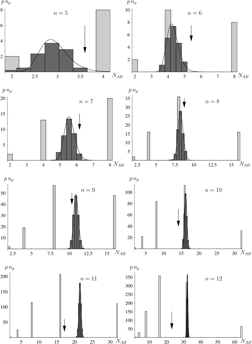
Figure 1: Number of balanced bipartitions vs $N_{AB}$; $n_{p}=n!/n_{A}!n_{B}!$ is the number of bipartitions. the light-gray bars represent cluster states, the dark-gray ones random states; the solid line is the distribution (5)-(6); the black arrows indicate the average $\langle N_{AB}\rangle_{\text{cluster}}$. For even $n$ ($n=12$ in particular) the distribution of the random state partially hides a peak of the corresponding cluster state distribution, centered at $N_{AB}=2^{n_{A}-1}=2^{[n/2]-1}$.

The results for the cluster and random states are shown in Fig. 1, for $n$ ranging between 5 and 12. Notice that the distribution function of the random state is always peaked around $\langle N_{AB}\rangle\simeq\mu_{AB}^{-1}$ given by (5). Notice also that the cluster state can reach higher values of $N_{AB}$ (the maximum possible value being $2^{[n/2]}$), however, the fraction of bipartitions yielding this result becomes smaller for higher $n$. This is immediately understood if one realizes that the cluster states are designed for optimized applications and therefore perform better in terms of specific bipartitions. On the other hand, according to the measure we propose, the random states are characterized by a large value of multipartite entanglement, that is roughly independent of the bipartition.

In Fig. 2 we compare the number of balanced bipartitions vs $N_{AB}$ for the random states and increasing $n$. The related probability density functions (6) are displayed in Fig. 3. Notice that as the number of spins increases from $n=5$ to $n=12$ the mean increases and the distribution becomes relatively narrower. As we emphasized, these are both signatures of a very high degree of multipartite entanglement, whose features become (as $n$ increases) practically independent of the bipartition. In Fig. 3 it is interesting to observe the difference between the distributions for odd and even $n$.

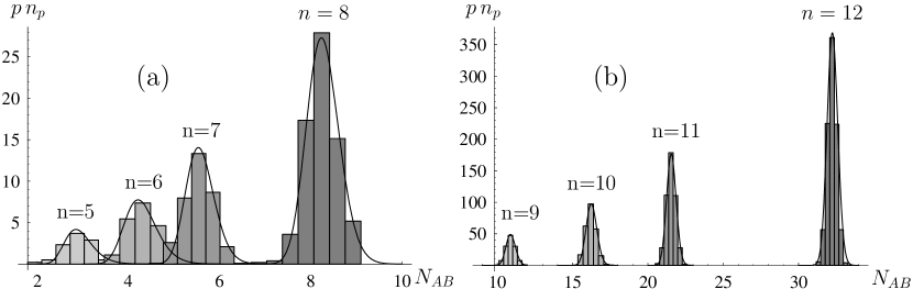
Figure 2: Number of balanced bipartitions vs $N_{AB}$; the histograms are numerically obtained for the typical states; the solid line represents their distribution. The value of $n$ (total number of spins) is always indicated and ranges (a) from 5 to 8; (b) from 9 to 12; $n_{p}=n!/n_{A}!n_{B}!$ is the number of bipartitions.

Figure 3: Probability densities functions (6) vs $N_{AB}$. Each curve is labeled with the corresponding value of $n$ (number of qubits). The standard deviation $\sigma$ quickly becomes independent of $n$ [see Fig. 4(b)] and depends only on parity of the latter.

In Fig. 4(a) we plot the value of $\langle N_{AB}\rangle$ for the cluster and random states (see Table CHARACTERIZING AND MEASURING MULTIPARTITE ENTANGLEMENT). We notice that, for $n=9$, $\langle N_{AB}\rangle_{\text{random}}$ becomes larger than $\langle N_{AB}\rangle_{\text{cluster}}$. Figure 4(b) displays the behavior of the standard deviation of $N_{AB}$,

$$\sigma\simeq\sigma_{AB}/\mu_{AB}^{2}.$$ (7)

For the cluster states this quantity tends to diverge when the size of the system increases. By contrast, from Eq. (5), $\sigma=\sqrt{2}/\alpha$ is constant for the typical states. This means that the ratio $\sigma/\langle N_{AB}\rangle$ tends to 0.

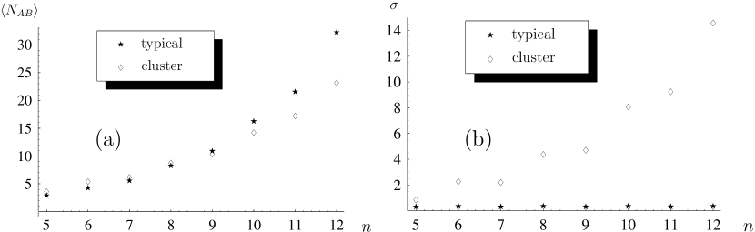
Figure 4: Comparison between typical and cluster states: (a) expectation value $\langle N_{AB}\rangle$ and (b) standard deviation $\sigma$ of the distributions in Fig. 3 vs $n$ (number of qubits).

Finally, Figure 5 displays a parametric plot of $\sigma$ vs $\langle N_{AB}\rangle$. Clearly, for the random states $\sigma$ is independent of $\langle N_{AB}\rangle$.

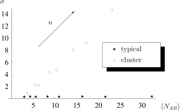
Figure 5: Standard deviation $\sigma$ vs expectation value $\langle N_{AB}\rangle$ of the distributions in Fig. 3.

We emphasize that our analysis should by no means be taken as an argument against the performance of the cluster states. As we stressed before, cluster states are tailored for specific purposes in quantum information processing, and in that respect are very well suited. We compared the generic states to the cluster states specifically because the latter are also known to be characterized by a large entanglement.

An efficient way to generate states endowed with random features is by means of a chaotic dynamics,[12] or at the onset of a quantum phase transition.[13] In particular, the random states describe quite well states with support on chaotic regions of phase space, before dynamical localization has taken place. These features make these states rather appealing, from a practical point of view, in that they are easily generated. The introduction of a probability density function as a measure of multipartite entanglement paves the way to further investigations of the intimate relation between entanglement and randomness and their behavior across a phase transition.

References

- [1] W. K. Wootters, “Quantum Information and Computation” (Rinton Press, 2001), Vol. 1; C. H. Bennett, D. P. DiVincenzo, J. A. Smolin, and W. K. Wootters, Phys. Rev. A 54, 3824 (1996).
- [2] D. Bruss, J. Math. Phys. 43, 4237 (2002).
- [3] V. Coffman, J. Kundu and W. K. Wootters, Phys. Rev. A 61, 052306 (2000); A. Wong and N. Christensen, Phys. Rev. A 63, 044301 (2001); D.A. Meyer and N.R. Wallach, J. Math. Phys. 43, 4273 (2002).
- [4] P. Facchi, G. Florio and S. Pascazio, quant-ph/0603281 (2006).
- [5] G. Parisi, “Statistical Field Theory” (Addison-Wesley, New York, 1988).
- [6] V. I. Man’ko, G. Marmo, E. C. G. Sudarshan and F. Zaccaria J. Phys. A: Math. Gen. 35, 7137 (2002).
- [7] R. Grobe, K. Rza̧żewski and J.H. Eberly, J. Phys. B 27, L503 (1994).
- [8] D.M. Greenberger, M. Horne and A. Zeilinger, Am. J. Phys. 58, 1131 (1990).
- [9] R. Werner, Phys. Rev. A 40, 4277 (1989); W. Dür, G. Vidal and J.I. Cirac, Phys. Rev. A 62, 062314 (2000).
- [10] H.J. Briegel and R. Raussendorf, Phys. Rev. Lett. 86, 910 (2001).
- [11] E. Lubkin, J. Math. Phys. 19, 1028 (1978); S. Lloyd and H. Pagels, Ann. Phys., NY, 188, 186 (1988); K Życzkowski and H.-J. Sommers J. Phys. A 34, 7111 (2001); A. J. Scott and C. M. Caves, J. Math. Phys. 36, 9553 (2003); Y. Shimoni, D. Shapira and O. Biham, Phys. Rev. A 69, 062303 (2004).
- [12] J. N. Bandyopadhyay and A. Lakshminarayan Phys. Rev. Lett. 89 060402 (2002); S. Montangero, G. Benenti, and R. Fazio, Phys. Rev. Lett. 91, 187901 (2003); S. Bettelli and D. L. Shepelyansky, Phys. Rev. A 67, 054303 (2003); C. Mej a-Monasterio, G. Benenti, G. G. Carlo, and G. Casati, Phys. Rev. A 71, 062324 (2005).
- [13] A. Osterloh, L. Amico, G. Falci, and R. Fazio, Nature 416, 609 (2002); G. Vidal, J. I. Latorre, E. Rico, and A. Kitaev, Phys. Rev. Lett. 90, 227902 (2003); F. Verstraete, M. Popp, and J. I. Cirac, Phys. Rev. Lett. 92, 027901 (2004); T. Roscilde, P. Verrucchi, A. Fubini, S. Haas and V. Tognetti, Phys. Rev. Lett. 93, 167203 (2004).