Non-destructive interferometric characterization of an optical dipole trap

Abstract

A method for non-destructive characterization of a dipole trapped atomic sample is presented. It relies on a measurement of the phase-shift imposed by cold atoms on an optical pulse that propagates through a free space Mach-Zehnder interferometer. Using this technique we are able to determine, with very good accuracy, relevant trap parameters such as the atomic sample temperature, trap oscillation frequencies and loss rates. Another important feature is that our method is faster than conventional absorption or fluorescence techniques, allowing the combination of high-dynamical range measurements and a reduced number of spontaneous emission events per atom.

I Introduction

The first demonstration of optical trapping Chu et al. (1986) of laser cooled atomic samples has paved the way towards non-dissipative traps, with long storage times, as well as optical lattices. This relatively long lifetime is associated with low photon scattering rates in far-off resonant optical traps (FORT), and had made possible to obtain all-optical Bose-Einstein condensates (BEC) Barrett et al. (2001), Weber et al. (2003). Optical lattices have recently been used to form a storage medium for strontium atoms in an optical atom clock Takamoto et al. (2005), that allows for long interrogation times and higher signal-to-noise ratios. On the other hand, considering the field of quantum information and, in particular, the engineering of quantum states, an optical dipole trap provides a medium with a significant atomic density, a necessary condition for the optimal creation of atomic spin squeezed states (SSS) Oblak et al. (2005).

In all of these experiments the characterization of trapped samples is of interest. It has been shown Lye et al. (2003) that, in the case of dense atomic samples, non-invasive detection methods are more powerful than the absorption imaging and fluorescence techniques Kuppens et al. (2000). Non-destructive phase-contrast imaging has already been demonstrated for sodium BEC in a magnetic trap Andrews et al. (1996). The technique of contrast enhancement by implementation of a $\pi/2$ phase-shift between scattered and imaging light is an improved non-destructive dark-ground imaging technique Andrews et al. (1997), where the off-resonant light is used to image the BEC cloud on a CCD. The phase-contrast method has also been applied in a Rabi oscillation experiment of a rubidium BEC where a superposition between two internal states is created Matthews et al. (1999). The spatial heterodyne imaging technique has been used to record the atomic density distribution of a dark-spot MOT in the light interference pattern Kadlecek et al. (2001). A recent work introduces the diffraction-contrast imaging as a non-destructive measurement technique Turner et al. (2005) of cold atoms.

In this paper we present a novel method of non-destructive characterization of optically trapped atomic samples which relies on optical phase-shift measurements in a Mach-Zehnder white-light interferometer, with a sensitivity limited only by the quantum noise of the probe light. The idea behind this interferometric measurement is presented in Oblak et al. (2005) as a tool for creation of squeezed atomic states Kitagawa and Ueda (1993) via a quantum non-demolition measurement (QND) Kuzmich et al. (1998). Because of the very high bandwidth achievable by an interferometric measurement, a system similar to ours is projected to be used for non-destructive real-time stabilization of a BEC Figl et al. (2006). In the presented work we demonstrate that using relatively low power and large detuning, we are able to determine relevant trap parameters as losses, oscillation frequency and temperature of trapped atoms in a measurement procedure that is faster and non-destructive, than the conventional imaging techniques.

The paper is organized as follows. We begin with a short description of the interaction between a polarized light field and an unpolarized atomic sample, followed by the derivation of an equation for the phase-shift in our current experimental scheme. Then we proceed with the theoretical analysis of the noise sources in our free-space white-light Mach-Zehnder interferometer. In the third section we present our experimental apparatus and the results of our trap characterization.

II Theoretical description

II.1 Phase-shift of probe light

As it is well known, a two level unpolarized atomic system influences the phase of a polarized optical (probe) field near a transition between hyperfine ground and excited states. In our case, we consider the alkali $D$ transition $J\rightarrow J^{\prime}$ between states having total electronic angular momenta $J$ and $J^{\prime}$. The complex index of refraction $n_{\Delta}$ imposed on light by a sample of cold multilevel atoms is then given by Sobelman (1992)

$$n_{\Delta}-1=\frac{\lambda^{3}}{8\pi^{2}}\sum_{F,F^{\prime}}N_{F}S_{JFF^{\prime}J^{\prime}}\gamma\frac{\Delta_{FF^{\prime}}\!+i\gamma}{\Delta_{FF^{\prime}}^{2}\!+\gamma^{2}}\ ,$$ (1)

where $F$ is the total atomic ground state angular momentum, $S_{JFF^{\prime}J^{\prime}}$ is the dipole transition strength of $|J,F\rangle\rightarrow|J^{\prime},F^{\prime}\rangle$ and the primed quantum numbers refer to the excited states. We have also introduced $N_{F}$ for the atomic density in the level with angular momentum $F$, $\Delta_{FF^{\prime}}=\omega-\omega_{FF^{\prime}}$ for the detuning of the probe light from the $F\rightarrow F^{\prime}$ transition, the atomic HWHM linewidth $\gamma=2\pi\times 2.6$ MHz and finally the wavelength $\lambda$, assumed to be common for all transitions making up the considered $D$ line. The real part of the above expression is connected with the phase-shift, $\phi_{\Delta}=k_{0}l\text{Re}\{n_{\Delta}-1\}$, imposed on the off-resonant probe light field with wave number $k_{0}$ by the interaction with the atomic sample of length $l$. The phase-shift is proportional to the populations of the atomic levels of concern Oblak et al. (2005)

$$\phi_{\Delta}\!\! = \!\!\sum_{F,F^{\prime}}\phi_{F}S_{JFF^{\prime}J^{\prime}}\!\frac{\gamma\Delta_{FF^{\prime}}}{\Delta_{FF^{\prime}}^{2}\!+\gamma^{2}}\ ,$$ (2)

where $\phi_{F}=\frac{\lambda^{2}lN_{F}}{2\pi}$ denotes the maximum phase-shift due to the atoms on level with angular momentum $F$ if the light is near-resonant with $F\rightarrow F^{\prime}$. The equation 2 describes the general case where summation happens over all hyperfine states. In our experiment we use atomic Cs which has two hyperfine ground states with total angular momentum $F=3,4$. Since our probe is blue detuned with respect to the cycling transition $6S_{1/2}(F=4)\rightarrow 6S_{3/2}(F^{\prime}=5)$ the phase-shift due to atoms on $F=3$ is negligible and only the atomic population of the $F=4$ ground hyperfine level contributes to the phase-shift in Eq.(2).

II.2 Mach-Zehnder interferometer

As mentioned in the previous section, the parameter of interest is the optical phase of the probe light. We choose to monitor the probe light phase in a separated arms Mach-Zehnder interferometer. One of the arms contains the atomic sample and we refer to it as the probe arm. The other arm is the reference arm. The output of the interferometer is detected by a pulsed balanced homodyne detection scheme. This provides the differential photocurrent $i_{-}\propto\cos(\tilde{\phi})$ between the two output arms. The phase difference along the probe and reference arms is given by $\tilde{\phi}=2\pi\big{(}\int_{ref}n(L)dL-\int_{probe}n(L)dL\big{)}/\lambda$. The phase can shift due to changes in either the path length or refractive index in one of the arms, or changes in the wavelength of the probe laser. Moreover, in the probe arm the index of refraction can change due to the presence of atoms adding a phase $\phi_{\Delta}$, which is the desired imprint of the atomic variable onto the light variable. Therefore, we can write the total phase-shift as $\tilde{\phi}=\phi+\phi_{\Delta}$, where the last term is the atomic contribution while the first term describes the phase-shift due the remaining parameters affecting the optical path-length.

To detect the $\phi_{\Delta}$ one must have controlled influence of the residual phase $\phi$. Hence, it is of key importance to identify and minimize the fluctuations of the residual phase that would otherwise mask the information carried by $\phi_{\Delta}$. A comprehensive analysis of the interferometer noise sources was provided in Oblak et al. (2005) and here we shall only outline a few main results.

The phase fluctuations due to classical phase noise of the laser vanishes when the interferometer is aligned to the white light position Dandridge (1983); Oblak et al. (2005). On the hand, the classical amplitude noise of the probe light is canceled by the balanced detection which corresponds to positioning the interferometer at a half fringe. The only remaining sources of noise are mechanical vibrations that limit the sensitivity of the atomic detection at low frequencies. Nevertheless, with these procedures applied to the system the interferometric detection is limited by the quantum noise of the probe light, for a wide range of experimental parameters. This shot-noise limited behavior is documented in Sec. III.2

II.3 Atomic decoherence and probe excitations

Having addressed the sensitivity of the detection we turn to an examination of the non-destructive character of the interaction using a convenient parameter for the rate of excitation of atoms caused by the probe light. As before, the fact that the probe is detuned far from the $F=3\rightarrow F^{\prime}=2,3,4$ hyperfine transitions means that the excitations predominantly befalls atoms residing in $F=4$. These excitations of an atom are characterized by a pulse integrated probability $p_{e,4F^{\prime}}$

$$p_{e,4F^{\prime}}=\frac{\sigma(\Delta_{4F^{\prime}})\Phi\tau}{A}\ ,$$ (3)

where the absorption cross section for the probe is $\sigma(\Delta_{4F^{\prime}})=(\lambda^{2}/3\pi)\mathcal{L}(\Delta_{4F^{\prime}})$, $F^{\prime}=3,4,5$, $A$ is the cross sectional area of the probe beam, $\tau$ is the duration of the probe pulse, and the linewidth functions are given by:

$$\mathcal{L}(\Delta_{4})=\sum_{F^{\prime}}S_{4F^{\prime}}\frac{\gamma^{2}}{\Delta_{4F^{\prime}}^{2}+\gamma^{2}}.$$ (4)

For typical parameters of our experiment namely, $\tau=2\leavevmode\nobreak\ \mu\mathrm{s}$, number of photons $n=\Phi\tau=1.3\times 10^{6}$, probe beam waist $w_{0}=20\leavevmode\nobreak\ \mu\mathrm{m}$, and a blue detuning of $\Delta_{45^{\prime}}=100\leavevmode\nobreak\ \mathrm{MHz}$ we get a value of $p_{e}=0.04$.

It should be noted, that with the choice of probe detuning the excitations primarily populate the $F^{\prime}=5$ excited state from which the atoms can only decay back to the $F=4$ ground state. Hence, while the excitation does destroy any atomic coherences there is only little change in the population distribution among the hyperfine levels.

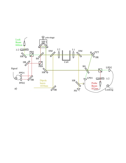
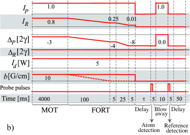
Figure 1: (color online). (a) Sketch of the setup of the interferometer with following elements: BS - 50/50 beam-splitter; PBS - polarizing beam-splitter; L1 & L2 - $f=100\leavevmode\nobreak\ \mathrm{mm}$ achromatic lenses; DM - dichroic mirrors (HT @ 852nm, HR @ 1030 nm); PZT - Piezo electric tube; PPD1 & -2 - Hamamatsu low noise, high gain photodiodes for probe detection; LPD1 & 2 - photodetectors for locking beam detection; and half wave plates $\lambda/2$. (b) Loading sequence of the dipole trap along with detection and reference pulse trains. The probe pulse duration and repetition rates are specified in the text for the different experiments

III Dipole trap characterization

III.1 Atomic sample preparation

The general loading sequence of the dipole trap is shown in Fig. 1(b). Initially, the atomic sample is prepared in a standard six beam Cs magneto-optical trap (MOT). The red detuning of the cooling laser is set to $-6\gamma$. The number of atoms collected in the MOT varies from $7.5\times 10^{7}$ to $10^{8}$ depending on the partial pressure of the Cs vapor. The typical density of the atoms in the MOT is $1.3\times 10^{9}$ atoms/cm³.

In the next step, the atoms are further sub-doppler cooled for 150 to 200 ms. During this stage the cooling laser detuning is reduced to $-8\gamma$ and simultaneously the intensity of the hyperfine repump light is reduced.

Finally, the cold Cs sample is transferred into a far-off-resonant optical dipole trap (FORT) created by a single light beam focused at the center of the MOT. The dipole trap laser beam is generated by an Yb:YAG laser at a wavelength of 1030 nm. The waist of the trapping beam is estimated to be 40 $\mu$m, which along with a power of 3.5 W amounts to a maximum optical potential depth of $U_{\mathrm{dip}}/k_{B}=\mathrm{\leavevmode\nobreak\ 380\leavevmode\nobreak\ \mu K}$. The typical density of atoms in the $F=4$ state is as high as 8$\times$10¹⁰ atoms/cm³, which is an increase of almost 62 times compared to the MOT density. The atoms are held in the FORT for variable times from 10 to 1000 ms before being detected with the interferometer.

III.2 Interferometer

The interferometer, as sketched in Fig. 1(a), is in a Mach-Zehnder configuration with free space propagating beams. Compared with our earlier setup, which employed single mode fibers Oblak et al. (2005), this interferometer has significantly lower light losses, but is more susceptible to acoustic and vibrational disturbances. The linearly polarized probe beam hits the interferometer input coupler and splits 50/50 into the reference and the probe arm. The beam in the probe arm is carefully aligned co-linearly with the dipole trapping beam, so that the position of the probe beam waist (20$\mu$m) overlaps with the atomic sample. The pathlength of the reference arm can be coarsely aligned using the mirrors mounted on a translation stage, so that the distances covered by the probe and reference beams, when they are overlapped on the output coupler, are roughly equal. We achieve a maximum fringe visibility of $\mathcal{V}=98\%$, which is limited by mode mismatching of the two interferometer arms. The pulsed probe beam is detected with a balanced detection schemeHansen et al. (2001) using the low noise photodiodes $PPD1$ and $PPD2$. From the integral of the differential photocurrent $i_{-}$ over the pulse duration, we extract the pulse area. The mean value gives the phase-shift, and the variance gives information about the phase fluctuations.

As in our previous work Oblak et al. (2005) the Mach-Zehnder interferometer is locked to the interference signal obtained from an auxiliary off-resonant CW laser. The locking beam propagates through the interferometer along the same paths as the probe beam but in the opposite direction and with orthogonal polarization. The wavelength and power of the locking laser are 860 nm and 1 mW, respectively. As discussed in Sec.II.2, to suppress the influence of amplitude and phase noise we lock the interferometer to half fringe at the white light position, corresponding to a nearly zero path length difference with the help of the procedure described in Oblak et al. (2005).

Having implemented all the measures for removing undesirable noise contributions, the fluctuations in our interferometer signal must be due only to the quantum noise of the probe light. As a measure of the instability or noise of the interferometer signal we use the two point variance $\sigma^{2}(\tau_{0})$ defined in Oblak et al. (2005), which describes the variation of the collected phase-shift from a sequence of light pulses with a certain duration $\tau$ and time separation $\tau_{0}$ . In the experiment we send a thousand probe pulses of 2$\mathrm{\mu s}$ duration with $T=6\leavevmode\nobreak\ \mathrm{\mu s}$ repetition period. Then the integrated pulse areas are used to compute the two point variance $\sigma^{2}(\tau_{0})$.

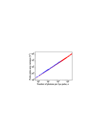
Figure 2: (color online). Noise in the amplitude $x$ ($\circ$) and phase $y$ ($\square$) quadratures of the probe light. Fits to the data in log-log scale give slopes of $1.036\pm 0.008$ (red) for the amplitude and $0.990\pm 0.005$ (blue) for the phase quadrature

The quantum shot noise of light will cause the two point variance to grow proportionally to the probe power. On the other hand, classical noise will result in a quadratic growth of $\sigma^{2}(\tau_{0})$ with the probe power. To verify the sensitivity of the balanced detection we detect the noise in the amplitude quadrature by splitting the light, from the reference arm only, onto the probe detectors. The fit to the data in Fig. 2 shows that amplitude noise scales linearly with the number of photons in the probe beam, indicating that our balanced detection is shot noise limited. The detectors remain shot noise limited on all time-scales relevant for the measurements.

Subsequently, we unblock the probe arm, whereby the detection becomes sensitive to phase fluctuations. The result in Fig. 2 shows that the two point variance scales linearly with the photon number. On this, we conclude that on the 6 $\mu$s time-scale the detector and interferometer sensitivities are limited only by quantum shot noise for the probe power range from 0.2$\mu$W - 13$\mu$W corresponding to around 2 million - 112 million photons per 2$\mu$s pulse. When the pulses have a larger temporal separation the interferometer does not remain shot-noise limited for high probe powers. In general the upper power at which the interferometer is shot noise limited decreases with increasing pulse separation. For measurement on the scale of several ms we find that a probe power of 150 nW ensures shot-noise limited operation and at same time fulfils the requirement that the detection be non-destructive.

As for the general feasibility of interferometric measurements it has been verified experimentally in a simplified setup  Figl et al. (2006) that through careful design the acoustic noise can be suppressed to below the shot noise level on minute long time-scales.

III.3 Interferometry with dipole trapped atoms

In this section we will present the results from the non-destructive characterization of a dipole trapped atomic sample. Probe light is provided by a grating stabilized laser diode and detuned by $100\mathrm{MHz}$ from the cycling $6S_{1/2}(F=4)\rightarrow 6S_{3/2}(F^{\prime}=5)$ transition in caesium. The probe power is either 150 or 300$\mathrm{nW}$. The measurements are done as follows: the dipole trap is loaded using the sequence described in Sec. III.1. After a variable storage time delay, but not shorter than 10 ms, the atoms in the dipole trap are probed by a train of light pulses with a typical pulse duration of 2 $\mu\mathrm{s}$ and a repetition period of 6 $\mu\mathrm{s}$ to 100 $\mu\mathrm{s}$, depending on the measurement. The number of pulses is chosen on the purpose of the measurement, but usually varies from 10 to 100. After probing the atoms, resonant light from the MOT cooling beams is applied in order to remove the atoms from the probing volume and consecutively a reference measurement is taken using the same probe light characteristics. The first measurement collects information about atomic sample, recorded in the light phase, and the second is a reference with no atoms in the probe arm that eliminates the slow drifts of the residual interferometer phase.

In the following we present the results of this measurement method applied to various dynamics of the FORT.

III.3.1 Loading and loss dynamics

Here we will apply our non-destructive measurement method to determine the loading and loss parameters of our dipole trapped atomic sample. A comprehensive analysis of the loading dynamics of a FORT is done by Kuppens et al. Kuppens et al. (2000). The dynamics of the loading process into the $F=4$ hyperfine ground state are described by the equation:

$$\frac{dN_{4}}{dt}=R_{0}\exp\left(-\gamma_{MOT}t\right)-\Gamma_{L}N_{4}-\beta_{L}N_{4}^{2},$$ (5)

where $\gamma_{MOT}$ is the rate at which the MOT loses atoms, $R_{0}$ is the loading rate of the dipole trap, $\Gamma_{L}$ is the light assisted loss rate of the FORT, $\beta_{L}$ is the light assisted density dependent loss rate of the FORT.

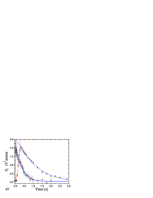
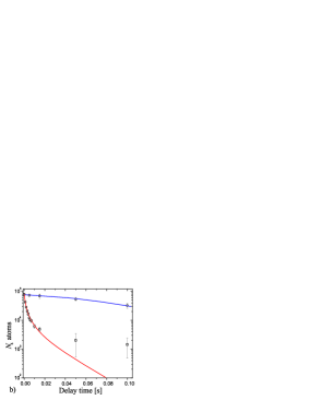
Figure 3: (color online). Loading and loss curves of FORT: (a) Number of atoms loaded in the FORT as a function of loading time for the compression ($\square$) and molasses ($\circ$) regimes. The curves are fits to different parts of Eg.(5). (b) Loss curves of FORT. With MOT light on (squares, red curve). Without any MOT light (circles, blue). (c) Light induced density dependent losses as function of light frequency. The line shows the two body loss level ”in the dark.”

When the loading is complete, the MOT trapping fields are switched off and only the FORT potential remains. The evolution of the FORT is now governed by the equation

$$\frac{dN_{4}}{dt}=-\Gamma N_{4}-\beta N_{4}^{2},$$ (6)

which contains the light-independent loss coefficients $\Gamma$ and $\beta$. The losses are a result of the natural decay of the dipole trap due to collisions with the background gas particles or with other caesium atoms, and are generally different from the coefficients $\Gamma_{L}$ and $\beta_{L}$, that reflect the impact of the MOT light.

For the experimental investigation of the loading of the FORT from the MOT we consider two regimes. In the first compression regime the magnetic field is gradually increased from $10\mathrm{G/cm}$ to $12\mathrm{G/cm}$ during the loading of the FORT, implying that the density of the MOT increases during the loading. At the end of the loading, the magnetic field is switched off rapidly on a timescale of $100\leavevmode\nobreak\ \mu$s Garrido Alzar et al. (2004). The detuning of the cooling light at the beginning of loading is $-\mathrm{6\gamma}$. In the second molasses regime the atoms are loaded in the FORT using optical molasses cooling. This means that the magnetic field is switched off gradually during the loading of the FORT (see dashed line in Fig. 1(b)). The detuning of MOT light is reduced to $-\mathrm{13\gamma}$.

	Comp	Mol	Light	No light
$\small{R_{0}}$	$1.34\times 10^{7}$	$3.2(6)\times 10^{4}$	-	-
$\gamma_{MOT}$	831	5	-	-
$\Gamma_{L}$	3.5	1.2	47(20)	-
$\beta_{L}$	$1.1\times 10^{-4}$	$3(1)\times 10^{-5}$	$1.1(1)\times 10^{-2}$	-
$\Gamma$	-	-	-	21(1)
$\beta$	-	-	-	$2.3(2)\times 10^{-4}$

Table 1: Loading and loss parameters of the dipole trap in $\mathrm{Hz}$

In order to determine the loading and loss rates we vary the duration of the loading stage and measure the number of atoms that are loaded into the FORT. The number of atoms as a function of the loading time for two loading schemes are presented in Fig. 3(a). The power of the probe beam is $0.3\leavevmode\nobreak\ \mu\mathrm{W}$ and the detuning is set to $\Delta_{\mathrm{45}}=\mathrm{100\leavevmode\nobreak\ MHz}$ with respect to the cycling $F=4\rightarrow F^{\prime}=5$ transition. The number of atoms is obtained from the mean phase-shift of a train of 10 pulses with $2\leavevmode\nobreak\ \mu\mathrm{s}$ duration and repetition period of $40\leavevmode\nobreak\ \mu\mathrm{s}$ for the case in Fig. 3(a) (squares) and $10\leavevmode\nobreak\ \mu\mathrm{s}$ in the case of Fig. 3(a)(circles). Each point in Fig. 3(a) represents an average of 20 experimental runs.

The general solution to Eq.(5) is expressed with Bessel functions, which makes it involved and time consuming to fit the experimental data on an ordinary PC. To circumvent this issue, we have adopted a method of separating the loading process to two parts: initial loading during which the FORT gains atoms from the MOT, and subsequently loss of atoms caused by collisions and decay due to cooling light. Thus, for short times we fit to a solution of the differential equation which includes only the first term on the right-hand-side of Eq. (5), and for longer times we fit to a solution of the Eq. (5) with only the last two terms.

The values for the loss coefficients obtained from the fits in Fig. 3(a) are compiled in Table 1. We see that in the compression regime loading is faster due to the magnetic field gradient, which keeps the MOT compressed, helping atoms to be transferred to the FORT. However, the density dependent loss-mechanism has a larger effect in compression regime compared to the less dense molasses regime where the $\beta_{L}$ coefficient is around 30 times lower. The difference in $\Gamma_{L}$ between the two regimes is not significant since it does not depend on the atomic density.

Although the above investigation provides a good characterization of the FORT loading, the actual values for the loss coefficients obtained are coupled to the sub-Doppler cooling used to lower the temperature of the atoms. Specifically, the detuning of the light is gradually increased during the loading. To study the light induced losses independently from the loading process we use the method suggested in Kuppens et al. (2000). After storing the atoms in the dipole-trap for 10 ms we switch the MOT beams back on with total intensity of the cooling laser of $4.6\leavevmode\nobreak\ \mathrm{mW/cm^{2}}$, detuning of $-16\gamma$, and repump laser intensity of $1.1\leavevmode\nobreak\ \mathrm{mW/cm^{2}}$ on resonance. The light is kept on for a varying duration and when it is switched off again the number of atoms remaining in the FORT is measured. Each point in Fig.3(b)(squares) represents an average value of the number of atoms probed with 10 pulses of $\mathrm{2\leavevmode\nobreak\ \mu s}$ duration and repetition period of $\mathrm{40\leavevmode\nobreak\ \mu s}$. The data is fitted to the solution of Eq.(6) [Fig.3(b), red curve] and the loss coefficient values obtained from the fit are listed in the third column of Table.1. For comparison the losses in the FORT without any MOT light are also measured and plotted in Fig.3(b), circles.

The data clearly shows that the FORT undergoes severe losses due to light assisted collisions, so that the density dependent losses will prevail over the losses due to background gas collisions. The density independent loss rate is little affected by the presence of the light. We perform the same measurements at a range of detunings to determine how it affects the light assisted losses. In Fig. 3(c) we plot the fitted $\beta_{L}$ coefficients as function of the light detuning. As expected we see that the light assisted losses increase as the detuning is reduced.

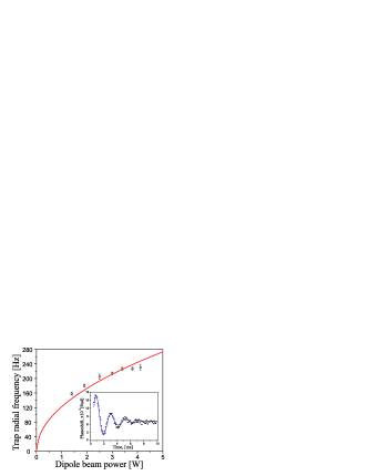
Figure 4: (color online). Trap radial oscillation frequency as function of dipole beam power. The estimated waist of dipole trap beam from this fit is $\mathrm{90(1)\mu m}$. The inset: Oscillation in the trap after its revival by switching the dipole trap laser again after 500 $\mu s$ release. The period of the damped oscillations corresponds to oscillation frequency of $453(3)\leavevmode\nobreak\ \mathrm{Hz}$.

III.3.2 Oscillation frequency

Here we adopt a different measurement technique and demonstrate that using the interferometric measurement we can extract information about important parameters of FORT in an measurement procedure which is significantly less time consuming than the conventional methods.

We induce radial oscillation in the FORT by switching the Yb:YAG trapping laser beam off for $\mathrm{500\leavevmode\nobreak\ \mu s}$ and subsequently turning it on again. The act of re-enforcing the trap potential when the cloud has started to expand will induce a ”breathing” oscillation of the radial size of the cloud of atoms, with a frequency that is twice the natural radial oscillation frequency of the trap. These oscillations are exponentially damped due to the anharmonicity of the confining potential. We track the radial ”breathing” mode of the cloud by sending a long pulse train of 100 pulses with $\mathrm{2\leavevmode\nobreak\ \mu s}$ duration, $\mathrm{100\leavevmode\nobreak\ \mu s}$ repetition period and power of $\mathrm{150\leavevmode\nobreak\ nW}$. The result of such a measurement is shown in the inset of Fig. 4. We emphasize that the measurement can be done in a single loading of the FORT and that the atomic sample is not destroyed by the measurement. All in all, the time needed for taking the data is at maximum $\mathrm{3min}$ in the case where we average over 50 cycles. We measured the breathing oscillations for several different values of the dipole beam power. The result is plotted in Fig. 4 and the fitted curve shows that the oscillation frequency follows the anticipated square-root dependence on beam power Boiron et al. (1998).

The oscillation frequency calculated from the initial estimate of the dipole-beam radius is 2.25 times larger than the measured value. We believe the discrepancy comes from the non-perfect spatial mode of our trapping laser, which can be inferred from the experimentally obtained value for the beam quality factor of $M^{2}=1.34$.

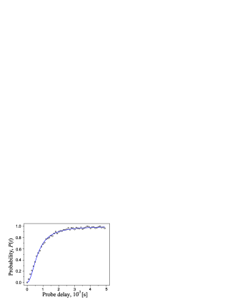
Figure 5: (color online). Ballistic expansion of the released atomic cloud probed in a single measurement by a train of 50 pulses, $\mathrm{100\mu s}$ apart, with probe power of $\mathrm{150\leavevmode\nobreak\ nW}$. The fit gives $\mathrm{T=15(2)\leavevmode\nobreak\ \mu K}$, and $\mathrm{\nu_{r}=275(4)\leavevmode\nobreak\ Hz}$ respectively for the temperature and radial oscillation frequency.

III.3.3 Temperature

Here we present our measurement of atom temperature using the interferometer phase-shift. After storage in the dipole trap the atoms are released by switching off the dipole laser, causing the atomic cloud to expand ballistically in a free fall. During the free expansion the cloud is probed by optical pulses and the measured atomic phase-shift is used to determine the fraction of atoms that have left the probe beam volume after a given time. In other words, we can measure the probability $P(t)$ of an atom initially inside the probe volume, to be outside it after a certain time. The probability $P(t)$ is found as a convolution of the ballistically expanding density profile and the probing Gaussian light beam. We construct a simple model that describes the evolution of $P(t)$ as a function of the expansion time and is similar to already known time-of-flight techniques Weiss et al. (1989). We derive an approximate expression for the probability function which has the following form:

$$P(t)=1-\frac{w_{0}^{2}+4\sigma_{r,0}^{2}}{w_{0}^{2}+4\sigma_{r}(t)^{2}}\exp\left\{-\frac{(gt^{2})^{2}}{2[w_{0}^{2}+4\sigma_{r}(t)^{2}]}\right\},$$ (7)

where $w_{0}=\mathrm{20\mu m}$ is the probe beam waist, $\sigma_{r}(t)=\sqrt{\sigma_{r,0}^{2}+\sigma_{v}^{2}t^{2}}$ is the time-dependent radius of atomic sample with $g$ the earth acceleration, $\sigma_{r,0}=\sqrt{k_{B}T/(M\omega_{r}^{2})}$ and $\sigma_{v}=\sqrt{k_{B}T/M}$ being the initial radial extension of the atomic cloud and the initial atom velocity respectively. Both $\sigma_{r,0}$ and $\sigma_{v}$ depend on the temperature $T$, Boltzman’s constant $k_{B}$, the trap radial angular frequency $\omega_{r}$, and $M$ the atomic mass of ${}^{133}\mathrm{Cs}$.

For the measurement the atoms are stored in the dipole trap for 50 ms before being released, after which probed by a pulse train with the first pulse arriving just after the atoms are released. The pulse train contains 50 pulses with a duration of $\mathrm{2\leavevmode\nobreak\ \mu s}$, repetition period of $\mathrm{100\leavevmode\nobreak\ \mu s}$, and optical power of $\mathrm{150\leavevmode\nobreak\ nW}$. The phase-shift of each pulse is normalized to the phase-shift of the first pulse and the fraction of atoms that have left the probing volume is calculated and plotted in Fig. 5. Hence, each point on the graph in Fig. 5 corresponds to a single pulse and the whole sequence of pulses belongs to a single measurement. Moreover, a single measurement trace represents a complete ballistic expansion of the cloud, free of shot-to-shot fluctuations in the atom number. To correct for any possible decay due to the probe light, we take a reference measurement with the dipole beam on and subtract it from the ballistic data. The estimated relative decay of the detected signal due to probe light depumping is found to be around $\mathrm{3.5\%}$.

The results obtained for the temperature are $\mathrm{T=15(2)\leavevmode\nobreak\ \mu K}$ and oscillation frequency $\mathrm{\nu_{r}=275(4)\leavevmode\nobreak\ Hz}$. The oscillation frequency is in a reasonable agreement with the previously obtained value of $\mathrm{244\leavevmode\nobreak\ Hz}$ (see Fig. 4) for a power of dipole laser of approximately $\mathrm{4\leavevmode\nobreak\ W}$.

As a comparison we explore a different measurement procedure, where the evolution of the phase-shift during the cloud expansion is compiled from several measurements done at various points of the expansion, similar to what would be the procedure for a destructive measurement. With this method we obtain a temperature estimate of $\mathrm{T=14.5(2)\leavevmode\nobreak\ \mu K}$, which agrees well with the above value. The radial oscillation frequency estimate of $\mathrm{\nu_{r}=259(4)\leavevmode\nobreak\ Hz}$ fits well with Fig. 4.

As a final verification of the results we directly measure the expansion of the cloud radius using fluorescence imaging on a CCD camera. By this means we get a value for the temperature of 14(2) $\mu$K, which agrees with the interferometric measurements to within 7 %

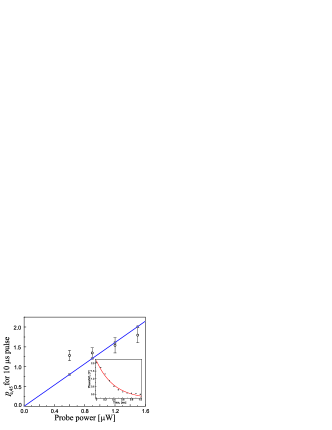
Figure 6: (color online). Pulse integrated rate of spontaneous emission. The experimentally obtained value for the $p_{e}$ parameter as a function of the probe power for a $\mathrm{10\leavevmode\nobreak\ \mu s}$ long probe pulses: values of $p_{e}$ for different power obtained from the fit of the phase-shift decay ($\circ$), theoretically calculated values for a probe beam waist radius of $\mathrm{21.2\leavevmode\nobreak\ \mu m}$ ($\square$), and a linear fit to the data (solid line). The inset shows the raw data for probe power of $\mathrm{1.2\leavevmode\nobreak\ \mu W}$.

III.4 Probability of real transitions

Here we want to verify the theoretical estimates of the destructiveness of the measurements due to absorption of probe light photons, which we in Sec. II.3 chose to gauge with the parameter $p_{e}$. The absorption of photons from the probe light comes as an inevitable side-effect of the dispersive measurement. Since the excitation is followed by spontaneous decay it will decohere the initial atomic state and on a longer time-scale de-pump the $F=4$ ground-level.

As the probe is blue detuned by 100 MHz from the $\mathrm{6S_{1/2}(F=4)\rightarrow 6P_{3/2}(F^{\prime}=5)}$ cycling transition, most excitations will populate the $F^{\prime}=5$ excited level from which atoms can only decay back to the $F=4$ ground level. The experimental method for estimating $p_{e}$, however, relies on the small chance of exciting atoms to the $\mathrm{F^{\prime}=4}$ excited state whereupon the atoms may decay to either the $F=3$ or $F=4$ ground levels. Hence, the excitation to the $F^{\prime}=4$ level will cause a reduction of population in the $F=4$ ground state that we can observe as a reduction of the phase-shift. Since the depumping parameter is proportional to the number of photons, we monitor the decay of the interferometer phase-shift as a function of the probe power. The direct experimental parameter is the characteristic time constant of the decay that we expect to decrease linearly with increasing probe power.

In the experiment we send a long pulse train consisting of 40 pulses of $\mathrm{10\leavevmode\nobreak\ \mu s}$ duration and $\mathrm{100\leavevmode\nobreak\ \mu s}$ repetition period through the atomic sample along with a reference pulse train. Each pulse in the train causes a small amount of depumping, which causes a smaller phase-shift of the subsequent pulse in the train. An example of a measurement trace for a probe power of $\mathrm{1.2\leavevmode\nobreak\ \mu W}$ is shown in the inset of Fig. 6. Altogether, the measurement is done at four different power levels of the 100 MHz blue-detuned probe beam.

The decay is modeled by a set of rate equations that take into account the two ground levels, the $F^{\prime}=4$ and $F^{\prime}=5$ excited levels and two optical fields, namely the probe and residual hyperfine re-pump fields. For a given probe power the value of $p_{e}$ is obtained by fitting the decay of the phase-shift to the expression obtained from the rate equations. The values of the depumping parameter are plotted against the probe power and fitted to a straight line as shown in Fig. 6. We can theoretically calculate $p_{e}$ using Eq.(3) and Eq.(4) and if we use a probe waist radius of $\mathrm{21.2\leavevmode\nobreak\ \mu m}$ the theoretical estimates coincide with the experimental fit. We see that for very low probe powers the pulse integrated probability of spontaneous emission per atom is less than one. The lowest power used in our characterization measurements is $\mathrm{150\leavevmode\nobreak\ nW}$ for a pulse duration of $\mathrm{2\leavevmode\nobreak\ \mu s}$. This would mean that the lowest photon scattering probability per atom is of the order of $p_{e}=0.038$.

IV Conclusion

In this paper we have demonstrated a novel method for non-destructive characterization of dipole trapped atomic sample using a shot-noise limited free-space white-light Mach-Zehnder interferometer.

The radial oscillation frequencies and temperature measurements were done in a single loading run, thus enabling us for fast characterization of atomic sample. The temperature measurement in both single and multiple runs agrees with the one obtained by fluorescence detection using a CCD camera. Furthermore, an estimation of the non-destructive character of the measurement has shown a pulse integrated probability of real transition for an atom to be as low as 0.038.

The real time monitoring of the phase-shift in a Mach-Zehnder interferometer allows for fast and non-destructive characterization of atomic samples. The method is applied to a dipole trapped atomic sample but with the same success it can be expanded to Bose-Einstein condensates, where the optical density is much higher and the absorption imaging does not give the necessary contrast Andrews et al. (1996). Moreover, our pulsed detection scheme allows for microsecond timescale monitoring of processes and phenomena taking place in an atomic cloud with a few thousand atoms, which in other cases as absorption or fluorescence imaging are not visible due to the limited measurement bandwidth.