Multiplexed Memory-Insensitive Quantum Repeaters

Abstract

Long-distance quantum communication via distant pairs of entangled quantum bits (qubits) is the first step towards more secure message transmission and distributed quantum computing. To date, the most promising proposals require quantum repeaters to mitigate the exponential decrease in communication rate due to optical fiber losses. However, these are exquisitely sensitive to the lifetimes of their memory elements. We propose a multiplexing of quantum nodes that should enable the construction of quantum networks that are largely insensitive to the coherence times of the quantum memory elements.

Quantum communication, networking, and computation schemes utilize entanglement as their essential resource. This entanglement enables phenomena such as quantum teleportation and perfectly secure quantum communication bb84 . The generation of entangled states, and the distance over which we may physically separate them, determines the range of quantum communication devices. To overcome the exponential decay in signal fidelity over the communication length, Briegel et al. briegel proposed an architecture for noise-tolerant quantum repeaters, using an entanglement connection and purification scheme to extend the overall entanglement length using several pairs of quantum memory elements, each previously entangled over a shorter fundamental segment length. A promising approach utilizes atomic ensembles, optical fibers and single photon detectors duan ; matsukevich ; chaneliere .

The difficulty in implementing a quantum repeater is connected to short atomic memory coherence times and large optical transmission loss rates. In this Letter we propose a new entanglement generation and connection architecture using a real-time reconfiguration of multiplexed quantum nodes, which improves communication rates dramatically for short memory times.

A generic quantum repeater consisting of $2^{N}+1$ distinct nodes is shown in Fig. 1a. The first step generates entanglement between adjacent memory elements in successive nodes with probability $P_{0}$. An entanglement connection process then extends the entanglement lengths from $L_{0}$ to $2L_{0}$, using either a parallelized (Fig. 1b), or multiplexed (Fig. 1c) architecture. This entanglement connection succeeds with probability $P_{1}$, followed by subsequent entanglement-length doublings with probabilities $P_{2}$,…,$P_{N}$, until the terminal quantum memory elements, separated by $L={2^{N}}L_{0}$, are entangled.

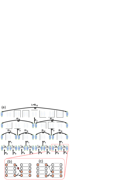
Figure 1: (a) Processes of an $N=3$ multiplexed quantum repeater. In addition to two terminal nodes the network has seven internal nodes consisting of two quantum memory sites containing $n$ independent memory elements. Entanglement generation proceeds with probability $P_{0}$, creating 8 entanglement lengths of $L_{0}$. In the lowest panel, shaded memory sites indicate successfully entangled segments. The $N=1$ level entanglement connection proceeds with probability $P_{1}$, producing four entangled segments of length $2L_{0}$. Nodes reset to their vacuum states by the connection are blank. The $N=2$ and $N=3$ levels proceed with probabilities $P_{2}$ and $P_{3}$. Each stage results in entanglement-length doubling, until an $N=3$ success entangles the terminal nodes. (b) and (c) show the topology of the $n$ memory element sets. The parallel architecture (b) connects entanglement only between memory elements with the same address. In contrast, multiplexing (c) uses a fast sequential scanning of all memory element addresses to connect any available memory elements.

For the simplest case of entanglement-length doubling with a single memory element per site ($N=n=1$), we calculate the average time to successful entanglement connection for both ideal (infinite) and finite quantum memory lifetimes. This basic process is fundamental to the more complex $N$-level quantum repeaters as an $N$-level quantum repeater is the entanglement-length doubling of two $(N-1)$-level systems.

Entanglement-length doubling with ideal memory elements.— Define a random variable $Z$ as the waiting time for an entanglement connection attempt (all times are measured in units of $L_{0}/c$, where the speed of light $c$ includes any material refractive index). Let $Y\equiv 1$ if entanglement connection succeeds and zero otherwise. Entanglement generation attempts take one time unit. The time to success is the sum of the waiting time between connection attempts and the 1 time unit of classical information transfer during each connection attempt,

$$T =(Z_{1}+1)Y_{1}+(Z_{1}+Z_{2}+2)(1-Y_{1})Y_{2}+$$ (1)

$$(Z_{1}+Z_{2}+Z_{3}+3)(1-Y_{1})(1-Y_{2})Y_{3}+...,$$

as Z,Y are independent random variables, it follows that

$$\langle T\rangle=\frac{\langle Z\rangle+1}{P_{1}},$$ (2)

In the infinite memory time limit, $Z$ is simply the waiting time until entanglement is present in both segments, i.e., $Z=\max\{A,B\}$, where $A$ and $B$ are random variables representing the entanglement generation waiting times in the left and right segments. As each trial is independent from prior trials, $A$ and $B$ are geometrically distributed with success probability $P_{0}$. The mean of a geometric random variable with success probability $p$ is $1/p$, and the minimum of $j$ identical geometric random variables is itself geometric with success probability $1-(1-p)^{j}$. From these properties it follows that,

$$\langle T\rangle_{\infty}=\frac{3-P_{0}^{2}}{P_{0}P_{1}(2-P_{0})}.$$ (3)

Entanglement-length doubling with finite memory elements.— For finite quantum memory elements Eqs. (1) and (2) still hold, but $Z$ is no longer simply $\max\{A,B\}$. Rather it is the time until both segments are entangled within $\tau$ time units of each other, where $\tau$ is the memory lifetime. For simplicity, we assume entanglement is unaffected for $\tau$, and destroyed thereafter. A new r.v. $M\equiv 1$ if $|A-B|<\tau$, zero otherwise. Due to the memoryless nature of the geometric distribution,

$$Z = \max\{A_{1},B_{1}\}M_{1}+\left(\min\{A_{1},B_{1}\}+\tau\right.$$ (4)

$$+ \max\{A_{2},B_{2}\})(1-M_{1})M_{2}+...$$

From this and Eq. (2) it follows that note

$$\langle Z\rangle_{\tau} =\frac{1}{P_{0}(2-P_{0}-2q_{0}^{\tau+1})}+\frac{2\tau q_{0}^{\tau+1}}{2-P_{0}-2q_{0}^{\tau+1}}$$ (5)

$$+\frac{2q_{0}(1-q_{0}^{\tau}(1+\tau P_{0}))}{P_{0}(2-P_{0}-2q_{0}^{\tau+1})},$$

$$\langle T\rangle_{\tau} =\frac{\langle T\rangle_{\infty}-(\frac{1+P_{0}}{P_{0}P_{1}})\frac{q_{0}^{\tau+1}}{1-P_{0}/2}}{1-\frac{q_{0}^{\tau+1}}{1-P_{0}/2}},$$

where $q_{0}\equiv 1-P_{0}$. Typically $P_{0}$ is small compared to $P_{1}$ as the former includes transmission losses. The terms in $\langle Z\rangle_{\tau}$ are, respectively, the time spent(I)waiting for entanglement in either segment starting from unexcited nodes,(II) fruitlessly attempting entanglement generation until the quantum memory in the first segment expires,(III) on successful entanglement generation in the other segment. When $P_{0}\ll 1/(\tau+1)$, memory times are much smaller than the entanglement generation time, and $\langle Z\rangle_{\tau}\approx 1/[P_{0}^{2}(1+2\tau)]+2\tau/[P_{0}(1+2\tau)]+2\tau^{2}(1-P_{0})/(1+2\tau)$, and term (I) dominates the entanglement-length doubling time. Fig. 2 shows the sharp increase in $\langle T\rangle_{\tau}$ for small $\tau$ characteristic of term (I).

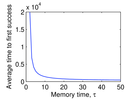
Figure 2: Plot of $\langle T\rangle_{\tau}$ against $\tau$. $P_{0}=0.01$, $P_{1}=0.5$. The minimum possible success time of 2 imposes a similar minimum of the on quantum memory element lifetimes.

Parallelization and multiplexing.— Long memory coherence times remain an outstanding technical challenge, motivating the exploration of approaches that mitigate the poor low-memory scaling. One strategy is to engineer a system that compensates for low success rates by increasing the number of trials, replacing single memory elements with $n>1$ element arrays. In a parallel scheme, the $i^{th}$ memory element pair in one node interacts only with the $i^{th}$ pair in other nodes, Fig.1b. Thus, a parallel repeater with $n2^{N+1}$ memory elements acts as $n$ independent $2^{N+1}$-element repeaters and connects entanglement $n$ times faster. A better approach is to dynamically reconfigure the connections between nodes, using information about entanglement successes to determine which nodes to connect. In this multiplexed scheme the increased number of node states that allow entanglement connection, compared to parallelizing, improves the entanglement connection rate between the terminal nodes.

We now calculate the entanglement connection rate $f_{\tau}$ of an $N=1$ multiplexed system. Unlike the parallel scheme, however, the entanglement connection rate is no longer simply $1/\langle T\rangle_{\tau}$. When one segment has more entangled pairs than its partner, connection attempts do not reset the repeater to its vacuum state and there is residual entanglement. Simultaneous successes and residual entanglement produce average times between successes smaller than $\langle T\rangle_{\tau}$. We approximate the resulting repeater rates when residual entanglement is significantly more probable than simultaneous successes. This is certainly the case in both the low memory time limit and whenever $nP_{0}\ll 1$. Our approximation modifies Eq. (4) by including cases where the waiting time is zero due to residual entanglement. In $Z$ of Eq.(4), the $\min\{A_{i},B_{i}\}$ terms represent the waiting time to an entanglement generation success starting from the vacuum state. Multiplexing modifies Eq.(4) in the following way: for each $i=1,..\infty$ we replace $(A_{i},B_{i})$ $\rightarrow$ $(\min\{A_{i,j}\},\min\{B_{i,k}\})$, where $j$ and $k=1,...,n$. The effect of the residual entanglement is approximated by the factor $\alpha$: $\min\{A_{i},B_{i}\}\rightarrow\alpha\min\{\min\{A_{i,j}\},\min\{B_{i,k}\}\}$, where 1-$\alpha$ is the probability of residual entanglement. Eq. (4) now approximates the average time between successes. Using Eqs. (2), (4) and the distributions of $\min\{A_{i,j}\}$ and $\min\{B_{i,k}\}$, the resulting rate is

$$\langle f\rangle_{\tau,n} =\frac{P_{1}(1-q_{0}^{n})(1+q_{0}^{n}-2q_{0}^{n(\tau+1)})}{1+2q_{0}^{n}-q_{0}^{2n}-4q_{0}^{n(\tau+1)}+2q_{0}^{n(\tau+2)}+\alpha},$$

$$\alpha ={\frac{q_{0}^{n-1}(1-q_{0}^{n})(1-q_{0}^{2n-1}+2q_{0}^{3n-2}(1-q_{0}^{\tau(2n-1}))}{(1-q_{0}^{2n-1})(1+q_{0}^{n}-2q_{0}^{(\tau+1)n})}}.$$

When $n=1$, $\alpha=1$, as required. Further, as $nP_{0},\tau$ become large, $\alpha\rightarrow 0$ showing the expected breakdown of the approximation. As $n\rightarrow\infty$, $\alpha$ should approach $1/2$.

Fig. 3(a) demonstrates that, as expected, multiplexed connection rates exceed those of parallelized repeaters. The improvement from multiplexing in the infinite memory case is comparatively modest. However, the multiplexed connection rates are dramatically less sensitive to decreasing memory lifetimes. Note that the performance of multiplexing $n=5$ exceeds that parallelizing $n=10$, reflecting a fundamental difference in their dynamics and scaling behavior. Fig. 3(b) further illustrates the memory insensitivity of multiplexed repeaters by displaying the fractional rate $f_{\tau}/f_{\infty}$. As parallelized rates scale by the factor $n$, such repeaters all follow the same curve for any $n$. By contrast, multiplexed repeaters become less sensitive to coherence times as $n$ increases. This improved performance in the low memory limit is a characteristic feature of the multiplexed architecture.

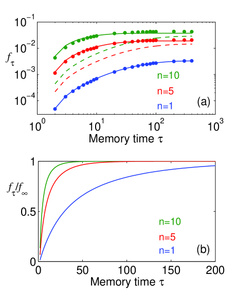
Figure 3: Comparison of entanglement connection rate $f_{\tau}$ for parallel (dashed) and multiplexed (solid) architectures as a function of coherence time. $P_{0}=0.01$, $P_{1}=0.1$. (a) Solid circles denote simulated values for the multiplexed case. (b) Parallel repeaters of any $n$ value follow the $n=1$ line. As $n$ increases, multiplexed scaling improves while parallel scaling remains constant.

$N$-level quantum repeaters.— For $N>1$ repeaters we proceed by direct computer simulation, requiring a specific choice of entanglement connection probabilities. We choose the implementation proposed by Duan, Lukin, Cirac, and Zoller (DLCZ) duan . The DLCZ protocol requires a total distance $L$, the number of segments $2^{N}$, the loss $\gamma$ of the fiber connection channels, and the efficiency $\eta$ of retrieving and detecting an excitation created in the quantum memory elements.

Let $P_{0}=\eta_{0}\exp(-{\gamma L_{0}}/2)$, where $\eta_{0}$ is related to the fidelity $F\approx 2^{N}(1-\eta_{0})$ duan . Recursion relations give the connection probabilities: $P_{i}=({\eta}/(c_{i-1}+1))(1-{\eta}/({2\beta(c_{i-1}+1)}))$, $c_{i}\equiv 2c_{i-1}+1-\eta/\beta$, $i=1,...N$. Neglecting detector dark counts, $c_{0}=0$. For photon number resolving detectors $\beta=1$ (PNRDs) duan . $\beta=2$ for non-photon resolving detectors (NPRDs). For values of $\eta<1$ photon losses result in a vacuum component of the connected state in either case. For NPRDs, the indistinguishability of one- and two-photon pulses requires a final projective measurement, which succeeds with probability $\epsilon=1/(c_{3}+1)$, see Ref. duan for a detailed discussion.

Consider a 1000 km communication link. Assume a fiber loss of $10\gamma/\ln 10=0.16$ dB/km, $\eta_{0}=0.01$, and $\eta=0.9$. Taking $N=3$ ($L_{0}=125$ km) gives $P_{0}=0.001$. For concreteness we treat the NPRD case, producing connection probabilities: $P_{1}=0.698$, $P_{2}=0.496$, $P_{3}=0.311$, and $\epsilon=0.206$. Fig. 3 demonstrates agreement with the exact predictions for $n=1$ and the approximate predictions for $n>1$. The slight discrepancies for long memory times with larger $n$ are uniform and understood from the simultaneous connection successes neglected in Eq. (6).

An $N$-level quantum repeater succeeds in entanglement distribution when it entangles the terminal nodes with each other. Fig. 4 shows the entanglement distribution rate of a 1000 km $N=3$ quantum repeater as a function of the quantum memory lifetime. Remarkably, for multiplexing with $n\gtrsim 10$ the rate is essentially constant for coherence times over 100 ms, while for the parallel systems it decreases by two orders of magnitude. For memory coherence times of less than 250 ms, one achieves higher entanglement distribution rates by multiplexing ten memory element pairs per segment than parallelizing 1000. In the extreme limit of minimally-sufficient memory coherence times set by the light-travel time between nodes, each step must succeed the first time. The probabilities of entanglement distribution scale as $nP_{0}^{2^{N}}$ (parallelized) and $(nP_{0})^{2^{N}}$ (multiplexed), for $nP_{0}\ll 1$.

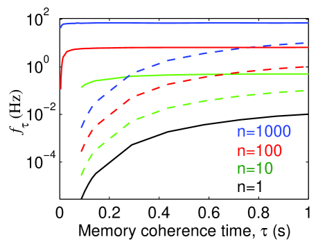
Figure 4: Simulated entanglement distribution over $1000$ km for multiplexed (solid) and parallel (dashed) $N=3$ quantum repeaters. For $\tau\geq 100$ msec, the multiplexed distribution rate is almost flat for $n\gtrsim 10$; parallel rates decrease by two orders of magnitude. For low memories a multiplexed $n=10$ repeater outperforms an $n=1000$ parallelization.

Communication and cryptography rates.— The DLCZ protocol requires two separate entanglement distributions and two local measurements to communicate a single quantum bit. The entanglement coincidence requirement and finite efficiency qubit measurements result in communication rates less than $f_{\tau}$. Error correction/purification protocols, via linear-optics-based techniques, will further reduce the rate and may require somewhat lower values of $\eta_{0}$ than the one used in Fig. 4, to maintain sufficiently high fidelity of the final entangled qubit pair duan ; bennett1 . We emphasize that it is the greatly enhanced entanglement distribution rates with multiplexing that make implementation of such techniques feasible.

Multiplexing with atomic ensembles.— A multiplexed quantum repeater could be implemented using cold atomic ensembles as the quantum memory elements, subdividing the atomic gas into $n$ independent, individually addressable memory elements, Fig. 1c. Dynamic addressing can be achieved by fast (sub-microsecond), two-dimensional scanning using acousto-optic modulators, coupling each memory element to the same single-mode optical fiber. Consider a cold atomic sample 400 $\mu$m in cross-section in a far-detuned optical lattice. If the addressing beams have waists of 20 $\mu$m, a multiplexing of $n>100$ is feasible. To date, the longest single photon storage time is 30 $\mu$s, limited by Zeeman energy shifts of the unpolarized, unconfined atomic ensemble in the residual magnetic field dspg . Using magnetically-insensitive atomic clock transitions in an optically confined sample, it should be possible to extend the storage time to tens of milliseconds, which should be sufficient for multiplexed quantum communication over 1000 km.

Summary.— Multiplexing offers only marginal advantage over parallel operation in the long memory time limit. In the opposite, minimal memory limit, multiplexing is $n^{2^{N}-1}$ times faster, yet the rates are practically useless. Crucially, in the intermediate memory time regime multiplexing produces useful rates when parallelization cannot. As a consequence, multiplexing translates each incremental advance in storage times into significant extensions in the range of quantum communication devices. The improved scaling outperforms massive parallelization with ideal detectors, independent of the entanglement generation and connection protocol used. Ion-, atom-, and quantum dot-based systems should all benefit from multiplexing.

We are particularly grateful to T. P. Hill for advice on statistical methods. We thank T. Chanelière and D. N. Matsukevich for discussions and C. Simon for a communication. This work was supported by NSF, ONR, NASA, Alfred P. Sloan and Cullen-Peck Foundations.

References

- (1) C. H. Bennett and G. Brassard, in Proceedings of the International Conference on Computers, Systems and Signal Processing 175 (IEEE, New York, 1984); C. H. Bennett et al., Phys. Rev. Lett. 70, 1895 (1993); A. K. Ekert, Phys. Rev. Lett. 67, 661 (1991); D. Bouwmeester et al., Nature (London) 390, 575 (1997); E. Knill, R. Laflamme, and G. J. Milburn, Nature (London) 409, 46 (2001).
- (2) H. J. Briegel, W. Duer, J. I. Cirac, and P. Zoller, Phys. Rev. Lett. 81, 5932 (1998); W. Duer, H. J. Briegel, J. I. Cirac, and P. Zoller, Phys. Rev. A 59, 169(1999).
- (3) L.-M. Duan, M. Lukin, J. I. Cirac, and P. Zoller, Nature (London) 414, 413 (2001).
- (4) D. N. Matsukevich and A. Kuzmich, Science 306, 663 (2004); D. N. Matsukevich et al., Phys. Rev. Lett. 95, 040405 (2005); D. N. Matsukevich et al., Phys. Rev. Lett. 96, 030405 (2006).
- (5) T. Chanelière et al., Phys. Rev. Lett. 96, 093604 (2006).
- (6) Note that is independent from , but not from , since . The calculation of is simplified by using . Furthermore, as is either 0 or 1, is equal to the probability that .
- (7) C. H. Bennett et al., Phys. Rev. Lett. 76, 722 (1996); S. Bose, V. Vedral, and P. L. Knight, Phys. Rev. A 60, 194 (1999); J.-W. Pan et al., Nature (London) 410, 1067 (2001); T. Yamamoto et al., Nature (London) 423, 343 (2003).
- (8) D. N. Matsukevich et al., Phys. Rev. Lett. 97, 013601 (2006).