Implementation of controlled SWAP gates for quantum fingerprinting and photonic quantum computation

Abstract

We propose a scheme to implement quantum controlled SWAP gates by directing single-photon pulses to a two-sided cavity with a single trapped atom. The resultant gates can be used to realize quantum fingerprinting and universal photonic quantum computation. The performance of the scheme is characterized under realistic experimental noise with the requirements well within the reach of the current technology.

PACS numbers: 03.67.-a, 42.50.Gy, 42.50.-p

Several quantum cryptographic schemes, such as quantum fingerprinting 1 and quantum digital signatures 2 , require the controlled SWAP (CSWAP) gates as the critical element for their realization. The qubits in these schemes are carried by photon pulses as photons are the only viable choice for remote quantum communication. The essential requirement for implementation of these schemes is to measure the overlap of two $n$-qubit wave functions $\left|\Psi\right\rangle$ and $\left|\Psi^{\prime}\right\rangle$. A multi-qubit CSWAP gate provides the simplest method for realization of this measurement 1 ; 2 . For a CSWAP gate, conditioned on the state $\left|1\right\rangle_{c}$ of the control qubit $c$, the two sets of target qubits $A=\{1,2,\cdots,n\}$ and $B=\{1^{\prime},2^{\prime},\cdots,n^{\prime}\}$ exchange their quantum states, so in general, we have

$$U_{\text{CSWAP}}\left(c_{0}\left|0\right\rangle_{c}+c_{1}\left|1\right\rangle_{c}\right)\otimes\left|\Psi\right\rangle_{A}\otimes\left|\Psi^{\prime}\right\rangle_{B}$$ (1)

$$= c_{0}\left|0\right\rangle_{c}\otimes\left|\Psi\right\rangle_{A}\otimes\left|\Psi^{\prime}\right\rangle_{B}+c_{1}\left|1\right\rangle_{c}\otimes\left|\Psi^{\prime}\right\rangle_{A}\otimes\left|\Psi\right\rangle_{B}.$$

If the control qubit is initially prepared in the state $\left(\left|0\right\rangle_{c}+\left|1\right\rangle_{c}\right)/\sqrt{2}$, and then measured in the basis $\left\{\left|\pm\right\rangle_{c}\equiv\left(\left|0\right\rangle_{c}\pm\left|1\right\rangle_{c}\right)/\sqrt{2}\right\}$ after the CSWAP gate, the probability to get the outcome “$-$” is given by $p_{-}=1-\left|\langle\Psi|\Psi^{\prime}\rangle\right|^{2}$, which shows exactly the information about the state overlap $\left|\left\langle\Psi|\Psi^{\prime}\right\rangle\right|$. So the central problem for implementation of these cryptographic schemes becomes how to realize a multi-qubit CSWAP gate.

In this paper, we propose a scheme to realize a multi-qubit CSWAP gate on two sequences of photon pulses $1,2,\cdots,n$ and $1^{\prime},2^{\prime},\cdots,n^{\prime}$ by simply transferring them through a single atom cavity. The cavity is two-sided, and the pulse sequences are incident from the different side mirrors. The atom inside the cavity plays the role of the control qubit. Under an appropriate atomic level configuration, this setup realizes exactly the CSWAP gate on the two pulse sequences. Beyond its applications for implementation of the above quantum cryptographic protocols, we also show that a simple version of this CSWAP gate, together with single-bit polarization rotations, realize universal quantum computation with photon pulses as qubits. Compared with the recent proposal of the photonic computation scheme based on the single-sided cavities 3 , this scheme has the advantage that it is directly built on the state-of-the-art two-sided cavities 4 . The same scheme also applies to other experimental setups with optical resonators, such as a quantum dot inside a solid state cavity 5 ; 6 ; 7 . To characterize performance of the CSWAP gate under influence of realistic experimental noise, we provide detailed theoretical modeling, and the calculation shows the practicality of the gate under typical configurations of either the atomic or the solid-state cavities. In particular, the scheme requires neither the good cavity limit nor the Lamb-Dicke condition for the trapped atom, which significantly simplifies its experimental realization.

First, we explain the basic idea of our scheme for implementation of the multi-qubit CSWAP gate. Consider an atom trapped in a two-sided optical cavity with the relevant atomic levels shown in Fig.1. The cavity supports two eigenmodes $a_{h}$ and $a_{v}$ with different polarizations (horizontal “$h$” and vertical “$v$”, respectively). These two modes are resonantly coupled to the corresponding atomic transitions $|0\rangle\leftrightarrow|e_{h}\rangle$ and $|0\rangle\leftrightarrow|e_{v}\rangle$ ($|e_{h}\rangle$ and $|e_{v}\rangle$ could be superpositions of the Zeeman states on the same excited hyperfine manifold). The state $|1\rangle$ is on a different hyperfine level in the ground-state manifold, and is decoupled from the cavity modes due to the large hyperfine splitting. The two cavity modes $a_{h}$ and $a_{v}$ are resonantly driven by the “$h$” and “$v$” polarization components of the single-photon pulses incident on the cavity mirrors, respectively. Each single-photon pulse represents an optical qubit, with its qubit basis-state carried by the polarization “$h$” or “$v$”.

If the atom is prepared in the state $|1\rangle$, the input pulses basically see an empty cavity as the atom is decoupled from the cavity modes. With such a resonant cavity, the input pulses from both sides will directly go through if their bandwidth is significantly smaller than the cavity decay rate $\kappa$ (assuming that both mirrors of the cavity give rise to the same decay rate). The states of the two pulse sequences from different sides are exchanged. (See Fig.1 for convention of the notation. We assume that the pulses from different sides have the same pulse shape.) However, if the atom is prepared in the state $|0\rangle$, due to the strong atom-cavity coupling, the transmission spectrum of the dressed cavity is significantly modified, and the pulses from both sides will be reflected by the cavity mirrors if their bandwidth is significantly smaller than $g^{2}/\kappa$, where $g$ is the atom-cavity coupling rate (see the following theoretical modeling). The states of the pulses remain unchanged note1 . From consideration of the above two cases, we see that if the atom is prepared in a superposition of the states $|0\rangle$ and $|1\rangle$, this cavity setup performs exactly the CSWAP gate described by Eq. (1), with the atom as the control qubit and the two $n$-qubit pulse-sequences on different side mirrors as the target qubits.

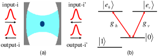
Figure 1: (a) Schematic setup for implementation of the multi-qubit CSWAP gate. Two pulse sequences $i,(i=1,2\cdots n)$ and $i^{\prime},(i^{\prime}=1^{\prime},2^{\prime}\cdots n^{\prime})$ are incident on and then reflected from (or transmitted through) the single-atom cavity. (b) Configuration of the relevant atomic levels.

As mentioned before, the multi-qubit CSWAP gate implemented by this cavity setup is ideal for the measurement of overlap of two $n$-qubit wave functions carried by the photon pulses. Therefore, the scheme is critical for realization of a number of quantum cryptographic protocols, including quantum fingerprinting and quantum digital signature 1 ; 2 . Beyond this important application, here we also want to show that the simplest version of this gate, the CSWAP on two optical qubits (denoted as CSWAP₂), also provides a critical gate, which, together with simple single-qubit rotations, realize universal quantum computation. In this computational scheme, the qubits are represented by the single-photon pulses, which have the advantages of being relatively easy to scale to many qubits and to integrate into quantum networks. The atom (or the quantum dot in the solid-state cavity) only acts as an ancilla qubit which mediates strong interaction between the photons during the gate operation.

To see the universality of the CSWAP₂ gate, it is enough to show that, together with single-bit rotations, it leads to the standard controlled phase flip (CPF) gate on two arbitrary photonic qubits. In Fig. 2(a), from the CSWAP₂ gates we give one construction of the CPF gate $U_{CPF}=e^{i\pi|hv\rangle_{12}\left\langle hv\right|}$, which flips the phase of the photons 1 and 2 if and only if they are in the state component $|hv\rangle$. The atomic qubit is initially prepared in the state $|\varphi\rangle_{a}=(|0\rangle+|1\rangle)/\sqrt{2}$, which is recovered after the whole operation. In this construction, we use four CSWAP₂ gates, together with a few single-bit Hadamard gates H and $i$-phase gates (the latter adds a phase $i$ to the state component $|1\rangle$). This construction can be further simplified if we use feed-forward from a measurement on the atomic qubit. In Fig. 2b, we give a simplified circuit which uses only two CSWAP₂ gates. After the operation represented by the left side of this circuit, we perform a measurement on the atomic qubit in the basis $\left\{|0\rangle,|1\rangle\right\}$, and upon the outcome “$1$”, we add a $\sigma_{z}=|h\rangle\langle h|-|v\rangle\langle v|$ ($Z$-gate) to each of the photonic qubits. One can verify that the whole operation also performs the gate $U_{CPF}$ on the two photonic qubits. These constructions prove that the CSWAP₂ gates, combined with single-bit rotations, indeed realize universal quantum computation on photon pulses.

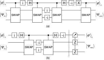
Figure 2: (a)A circuit to construct a controlled phase flip gate from the CSWAP gates. (b)An alternative circuit which uses only two CSWAP gates, but with feed-forward of a measurement on the atomic qubit (the right side of the dashed line, see the text for explanation).

Now we proceed to present the detailed theoretical modeling of interaction between photonic pulses and an atom inside a two-sided cavity. This calculation serves for two purposes; first, we need to prove the statements made before for the principle of the CSWAP gate. In particular, we will show that the pulse will have reflection or transmission conditional on the atomic state if its bandwidth is much smaller than the coupling rates $\kappa$ and $g^{2}/\kappa$. Second, we also want to characterize the influence of noise on this gate scheme. The most important noise here is the intrinsic atomic spontaneous emission, which causes loss of photons to uncontrolled directions. There could be other source of noise, such as the light absorption/scattering at the cavity mirrors. The effect of the latter, however, is very similar to the atomic spontaneous emission and thus can be similarly modeled.

The interaction between the atom (or, in general, the dipole) and the cavity modes is described by the Hamiltonian in the rotating frame (see Fig. 1 for the notations)

$$H=\sum_{\mu=h,v}g_{\mu}\left(\sigma_{\mu}^{+}a_{\mu}+\sigma_{\mu}^{-}a_{\mu}^{\dagger}\right),$$ (2)

where $\sigma_{\mu}^{+}\equiv|e_{\mu}\rangle\langle 0|$ is the atomic raising operator, $\mu=h,v$ denote the polarization modes, and $g_{{}_{\mu}}$ are the corresponding atom-cavity coupling rates. The cavity modes $a_{\mu}$ are driven by the corresponding input fields $a_{\mu,l}^{in}$ and $a_{\mu,r}^{in}$ from both the left and the right sides of the cavity. The Heisenberg-Langevin equations for $a_{\mu}$ have the form 8

$$\dot{a}_{\mu} = -ig_{\mu}\sigma_{\mu}^{-}-\left(\kappa_{\mu,l}+\kappa_{\mu,r}\right)a_{\mu}/2$$ (3)

$$+ \sqrt{\kappa_{\mu,l}}a_{\mu,l}^{in}+\sqrt{\kappa_{\mu,r}}a_{\mu,r}^{in},$$

where $\kappa_{\mu,l}$ and $\kappa_{\mu,r}$ are the corresponding cavity decay rates. The output fields $a_{\mu,j}^{out}$ ($\mu=h,v$ and $j=l,r$) are connected with the input fields through the cavity input-output relation 8

$$a_{\mu,j}^{out}=-a_{\mu,j}^{in}+\sqrt{\kappa_{\mu,j}}a_{\mu}.$$ (4)

Both the input and the output fields satisfy the standard commutation relations $\left[a_{\mu,j}^{in}(t),a_{\mu^{\prime},j^{\prime}}^{in\dagger}(t^{\prime})\right]=\left[a_{\mu,j}^{out}(t),a_{\mu^{\prime},j^{\prime}}^{out\dagger}(t^{\prime})\right]=\delta_{\mu\mu^{\prime}}\delta_{jj^{\prime}}\delta(t-t^{\prime})$. To complete the set of equations, we also need the Heisenberg-Langevin equations for the atomic operators, which have the form

$$\dot{\sigma_{\mu}^{-}}=-i\left[\sigma_{\mu}^{-},H\right]-\gamma_{\mu}\sigma_{\mu}^{-}/2+\sqrt{\gamma_{\mu}}\sigma_{\mu}^{z}\hat{N}_{\mu},$$ (5)

where $\gamma_{\mu}$ denotes the spontaneous emission rate of the atomic level $|e_{\mu}\rangle$, $\sigma_{\mu}^{z}\equiv|e_{\mu}\rangle\langle e_{\mu}|-|0\rangle\langle 0|$, and $\hat{N}_{\mu}$ is the corresponding vacuum noise operator which helps to preserve the desired commutation relations for the atomic operators.

To characterize the CSWAP gate operation, we need to know the cavity output fields given the inputs. Equations (3)-(5) completely determine the dynamics of the system, but in general it is hard to solve this set of nonlinear operator equations. However, we note in this scheme the atom has a rare opportunity to stay in the excited states $|e_{\mu}\rangle$, so the matrix elements for the components $|e_{\mu}\rangle\langle e_{\mu^{\prime}}|$ should be negligible. We have done some exact numerical simulation with the method specified in Refs. 3 ; 9 , which also confirms this approximation. Under this approximation, $-\sigma_{\mu}^{z}$ is replaced by the state projector $P_{0}=|0\rangle\langle 0|$, and the set of equations (3)-(5) become linearized 6 ; 10 . The linearized equations can be easily solved analytically by taking the Fourier transforms, and the output fields are specified by the solution

$$a_{\mu,j}^{out}(\omega)=R_{\mu}(\omega)a_{\mu,j}^{in}(\omega)+T_{\mu}(\omega)a_{\mu,\bar{j}}^{in}(\omega)+m_{\mu}(\omega)\hat{N}_{\mu}(\omega)\text{,}$$ (6)

where $\{j,\bar{j}\}\equiv\{l,r\}$ or $\{r,l\}$, and for simplicity we have taken $\kappa_{\mu,r}=\kappa_{\mu,l}\equiv\kappa_{\mu}$. The operators $a_{\mu,j}^{in}(\omega)$ and $a_{\mu,j}^{out}(\omega)$ denote the Fourier transforms of the input and the output field operators $a_{\mu,j}^{in}(t),a_{\mu,j}^{out}(t)$ with respect to time $t$. The reflection, the transmission, and the noise coefficients $R_{\mu}(\omega),T_{\mu}(\omega)$, and $m_{\mu}(\omega)$ are given respectively by

$$R_{\mu}(\omega) = \frac{i\omega+g_{\mu}^{2}P_{0}/\left(i\omega-\gamma_{\mu}/2\right)}{\kappa_{\mu}-i\omega-g_{\mu}^{2}P_{0}/\left(i\omega-\gamma_{\mu}/2\right)},$$ (7)

$$T_{\mu}(\omega) = \frac{\kappa_{\mu}}{\kappa_{\mu}-i\omega-g_{\mu}^{2}P_{0}/\left(i\omega-\gamma_{\mu}/2\right)},$$ (8)

$$m_{\mu}(\omega) = \frac{i\sqrt{\kappa_{\mu}\gamma_{\mu}}g_{\mu}P_{0}/\left(i\omega-\gamma_{\mu}/2\right)}{\kappa_{\mu}-i\omega-g_{\mu}^{2}P_{0}/\left(i\omega-\gamma_{\mu}/2\right)}.$$ (9)

From these expressions, we see that if the pulse bandwidth $\delta\omega$ (the range of $\omega$) is much smaller than the rates $\kappa_{\mu}$ and $g_{\mu}^{2}/\kappa_{\mu}$, and the noise satisfies the condition $\gamma_{\mu}\ll g_{\mu}^{2}/\kappa_{\mu}$, we have the reflection coefficient $R_{\mu}(\omega)\simeq-1$ for the atom in the state $|0\rangle$ and the transmission coefficient $T_{\mu}(\omega)\simeq 1$ for the atom in the state $|1\rangle$. This exactly confirms the statements that we used for establishment of the CSWAP gate.

To quantitatively characterize the performance of the gate, we need to specify the evolution from the input state to the output state. The atom is assumed to be initially in the state $|\varphi\rangle_{a}=(|0\rangle+|1\rangle)/\sqrt{2}$. The input state of the two single-photon pulses from two sides of the cavity can be expressed as $|\Psi\rangle_{p}=\sum_{\mu,\mu^{\prime}}C_{\mu\mu^{\prime}}|\mu\rangle_{l}|\mu^{\prime}\rangle_{r}$, where $\mu,\mu^{\prime}=h,v$. The qubit basis state $|\mu\rangle_{j}$ for a single-photon pulse is connected with the input field operator $a_{\mu,j}^{in}(\omega)$ through $|\mu\rangle_{j}=\int f(\omega)a_{\mu,j}^{in\dagger}(\omega)d\omega|vac\rangle$, where $|vac\rangle$ denotes the vacuum state, and $f(\omega)$ is the normalized pulse shape function in the frequency domain (which has been assumed to be the same for all the input pulses). The state of the output pulses has a similar form but with $a_{\mu,j}^{out\dagger}(\omega)$ replacing $a_{\mu,j}^{in\dagger}(\omega)$. As the expression of the output field operator $a_{\mu,j}^{out}(\omega)$ in Eq. (6) depends on the atomic projector $P_{0}$, the output state of the photons gets entangled with the atomic state, as one expects for the CSWAP gate.

We can use two quantities to characterize the gate performance: first, due to the atomic spontaneous emission, we could lose a photon during the gate operation with one of the output modes going to the vacuum state. So we use the loss probability $p$ to characterize the inefficiency of the gate operation. Second, even if both photons show up in the output, their pulse shapes will be slightly distorted due to the frequency-dependent reflection and transmission of the finite bandwidth input pulses. We can use the fidelity to characterize the effect of this pulse shape distortion. To be more specific, we consider a typical initial state $|\Psi_{in}\rangle=|\varphi\rangle_{a}\otimes|hv\rangle_{l,r}$ for the atom and the photons. In the ideal case, we should get the entangled output state $|\Psi_{out}\rangle=\left(|0\rangle|hv\rangle_{l,r}+|1\rangle|vh\rangle_{l,r}\right)/\sqrt{2}$, but in real case we in general get a density matrix $\rho_{out}$ after tracing over the noise operator. The overlap $F\equiv$ $\left\langle\Psi_{out}\right|\rho_{out}|\Psi_{out}\rangle$ defines the fidelity, and we use it to characterize the gate performance note2 . In the above characterization, we distinguish the inefficiency and the infidelity errors for the gate, as the dominant error in this scheme is the inefficiency error which allows for efficient quantum error correction 11 .

From the solution of $a_{\mu,j}^{out}(\omega)$ in Eq.(6) and its connection with the output state, we can calculate the loss probability $p$ and the fidelity $F$ as defined above. Their expressions are given by $p=1-\left(t_{h}^{(1)}t_{v}^{(1)}+r_{h}^{(0)}r_{v}^{(0)}\right)/2$ and $F=\left|\xi_{h}^{(0)}\xi_{v}^{(0)}+\xi_{h}^{(1)}\xi_{v}^{(1)}\right|^{2}/4$, where the superscripts $(0)$ and $(1)$ denotes the corresponding atomic state, $t_{\mu}^{(1)}=\int d\omega\left|f\left(\omega\right)T_{\mu}^{(1)}(\omega)\right|^{2}$, $r_{\mu}^{(0)}=\int d\omega\left|f\left(\omega\right)R_{\mu}^{(0)}(\omega)\right|^{2}$, $\xi_{\mu}^{(1)}=\int d\omega\left|f(\omega)\right|^{2}T_{\mu}^{(1)}(\omega)/\sqrt{t_{\mu}^{(1)}}$, $\xi_{\mu}^{(0)}=\int d\omega\left|f(\omega)\right|^{2}R_{\mu}^{(0)}(\omega)/\sqrt{r_{\mu}^{(0)}}$. We take the pulse shape $f(\omega)$ to be a Gaussian function in the form $f(\omega)=\exp(-\omega^{2}/\delta\omega^{2})/\left(\sqrt{\pi}\delta\omega\right)$ with a bandwidth $\delta\omega$. From these expressions, we calculate the loss probability $p$ and the fidelity $F$ as functions of the scaled pulse bandwidth and the atom-cavity coupling rate. The results are shown in Fig. 3.

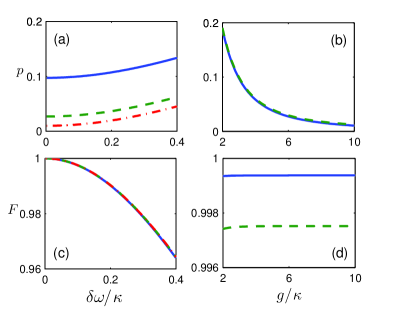
Figure 3: Left column: The loss probability $p$ and the fidelity $F$ as a function of the scaled bandwidth $\delta\omega/\kappa$, with $g=3\kappa$ for the solid line, $g=6\kappa$ for the dashed line, and $g=10\kappa$ for the dash-dotted line. Right column: The loss $p$ and the fidelity $F$ as a function of the scaled atom-cavity coupling rate $g/\kappa$, with $\delta\omega=0.05\kappa$ for the solid line and $\delta\omega=0.1\kappa$ for the dashed line. In the whole figure, we take $\kappa_{h}=\kappa_{v}=\kappa$, $\gamma_{h}=\gamma_{v}=\gamma$, and $\gamma=\kappa$ for simplicity.

Several remarks are in order from this calculation. First, the fidelity $F$ is basically independent of the coupling rate $g$. The loss probability $p$ depends on $g$, but $p$ remains small as long as the variation in $g$ does not reduce $g$ close to zero. This shows that the scheme here allows random variation of the coupling rate $g$ in a significant range. That is a valuable feature for the atomic cavity, as the thermal motion of the atom typically brings it outside of the Lamb-Dicke limit which induces significant random variation of the coupling rate $g$ in current experiments 4 . Second, the scheme here does not require the good cavity limit $g>\kappa$. Independent of the ratio $g/\kappa$, the loss remains small as long as we have the strong coupling condition $g^{2}/\kappa\gamma\gg 1$ (or called the Purcell condition). This is a valuable feature for the solid state cavity as it is typically hard to get $g>\kappa$ for this setup although the Purcell condition $g^{2}/\kappa\gamma\gg 1$ can be satisfied 6 ; 7 . Third, we note that in this scheme the gate infidelity is basically set by the finite pulse bandwidth $\delta\omega/\kappa$, which in principle can be arbitrarily reduced. The intrinsic noise, such as the atomic spontaneous emission (or other kinds of photon loss) only leads to the gate inefficiency errors. Finally, as some explicit parameter estimation, we have the fidelity $F=99.75\%$ and the loss $p=1.3\%$ with the parameters $(g,\kappa,\gamma)/2\pi=(32,4.2,2.6)$ MHz and $\delta\omega=0.1\kappa$, as typical for the atomic cavity 4 ; and $F=99.76\%,$ $p=1.59\%$ with $(g,\kappa,\gamma)/2\pi=(0.66,6,0.001)$ THz and $\delta\omega=0.1g^{2}/\kappa$, as typical for a solid state cavity 6 ; 7 .

In summary, we have proposed a scheme to realize multi-qubit controlled SWAP gates, which have critical application for implementation of both quantum cryptographic protocols and photonic quantum computation. The scheme has a number of nice features that make it robust to practical noise and realizable with the current technology.

We thank Jeff Kimble for helpful discussion. This work was supported by the ARDA under ARO contracts, the NSF award (0431476), and the A. P. Sloan Fellowship.

References

- (1) H. Buhrman, R. Cleve, J. Watrous, and R. de Wolf, Phys. Rev. Lett. 87, 167902 (2001).
- (2) D. Gottesman and I. Chuang, quant-ph/0105032.
- (3) L. M. Duan and H. J. Kimble, Phys. Rev. Lett. 92, 127902 (2004).
- (4) J. McKeever, J. R. Buck, A. D. Boozer, and H. J. Kimble, Phys. Rev. Lett. 92, 143601 (2004); A. Boca et al., Phys. Rev. Lett. 93, 233603 (2004); P. Maunz et al., Phys. Rev. Lett. 94, 033002 (2005).
- (5) A. Imamoglu et al., Phys. Rev. Lett. 83, 4204 (1999).
- (6) E. Waks and J. Vuckovic, Phys. Rev. Lett. 96, 153601 (2006).
- (7) A. Badolato et al., Science 308, 1158 (2005); J. P. Reithmaier et al., Nature 432, 197 (2004); T. Yoshie et al., Nature 432, 200 (2004); J. Vuckovic et al., Appl. Phys. Lett. 82, 3596 (2003).
- (8) There is actually a sign flip of the atomic state with reflection of each pulse, but this sign flip can be easily compensated afterwards by a operation on the atom.
- (9) D. F. Walls, and G. J. Milburn, Quantum Optics (Springer-Verlag, Berlin, 1994).
- (10) L. M. Duan, A. Kuzmich, and H. J. Kimble, Phys. Rev. A 67, 032305 (2003).
- (11) L-M. Duan, J.I. Cirac, P. Zoller, E. S. Polzik, Phys. Rev. Lett. 85, 5643 (2000).
- (12) The fidelity in general depends on the input state, but for different inputs it is of the same order of magnitude.
- (13) E. Knill, R. Laflamme, and G. J. Milburn, quant-ph/0006120; L.-M. Duan and R. Raussendorf, Phys. Rev. Lett. 95, 080503 (2005).