Influence of a tight isotropic harmonic trap on photoassociation in ultracold homonuclear alkali gases

Abstract

The influence of a tight isotropic harmonic trap on photoassociation of two ultracold alkali atoms forming a homonuclear diatomic is investigated using realistic atomic interaction potentials. Confinement of the initial atom pair due to the trap leads to a uniform strong enhancement of the photoassociation rate to most, but also to a strongly suppressed rate for some final states. Thus tighter traps do not necessarily enhance the photoassociation rate. A further massive enhancement of the rate is found for strong interatomic interaction potentials. The details of this interaction play a minor role, except for large repulsive interactions for which a sharp window occurs in the photoassociation spectrum as is known from the trap-free case. A comparison with simplified models describing the atomic interaction like the pseudopotential approximation shows that they often provide reasonable estimates for the trap-induced enhancement of the photoassociation rate even if the predicted rates can be completely erroneous.

I Introduction

Over the past ten years there has been an increasing interest in ultracold atomic and molecular physics. This interest was stimulated by the successful experimental observation of Bose-Einstein condensation (BEC) in dilute atomic gases Anderson et al. (1995). These atomic condensates exhibit many qualitatively new features. Besides their relevance to fundamental quantum statistical and possibly even solid-state questions a further interesting aspect is that the atoms can bind together to form ultracold and even Bose-Einstein condensed molecules Jochim et al. (2003); Regal et al. (2003); Zwierlein et al. (2003).

Although so far the only successful way for achieving a molecular BEC is based on magnetic Feshbach resonances, alternative schemes are still highly desirable, since magnetic Feshbach resonances do not appear to be a universal tool. One of the alternative schemes is photoassociation where two ultracold or Bose-condensed atoms absorb a photon and form a bound excited molecule Lett et al. (1993); Fioretti et al. (1998). Although it was demonstrated that this process generates cold molecules, the yield is small compared to the one obtained by means of magnetic Feshbach resonances. The advantage of photoassociation (and related coherent-control schemes) compared to Feshbach resonances is, however, their assumed wider range of applicability, since there is no need for the occurrence of suitable resonances and thus no requirement for specific magnetic properties of the atoms involved.

Besides simple one-step photoassociation that yields electronically excited molecules there are also resonant or non-resonant multi-step schemes leading to the electronic and possibly even rovibrational ground state. One of the schemes to produce molecules from atoms with help of lasers is, e. g., two-color stimulated Raman adiabatic passage Drummond et al. (2002). The present work discusses only one-photon association explicitly, but it is important to note that the discussed transition matrix elements are direct ingredients for the modeling of more sophisticated schemes like the mentioned two-photon processes.

Photoassociation is also a powerful tool for the investigation of the properties of cold atoms and diatomic molecules. The absorption of the photon typically occurs at large internuclear distances, and thus the photoassociation spectrum provides important information about the long-range part of the molecular potential curves as well as the collisional properties of atoms Abraham et al. (1995); Tiemann et al. (1996); Fioretti et al. (2001); Gutterres et al. (2002).

The cooling of atomic samples is usually achieved in a trap and thus photoassociation experiments in ultra-cold atomic gases are performed in the presence of a trap potential. In most cases these traps are rather shallow so that the corresponding trap frequency $\displaystyle\omega$ is of the order of 100 Hz Schloeder et al. (2003). (Here and in the following the frequency of the trap corresponds to the one in the harmonic approximation). For such a frequency the influence of the trap is expected to be negligible. This may, however, change for very tight traps. In fact, it was pointed out that the atom-molecule conversion process is more efficient, if photoassociation is performed under tight trapping conditions as they are, e. g., accessible in optical lattices Jaksch et al. (2002). The advantage of using tight confinement has stimulated further theoretical investigations and very recently some proposals were made that discuss the possibility of using the trapping potential itself for the formation of molecules Bolda et al. (2005); Koch et al. (2005).

The study of photoassociation in tight optical lattices is of interest by itself, since it is possible to achieve tailored Mott-Insulator states containing a large number of almost identical lattice sites, each filled with exactly two atoms Greiner et al. (2002). The trap frequency of a lattice site in which molecules are produced via photoassociation can be of the order of 100 kHz Rom et al. (2004). The systematic investigation of the influence of a tight isotropic harmonic trap on the photoassociation process of two alkali atoms forming a homonuclear molecule is the topic of this work. Realistic atom-atom interaction potentials are adopted. This allows to check also the range of applicability of the $\delta$-function (pseudopotential) approximation for the description of the photoassociation process.

In the pseudopotential approximations the true atom-atom interaction is replaced by one that reproduces asymptotically the two-body zero-energy s-wave scattering. For this choice of the potential ($\delta$-function) and if the two atoms are placed in a harmonic trap the Schrödinger equation possesses an analytical solution Busch et al. (1998); Idziaszek and Calarco (2005). The validity regime of the pseudopotential approximation has been discussed with respect to the energy levels for trapped atoms in Blume and Greene (2002). It was shown that the use of an energy-dependent pseudopotential (instead of the mostly adopted energy-independent one) gives almost correct energy levels for two harmonically trapped atoms. Whether this simplified model for the atomic interaction is appropriate for the description of photoassociation in a harmonic trap is, however, not immediately evident. Therefore, the present work compares the results obtained using realistic atomic interaction potentials with the ones obtained with either the energy-dependent or -independent pseudopotential.

Photoassociation in tight traps has been studied theoretically before Deb and You (2003). The energy-independent pseudopotential approximation was adopted and only photoassociation into long-range states discussed. Since the present work uses realistic atomic interaction potentials, transitions to all final vibrational states can be considered. This allows to identify two different regimes with respect to the influence of a tight trap on the photoassociation rate as well as (approximate) rules where a transition from one regime to the other is to be expected.

The outline of this work is the following. First, a brief description of the model systems is given in Sec. II. In Sec. III the influence of a tight trap on photoassociation is discussed. This includes after a brief general discussion of the trap influence in Sec. III.1 the derivation of a sum rule in Sec. III.2, the introduction of an enhancement or suppression factor in Sec. III.3, and the discussion of two regimes in Sec. III.4 and III.5. Then the case of repulsive atom-atom interactions is considered in Sec. III.6. The combined influence of trap frequency and atom-atom interaction on photoassociation is investigated in Sec. III.7, the validity of the pseudopotential approximation in Sec. IV. Finally, a discussion and outlook is given in Sec. V. All equations and quantities in this paper are given in atomic units unless otherwise specified.

II The system

Photoassociation of two identical atoms confined in an isotropic harmonic trap and interacting through a two-body Born-Oppenheimer potential $\displaystyle V_{\rm int}(R)$ is considered. The spherical symmetry and harmonicity of the trap allows to separate the center-of-mass and the radial internal motion Busch et al. (1998). The eigenfunctions of the center-of-mass motion are the harmonic-oscillator states. Thus the problem reduces to solving the Schrödinger equation for the radial internal motion

$$\displaystyle\left[\frac{1}{2\mu}\frac{d^{2}}{dR^{2}}\,-\,\frac{J(J+1)}{2\mu R^{2}}\,\right. - V_{\rm int}(R)\,-\,\frac{1}{2}\mu\omega^{2}R^{2}$$ (1)

$$+ \left.E\,\right]\,\Psi(R)\,=\,0\;.$$

In Eq. (1) $J$ denotes the rotational quantum number, $\displaystyle\omega$ is the harmonic trap frequency, and $\displaystyle\mu$ is the reduced mass that is equal to $m/2$ in the present case of particles with identical mass $m$.

In order to compute the photoassociation spectrum the vibrational wave functions $\Psi(R)/R$ are determined for the initial and final molecular states from Eq. (1) with the corresponding Born-Oppenheimer interaction potentials $V_{\rm int}(R)$. The equation is solved numerically using an expansion in $B$ splines. For the investigation of the influence of the trap on the photoassociation rate Eq. (1) is solved for $\omega\neq 0$.

The photoassociation processes most relevant to experiments on ultracold alkali atoms correspond to transitions from two free ground-state atoms (interacting via the ground triplet or singlet potential) to the different vibrational levels of the first excited triplet or singlet state Almazor et al. (1999, 2001); Kemmann et al. (2004). Due to hyperfine interaction, two alkali atoms can also interact via a coherent admixture of singlet and triplet states. This work starts by considering the photoassociative transition between the two triplet states $a^{3}\Sigma^{+}_{u}$ and $1^{3}\Sigma^{+}_{g}$ for ${}^{6}\mbox{Li}$. A corresponding experiment is, e. g., reported in Schloeder et al. (2003). The generality of the conclusions drawn from this specific example are then tested by considering also other atoms (⁷Li and ³⁹K) or modifying artificially the interaction strength, as is discussed below.

For the short-range part of the $a^{3}\Sigma^{+}_{u}$ molecular potential of Li₂ the data in Colavecchia et al. (2003) are used, including the van der Waals coefficients cited therein. In the case of the $1^{3}\Sigma^{+}_{g}$ state data for interatomic distances between $\displaystyle R=4.66\,a_{0}$ and $\displaystyle R=7.84\,a_{0}$ are taken from Linton et al. (1989) and are extended with ab initio values from Schmidt-Mink et al. (1985) for distances between $\displaystyle R=3.25\,a_{0}$ and $\displaystyle R=4.50\,a_{0}$ and between $\displaystyle R=8.0\,a_{0}$ and $\displaystyle R=30.0\,a_{0}$. The van der Waals coefficients from Marinescu and Dalgarno (1995) are used. For a $\Sigma$ to $\Sigma$ molecular dipole transition the selection rule is $J=J^{\prime}\pm 1$. Assuming ultracold atomic gases the atoms interact initially in the $\displaystyle J^{\prime}=0$ state of the $a^{3}\Sigma^{+}_{u}$ potential. The dipole selection rule leads then to transitions to the $\displaystyle J=1$ states of $1^{3}\Sigma^{+}_{g}$. With the given potential-curve parameters a solution of Eq. (1) in the absence of a trap ($\omega=0$) yields for the fermionic ⁶Li atoms 10 and 100 vibrational bound states for the $a^{3}\Sigma^{+}_{u}$ ($J^{\prime}=0$) and the $1^{3}\Sigma^{+}_{g}$ ($J=1$) states, respectively. In the case of the bosonic ⁷Li atoms there are 11 and 108 vibrational bound states for the $a^{3}\Sigma^{+}_{u}$ ($J^{\prime}=0$) and the $1^{3}\Sigma^{+}_{g}$ ($J=1$) states, respectively.

The electronic dipole moment $D(R)$ for the transition $a\,^{3}\Sigma^{+}_{u}\rightarrow 1\,^{3}\Sigma^{+}_{g}$ of Li was calculated Vanne with a configuration interaction (CI) method for the two valence electrons using the code described in Vanne and Saenz (2004). The core electrons were described with the aid of the Klapish model potential with the parameters given in Magnier et al. (1999) and polarization was considered as discussed in Dumitriu et al. (2006). The resulting $D(R)$ (and its value in the separated atom limit) is in good agreement with literature data Schmidt-Mink et al. (1985); Ratcliff et al. (1987); Pipin and Bishop (1991); Marinescu and Dalgarno (1995).

In the limit of zero collision energy the interaction between two atoms can be characterised by their s-wave scattering length $\displaystyle a_{\rm sc}$. Its sign determines the type of interaction (repulsive or attractive) and its absolute value the interaction strength. For a given potential curve the s-wave ($J^{\prime}=0$) scattering length can be determined using the fact that at large distances the scattering wave function describing the relative motion (for $\omega=0$ and very small collision energies) reaches an asymptotic behavior of the form

$$\Psi_{E}(R)=\sqrt{\frac{k}{\pi E}}~{}\sin\left[k(R-a_{\rm sc})\right]\;.$$ (2)

In the present numerical approach discretised continuum states are obtained, since the wave-function calculation is performed within a finite $\displaystyle R$ range, i. e. in the interval $[0,R_{\rm max}]$. Only wave functions that decay before or have a node at $R_{\rm max}$ are obtained. From the analysis of the lowest lying discretised continuum state the scattering length $a_{\rm sc}$ is obtained by the use of the relation $\displaystyle a_{\rm sc}=R_{\rm max}-\frac{\pi}{k}$ with $\displaystyle k=\sqrt{2\mu E}$ Julienne (1996). A variation of $R_{\rm max}$ changes the continuum discretization and therefore results in $R_{\rm max}$-dependent lowest lying continuum solutions $\Psi_{E_{0}}$. The scattering length extracted from $\Psi_{E_{0}}$ converges, however, to a constant value as $R_{\rm max}$ increases and $E_{0}$ approaches zero. Using this method and the adopted potential curves the scattering length values $\displaystyle a_{\rm sc}=-2030\,a_{0}$ and $\displaystyle a_{\rm sc}=-30\,a_{0}$ are obtained for ⁶Li and ⁷Li, respectively. These values agree well with the experimental ones: $a_{\rm sc}=(-2160\pm 250)\,a_{0}$ (⁶Li) and $a_{\rm sc}=(-27.6\pm 0.5)\,a_{0}$ (⁷Li) Abraham et al. (1996a).

The interaction of two ultracold ⁶Li atoms is strongly, the one of ⁷Li weakly attractive, as is reflected by the large and small but negative scattering lengths. In the case of two identical fermionic ⁶Li atoms the asymmetry requirement of the total wave function excludes s-wave scattering. Thus the present results are more applicable for two ⁶Li atoms in different hyperfine states (where the admixture of a singlet potential would, however, usually modify the scattering length), but are actually meant as a realistic example for a very large negative scattering length, i. e. strong attraction. In order to further check the generality of the results also the formation of ³⁹K₂ is investigated as an example for a small repulsive interaction. In this case photoassociation starting from two potassium atoms interacting via the singlet $X^{1}\Sigma^{+}_{g}$ ground state and transitions into the $A^{1}\Sigma_{u}^{+}$ state are considered. This process is not only experimentally relevant Nikolov et al. (1999), but is at the same time an even further check of the generality of the conclusions obtained from the investigation of the transitions between triplet states in $\mbox{Li}_{2}$.

The data for constructing the relevant potential curves for ³⁹K₂ are taken from col ; Amiot et al. (1995); Wang et al. (1997). The resulting potential curve for the $X^{1}\Sigma^{+}_{g}$ state yields a scattering length $a_{\rm sc}\approx+90\,a_{0}$. This is in reasonable agreement with the experimental value given in Williams et al. (2000) where $a_{\rm sc}$ is found to be lying between $+90\,a_{0}$ and $+230\,a_{0}$.

Instead of selecting additional atomic pairs that could represent examples for other values of the scattering length, the sensitivity of the s-wave interaction on the position of the least bound state is used to generate artificially a variable interaction strength. The scattering length is thus modified by a variation of the particle mass. The strong mass dependence of the scattering length is already evident from its change from $-2030\,a_{0}$ to $-30\,a_{0}$ for the isotopes ⁶Li and ⁷Li, respectively. Experimentally, a strong variation of the interaction strength can be realized by the aid of magnetic Feshbach resonances Loftus et al. (2002); Regal and Jin (2003).

III Photoassociation in an isotropic harmonic trap

III.1 Photoassociation in a trap

While Eq. (1) yields in the trap-free case ($\omega=0$) both bound (vibrational) and continuum (dissociative) states, the harmonic trap potential changes the energy spectrum to a purely discrete one, as is sketched in Fig. 1.

Figure 1: Sketch of the photoassociation process for ${}^{6}\mbox{Li}_{2}$ in the presence of a trap (not to scale). With the aid of a laser photoassociation is induced from the first trap-induced bound state ($\displaystyle v^{\prime}=10$) of the $a^{3}\Sigma^{+}_{u}$ state into some vibrational level $\displaystyle v$ of the $1^{3}\Sigma^{+}_{g}$ state. Different laser frequencies $\nu_{i}$ couple the same initial state to different final states.

Considering the concrete example of two ⁶Li atoms where the $a^{3}\Sigma^{+}_{u}$ state supports the 10 vibrational bound states $v^{\prime}=0$ to 9, $v^{\prime}=10$ ($J^{\prime}=0$) denotes the first state that results from the trap-induced continuum discretization. This (first trap-induced) state describes the initial state of two spin-polarized ⁶Li atoms interacting via the $a^{3}\Sigma^{+}_{u}$ potential curve, if a sufficiently cold atomic gas in an (adiabatically turned-on) harmonic trap is considered. In the present work photoassociation (by means of a suitably tuned laser) from this initial state to one of the vibrational states $v$ of the $1^{3}\Sigma^{+}_{g}$ potential is investigated as a function of the trap frequency $\omega$. In view of the already discussed relevant dipole-selection rule the final state possesses $J=1$ and in the following $J^{\prime}=0$ and $J=1$ is tacitly assumed. The strength of the photoassociation transition to final state $v$ is given by the rate Côté and Dalgarno (1998)

$$\Gamma_{v}(\omega)=4\pi^{2}\mathcal{I}\,I^{v}(\omega)$$ (3)

where $\mathcal{I}$ is the laser intensity and

$$I^{v}(\omega)=\left|\int\limits_{0}^{\infty}\>\Psi^{v}(R;\omega)\>D(R)\>\Psi^{\rm 10^{\prime}}(R;\omega)\>{\rm d}R\right|^{2}\;.$$ (4)

In Eq. (4) $\Psi^{v}(R)/R$ and $\Psi^{\rm 10^{\prime}}(R)/R$ are the vibrational wave functions of the final and initial state, respectively. Since the radial density is proportional to $|\Psi|^{2}$, it is convenient to discuss $\Psi$ instead of the true vibrational wave function $\Psi(R)/R$. This will be done in the following where $\Psi$ is for simplicity called vibrational wave function. Finally, $D(R)$ is the ($R$-dependent) electronic transition dipole matrix element between the $a^{3}\Sigma^{+}_{u}$ and the $1^{3}\Sigma^{+}_{g}$ state of $\mbox{Li}_{2}$ introduced in Sec. II. $D(R)$ is practically constant for $R>25\,a_{0}$. Eq. (4) is only valid within the dipole approximation. The latter is supposed to be applicable, if the photon wavelength is much larger than the extension of the atomic or molecular system. The shortest photoassociation laser wavelength corresponds to the transition to the highest-lying vibrational state and is thus approximately the one of the atomic (2 ²S $\rightarrow$ 2 ²P transition), $\lambda=12680\,a_{0}$. Although the spatial extent of some of the final vibrational states (and of course the initial state in the case of shallow traps) has a similar or even larger extent, beyond dipole approximation effects are neglected in this work.

The key quantity describing the photoassociation rate to different vibrational states $v$ or for variable trap frequency $\omega$ is $I^{v}(\omega)$ on whose calculation and discussion this work concentrates. It is important to note that also in the case of more elaborate laser-assisted association schemes like stimulated Raman processes that involve (virtual) transitions to the $v$ states the transition rate is proportional to $I^{v}(\omega)$.

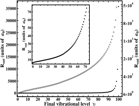
Figure 2: The classical outer turning points of the vibrational levels of the $1\,^{3}\Sigma_{g}^{+}$ state of ⁶Li₂ are shown on a linear (solid circles, left scale and insert) and on a logarithmic scale (empty circles, right scale).

According to Eq. (4) the photoassociation rate depends for transitions between long-range states on the Franck-Condon factors between the initial and final nuclear wave functions, if $D(R)$ is practically constant for large $R$. In the case of alkali atoms the interaction potentials of the electronic states can be very long ranged and can contain numerous rovibrational bound states. Fig. 2 shows, e. g., the classical outer turning points $R_{\rm out}$ of the 100 ($J=0$) vibrational bound states of ⁶Li₂ supported by the final-state electronic potential curve $1^{3}\Sigma^{+}_{g}$. The orthogonality of the states is achieved by the occurrence of $v^{\prime}$ nodes. As $v^{\prime}$ increases the wavefunctions consist of a highly oscillatory short range part with small overall amplitude that covers the range of the $v^{\prime}-1$ wavefunction and a large outermost lobe. The $1^{3}\Sigma^{+}_{g}$ state is very long ranged, since its leading van der Waals term is $\displaystyle-C_{3}/R^{3}$. The initial electronic state $a^{3}\Sigma^{+}_{u}$ with leading $\displaystyle-C_{6}/R^{6}$ van der Waals term is shorter ranged. Fig. 3 shows the initial vibrational state for ⁶Li as a function of the trap frequency. This first trap-induced bound state possesses $v$ nodes (here $v=10$) that are located in the $R$ range of the last trap-free bound state ($v=9$). The overall amplitude in this about $25\,a_{0}$ long interval is very small and most of the wavefunction is distributed over the harmonic trap.

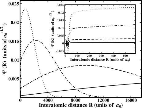
Figure 3: Wave functions of the initial $a\,^{3}\Sigma_{u}^{+}$ state of ${}^{6}\mbox{Li}_{2}$ for trap frequencies $\omega=2\pi\times\mbox{1kHz}$ (solid), $\omega=2\pi\times\mbox{10kHz}$ (dashes), $\omega=2\pi\times\mbox{100kHz}$ (chain), and $\omega=2\pi\times\mbox{500kHz}$ (dots). (The insert shows the small $\displaystyle R$ range on an enlarged scale.)

The squared transition dipole moments $\displaystyle I^{v}(\omega)$ are shown for ${}^{6}\mbox{Li}$ in Fig. 4(a) for three different trap frequencies $\displaystyle\omega$.

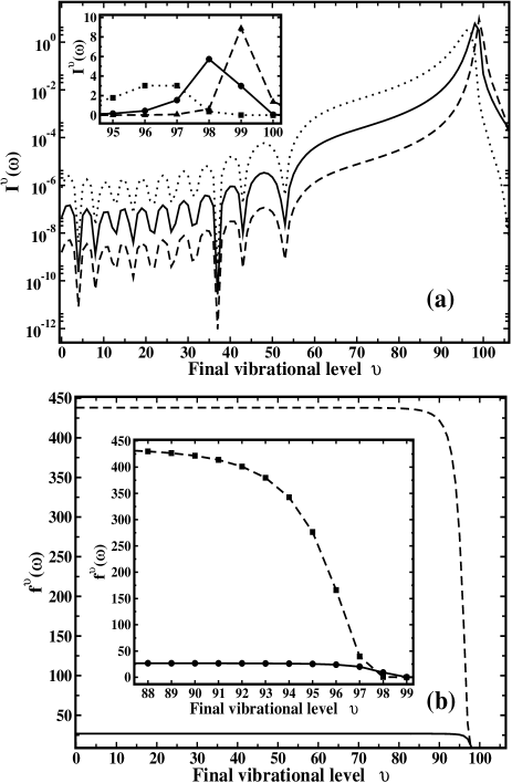
Figure 4: (a) The squared dipole transition moments $\displaystyle I^{v}(\omega)$ describing transitions from the trap-induced ($v^{\prime}=10$) initial $a^{3}\Sigma^{+}_{u}$ state to the vibrational manifold ($v$) of the $1^{3}\Sigma^{+}_{g}$ state of ${}^{6}\mbox{Li}_{2}$ are shown for the trap frequencies $\omega=2\pi\times 1\mbox{kHz}$ (dashes), $\omega=2\pi\times 10\mbox{kHz}$ (solid), and $\omega=2\pi\times 100\mbox{kHz}$ (dots). The insert shows the transitions to $v=95$ to 100 on an enlarged scale. For a better visibility the discrete transitions (marked explicitly with different symbols in the insert) are plotted as continuous lines. (b) The ratio $\displaystyle f^{v}(\omega)$ [defined in Eq. (6)] is shown for $\displaystyle\omega=2\pi\times 10\,\mbox{kHz}$ (solid) and $\omega=2\pi\times 100\,\mbox{kHz}$ (dashes) as a function of the final vibrational level $v$. (As in (a) the discrete points are connected by lines to guide the eye.) The insert shows the transitions to $v=88$ to 99 on a magnified scale.

As mentioned before, the final vibrational levels with $v>99$ are trap-induced bound states and exist only due to the continuum discretization in the presence of a trap. If the trap would be turned-off (adiabatically) after photoassociation to such a level, the trap induced dimer would immediately dissociate (without the need for any (radiative or non-radiative) coupling to some dissociative state).

For a fixed trap frequency the photoassociation rate generally increases as a function of the final vibrational level $v$, but for small $v$ an oscillatory behavior is visible. These oscillations are a consequence of the nodal structure of the initial-state wave functions describing the atom pair. The 10 nodes (for the shown example of ⁶Li) of the initial-state wave function lead to exactly 10 dips in photoassociation spectrum. Their exact position depends on the interference with the nodal structure of the final-state wave functions. The oscillatory structure of $I^{v}(\omega)$ ends at about $v=55$ and beyond that point the rate increases by orders of magnitude, before a sharp decrease is observed close to the highest lying vibrational bound state ($v=99$). The absence of oscillatory behavior is a clear signature that for those transitions (in the present example for transitions into states with $v>55$) the Franck-Condon factors are determined by the overlap of the outermost lobe of the initial state with the one of the final state.

The comparison of $I^{v}(\omega)$ for the different trap frequencies shown in Fig. 4(a) indicates a very systematic trend. The transition probabilities to most of the vibrational bound states increases with increasing trap frequency. This is in accordance with simple confinement arguments, since a tighter trap confines the atoms in the initial state to a smaller spatial region. Due to the special properties of harmonic traps, this confinement translates directly into a corresponding confinement of the pair density (see Eq.(1)). The probability for atom pairs to have the correct separation for the photoassociative transition is thus expected to increase for tighter confinements, since a larger Franck-Condon overlap of the now more compact initial state with the bound molecular final state is expected. However, for the vibrational final states close to and above the (trap-free) dissociation threshold a completely different behavior is found. In this case the photoassociation rate decreases with increasing trap frequency, as can be seen especially from the insert of Fig. 4(a). In fact, a sharp cut-off of the transition rate is observed. The transitions to the states that possessed the largest photoassociation rate for small trap frequencies are almost completely suppressed for large trap frequencies. Clearly, the simple assumption “a tighter trap leads to a higher photoassociation rate due to an increased spatial confinement” is only partly true. The fact that this assumption cannot be valid for all final states can be substantiated by means of a general sum-rule that is derived and discussed in the following subsection.

III.2 Sum rule

Performing a summation (including for $\omega=0$ an integration over the dissociative continuum) over all final vibrational states (using closure) yields

$$\widetilde{I}(\omega)\;=\;\sum\limits_{v=0}^{\infty}\>I^{v}(\omega)\;=\;\int\limits_{0}^{\infty}\>\Psi^{\rm 10^{\prime}}(R;\omega)\,D^{2}(R)\,\Psi^{\rm 10^{\prime}}(R;\omega)\>{\rm d}R\;.$$ (5)

While the electronic transition dipole moment $D(R)$ depends clearly on $R$ for small internuclear separations, it reaches its asymptotic value (the sum of the electronic dipole transition moments of two separated atoms, $D_{\rm at}$) at some $R$ value that is much smaller than the typical spatial extend of the final vibrational states with the largest transition amplitudes. (In the example of Li₂ this asymptotic limit is reached at about $25\,a_{0}$.) If the largest photoassociation amplitudes result from transitions to final states whose wave functions are mostly located outside this $R$ range, the integral in Eq. (5) is dominated by the $R$ regime in which $D(R)$ is constant. In this case $D^{2}$ can be taken out of the integral and normalization of the initial wave function assures $\widetilde{I}(\omega)\approx\widetilde{I}=D_{\rm at}^{2}$.

Consequently, for all trap frequencies that are too small to confine the atoms into a spatial volume that is comparable to the atomic volumes (leading to $D(R)\neq\,D_{\rm at}$) and thus for all traps relevant to this work (and presently experimentally achievable) the total dipole transition moment $\widetilde{I}$ is to a good approximation independent of the trap frequency $\omega$. Therefore, changing the trap frequency can only redistribute transition probabilities between different final vibrational states. Increasing the transition rate to one final state must be compensated by a decrease of the transition probability to one or more other vibrational states.

A conservative estimate of the minimum and maximum influence of a harmonic trap on the photoassociation rate is obtained from $\widetilde{I}_{\rm min}=D_{\rm min}^{2}$ and $\widetilde{I}_{\rm max}=D_{\rm max}^{2}$, respectively, where $D_{\rm min}$ ($D_{\rm max}$) is the minimum (maximum) value of the molecular electronic transition dipole moment.

The sum-rule values obtained numerically for the trap frequencies shown in Fig. 4(a) are $\widetilde{I}(\omega=2\pi\times 1\,$kHz$)=11.127222$, $\widetilde{I}(\omega=2\pi\times 10\,$kHz$)=11.12723$, and $\widetilde{I}(\omega=2\pi\times 100$ kHz$)=11.1273$. This may be compared to the value $\lim_{R\rightarrow\infty}\,|D(R)|^{2}=D_{\rm at}^{2}\ =|D_{\rm 2s-2s}+D_{\rm 2s-2p}|^{2}=|D_{\rm 2s-2p}|^{2}=11.1272213$ obtained from the calculation described in Sec.  II. Clearly, the sum-rule (5) can also be used as a test for the correctness of numerical calculations. The very small deviations from the predicted sum-rule value may, however, not only be a result of an inaccuracy of the present numerical approach, but also reflect the (small) $R$ dependence of $D(R)$ that allows some $\omega$ dependence of the total photoassociation rate. This interpretation is supported by the fact that the numerically found deviations monotonously increase with increasing frequency $\omega$. Larger values of $\omega$ lead to a spatially more confined $\Psi^{\rm 10^{\prime}}(R;\omega)$ which in turn probes more of the $R$-dependent part of $D(R)$. Since $D(R)$ approaches $D(R=\infty)=D_{\rm at}$ from above, a small increase of $\widetilde{I}$ is expected for increasing trap frequencies. As is evident from Fig. 4 (a) (especially the insert), the sum-rule fulfillment is achieved by a drastic decrease of the photoassociation rate to the highest lying final states. This compensates the trap-induced increased rate to the lower lying states. Since the rate to the highest lying states is orders of magnitude larger than the one to the low-lying states, the reduced transition probability of a small number of states can easily compensate the substantial increase by orders of magnitude observed for the large number of low-lying states.

From Eq. (5) it is clear that in those cases where most of the contribution to the sum rule stems from the $R$ range where $D(R)$ is practically constant, there is also no influence of the initial-state wave function. Taking $D$ out of the integral yields always the self-overlap of the initial-state wave function and thus unity. This is important, since it indicates that the sum-rule value is also (approximately) independent of the atom-atom interaction potential.

III.3 Enhancement and suppression factor $f^{v}$

In order to quantify the effect of a tight harmonic trap on the photoassociation rate and to get rid of its variation as a function of the final-state vibrational level $v$ (that is due to the nodal structure and clearly visible in Fig. 4(a) especially for smaller $v$) the ratio

$$f^{v}(\omega)=\frac{I^{v}(\omega)}{I^{v}(\omega_{\rm ref})}\;.$$ (6)

may be introduced. It describes the relative enhancement ($f^{v}(\omega)>1$) or suppression ($f^{v}(\omega)<1$) of the photoassociation rate to a specific final state $v$ at a given trap frequency $\omega$ with respect to the reference frequency $\omega_{\rm ref}$. Although it may appear to be most natural to choose the trap-free case as reference ($\omega_{\rm ref}=0$), a finite value offers some advantages. First, a different normalization applies to $\omega=0$ and $\omega\neq 0$, since in one case it is free-to-bound transitions, while it is bound-to-bound transitions otherwise. Second, from a numerical point of view it is more convenient to treat both cases the same way and to avoid the variation of the box boundary $\displaystyle R_{\rm max}$ that would otherwise be necessary for the trap-free case. Finally, it may be argued that a non-zero trap reference state is in fact more relevant to typical photoassociation experiments with ultracold alkali atoms, since most of them are anyhow performed in traps. In the present work $\omega_{\rm ref}=2\pi\times 1\,\mbox{kHz}$ was chosen. This value is sufficiently small to represent typical shallow traps in which the influence of the trap on photoassociation is supposedly (at least to a good approximation) negligible. On the other hand, it allows to calculate the transition dipole moments with reasonable numerical efforts and thus sufficient accuracy.

The ratio $f^{v}(\omega)$ is shown for two different trap frequencies $\omega$ in Fig. 4(b). For most of the vibrational final states a simple constant regime is observed, i. e. the ratio $f^{v}(\omega)$ is independent of $v$ for all except the highest lying states. This constant regime is followed by a relatively sharp cut-off beyond which the ratio $f^{v}(\omega)$ is very small. In the constant regime a 100 kHz trap leads to an enhancement by almost 3 orders of magnitude.

Comparing the results for different $\omega$ one notices that in the range of final states where a constant behavior (with respect to $v$) is observed, a tighter trap leads to an increased photoassociation rate, trap-induced enhanced photoassociation (EPA). Due to the cut-off this is, however, not true, if the last vibrational states are considered. Since the range of constant behavior shrinks with increasing trap frequency, there is an increasing range of vibrational states for which a tighter trap leads to a smaller photoassociation rate compared to a shallower trap. In this case trap-induced suppressed photoassociation (SPA) occurs. This effect is especially visible from the insert of Fig. 4(a). The physical origin of the two different regimes (constant vs. cut-off) and their $\omega$ dependence is discussed separately in the following two subsections.

III.4 Constant regime

Since in the constant regime the ratio $f^{v}(\omega)$ is completely independent of the final state level $v$, its value (for a given $\omega$) and constancy (as a function of $v$) must be a consequence of the influence of the trap on the initial state. The initial-state wave function for a ⁶Li atom pair was shown for three different trap frequencies in Fig. 3. A view on the complete wave function reveals directly the confinement of the wave function to a smaller spatial volume, if the trap frequency is increased. However, on this scale the variation of the wave function at a specific value of $R$ appears to be quite complicated. Thus it is not at all clear why the enhancement factor $f^{v}$ has for so many states a constant value. A closer look at smaller internuclear separations (insert of Fig. 3) reveals that besides the initial oscillatory part confined to the effective range of the atom-atom interaction potential there is a relatively large $R$ interval in which the wave functions for the different trap frequencies vary linearly with $R$. In this case the slope is very small and the wave function is thus almost constant. If the Franck-Condon integral is determined only by the value of the initial-state wave function in this $R$ window, it produces an almost undistorted image of the final-state wave function.

However, for the ratio $f^{v}(\omega)$ this final-state dependence disappears. The reason is that in the $R$ range where the initial-state wave function is almost constant, its variation with the trap frequency is also $R$ independent, as can be seen from the insert of Fig. 3. In other words, one finds $\displaystyle\Psi^{\rm 10^{\prime}}(R;\omega)=C(\omega)\cdot\Psi^{\rm 10^{\prime}}(R;\omega_{\rm ref})$. If no final-state dependence occurs, the constant $C(\omega)$ is related to the ratio $f$ via $f_{c}(\omega)=C^{2}(\omega)$. The validity of this argument for the occurrence of a constant ratio $f$ can thus be checked (and visualized) in the following way. Together with the correct wave function $\displaystyle\Psi^{\rm 10^{\prime}}(R;\omega)$ the approximate one, $~{}\sqrt{f_{c}(\omega)}~{}\cdot~{}\Psi^{\rm 10^{\prime}}(R;\omega_{\rm ref})$, is plotted where $f_{c}(\omega)$ is the value of the factor $f$ in the constant regime. A convenient way to determine $f_{c}(\omega)$ follows from the observation that the constant regime always starts at $v=0$. Thus $f_{c}(\omega)=f^{v=0}(\omega)$ is the most straightforward way of $f_{c}(\omega)$ determination. In Fig. 5 the correct wave function $\displaystyle\Psi^{\rm 10^{\prime}}(R;\omega)$ is plotted together with the approximate wave function $~{}\sqrt{f_{c}(\omega)}~{}\cdot~{}\Psi^{\rm 10^{\prime}}(R;\omega_{\rm ref})$ for the trap frequency $\displaystyle\omega=2\pi\times\mbox{100kHz}$.

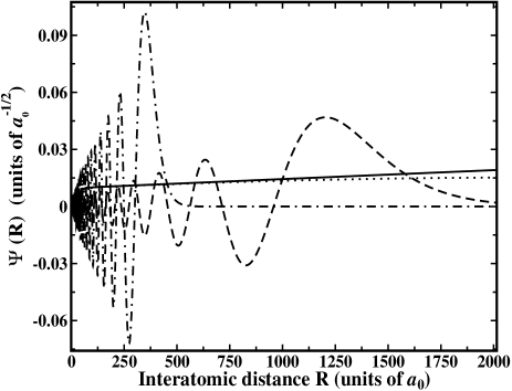
Figure 5: Illustration of the constant photoassociation regime. The initial-state wave function $\Psi^{\rm 10^{\prime}}(R;\omega=100)$ (dots) and an approximation to it, $\sqrt{f_{c}(\omega=100)}\cdot\Psi^{\rm 10^{\prime}}(R;\omega=1)$ (solid), are shown together with the final-state vibrational wave functions for $\displaystyle v=88$ (chain) and $\displaystyle v=94$ (dashes).

The agreement between the two wave functions is clearly good in the shown range of $R$ values, but it is better for small $R$, since at about $R=500\,a_{0}$ the two wave functions start to disagree. Below $R=500\,a_{0}$ the two wave functions agree completely with each other, even in the very short $R$ range where they possess an oscillatory behaviour.

The key for understanding the occurrence of the constant regime is that a variation of the trap frequency modifies the spatial extent of the initial-state wave function, but leaves its norm and nodal structure preserved. As a consequence, the wave function changes qualitatively only in the large $R$ range, while in the short range only the amplitude varies (by factor $C(\omega)$). The reason for this behaviour is that at small $R$ the wave function is practically shielded from the trap potential by the dominant atom-atom interaction.

Fig. 5 shows also two final-state wave functions ($v=88$ and 94). According to Fig. 4 (b) the transition to $v=88$ belongs still to the constant regime ($f^{88}(\omega)\approx f_{c}(\omega)$), though to its very end. The transition to $v=94$ does on the other hand not belong to this regime, since for the considered trap frequency $f^{94}(\omega)<f_{c}(\omega)$. As is evident from Fig. 5, a constant ratio $f^{v}(\omega)$ is observed as long as the final-state wave function $v$ is completely confined within an $R$ range in which the approximation $\displaystyle\Psi^{\rm 10^{\prime}}(R;\omega)\approx C(\omega)\cdot\Psi^{\rm 10^{\prime}}(R;\omega_{\rm ref})$ is well fulfilled. This is (for $\omega=2\pi\times\mbox{100kHz}$) the case for $v=88$ for which the wave function is confined within $R<600\,a_{0}$, but not for $v=94$ whose outermost lobe has its maximum at about $1350\,a_{0}$. Since the $R$ range in which the initial-state wave function can be approximated in the here discussed fashion decreases with increasing trap frequency, the range of $v$ values for which $f^{v}(\omega)\approx f_{c}(\omega)$ is valid diminishes with increasing trap frequency.

The following rule of thumb is found to determine those vibrational levels $v$ for which the relation $f^{v}(\omega)\approx f_{c}(\omega)$ starts to break down. For trap frequencies $\displaystyle\omega_{1}$ and $\displaystyle\omega_{2}$ (with $\displaystyle\omega_{2}>\omega_{1}$) one may define a difference $\Delta$ that quantifies the deviation of $C\cdot\Psi^{\rm 10^{\prime}}(R;\omega_{\rm 1})$ and $\Psi^{\rm 10^{\prime}}~{}(R;\omega_{\rm 2})$ as $\Delta(R)~{}=~{}C\cdot~{}\Psi^{\rm 10^{\prime}}~{}(R;\omega_{\rm 1})~{}-~{}\Psi^{\rm 10^{\prime}}~{}(R;\omega_{\rm 2})$ where $\displaystyle C=\sqrt{f_{c}(\omega_{2})}$. For example, in Fig. 5 the difference $\Delta(R)$ is the distance between the solid curve and the dotted one. The relation $f^{v}(\omega)\approx f_{c}(\omega)$ breaks down for those final states $v$ whose classical turning point lies beyond $R_{0}$. $R_{0}$ itself is determined by $\Delta(R>R_{0})\gtrsim 10^{-3}$. In other words, if the last lobe of the final wave function overlaps substantially with a region where the deviation defined by $\Delta$ is larger than about $10^{-3}$, a clear deviation from the constant regime is to be expected.

III.5 Cut-off regime

Once the constant regime of the ratio $f^{v}$ (for a given trap frequency) is left, $f^{v}$ is steadily decreasing with $v$, as is apparent from Fig. 4 (b). The photoassociation rate displays then a rather sharp cut-off behavior (see insert of Fig. 4 (a)). The most loosely bound vibrational states of the final electronic state have in the trap-free case the largest rate but possess a very small one in very tight traps. For those high-lying states the wave functions have a very highly oscillatory behavior for short $R$ values and a large lobe close to the classical turning point. This outermost lobe determines the Franck-Condon integral, if the initial-state wave function is sufficiently smooth in this $R$ range. In Fig. 6

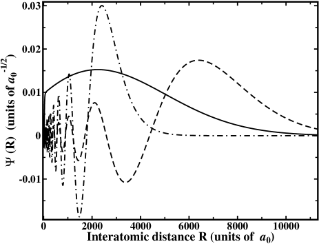
Figure 6: Illustration of the cut-off regime for a 100 kHz trap. The initial-state wave function $\displaystyle\Psi^{\rm 10^{\prime}}(R;100)$ (solid) is shown together with the two final-state wavefunctions for $v=96$ (chain) and $v=98$ (dashes).

the initial-state wave function is shown together with the ones for $v=96$ and 98 (for $\displaystyle\omega=2\pi\times\mbox{100kHz}$).

It is evident from Fig. 6 that for $\displaystyle v=96$ the overlap of the initial wave function with the last lobe of the final state is very large. In fact, for this trap frequency the overlap reaches its maximum for $v=96$ and $97$ (see Fig. 4 (a)), despite the fact that the trap-induced relative enhancement factor $f^{v}(\omega)$ is small (Fig. 4 (b)). In the case of $v=98$ the transition rate is not only clearly smaller than for $v=96$ or $97$, but it is also much smaller than the rate obtained for the same level at much lower trap frequencies (10 or 1 kHz). Clearly, one has $f^{v=98}(\omega)<1$ and thus for $\displaystyle\omega=2\pi\times\mbox{100kHz}$ the level $v=98$ represents an example for a trap-induced suppressed rate (SPA) in contrast to the usually expected enhanced photoassociation in a trap (EPA, $f^{v}(\omega)>1$). From Fig. 6 it is clear that the reason for the small transition rate to $v=98$ is due to the fact that the outermost lobe of the $v=98$ state lies mostly outside the $R$ range in which the initial-state wave function is non-zero. The least bound state (in the trap free case), $v=99$, possesses an even smaller photoassociation rate, since in this case the outermost lobe lies practically completely outside the non-zero $R$ range of the initial-state wave function. Due to the imperfect cancellation of the oscillating contributions from the inner lobes, the photoassociation rate for $v=99$ is very small, but non-zero.

Increasing the trap frequency even more will confine the initial-state wave function to a smaller $R$ range and thus SPA occurs for smaller $v$ values. The origin of the suppression is in fact a quite remarkable feature, since from Fig. 6 it is clear that the trap has practically no influence on the final states, even if one considers the highest-lying ones that have very tiny binding energies. This is still true, if the spatial extent of the final state is much larger than the one of the trap potential. This may be interpreted as a shielding of the trap potential by the molecular (atom-atom interaction) potential. The reason for the different shielding experienced by the initial and the final states is not only due to the fact that the former lies above the dissociation threshold, since then the photoassociation rate should dramatically increase, if transitions into the purely trap-induced bound states of the final electronic state are considered. This is, however, not the case as can be seen for the states $v>99$ in Fig. 4 (a). The different shielding is due to the inherently different long-range behaviors of the two electronic potential curves describing the initial ($a^{3}\Sigma^{+}_{u}$) and the final ($1^{3}\Sigma^{+}_{g}$) state. If one introduces the crossing point $\displaystyle R_{c}$ of the long range part of the van der Waals potential with the one of the inverted harmonic trap, it is defined by equating $\displaystyle C_{n}/R_{c}^{n}$ and $\displaystyle\frac{1}{2}\mu\omega^{2}R_{c}^{2}$ where $C_{n}$ is the corresponding leading van der Waals coefficient. At the point $\displaystyle R_{c}$ the trap potential starts to dominate. For example, in the case of the trap frequency $\omega=2\pi\times\mbox{10kHz}$ one finds $\displaystyle R_{c}\approx+825\,a_{0}$ and $\displaystyle R_{c}\approx+17700\,a_{0}$ for $a^{3}\Sigma^{+}_{u}$ and $1^{3}\Sigma^{+}_{g}$ of Li₂, respectively.

III.6 $\displaystyle I^{v}(\omega)$ for a repulsive interaction

In order to check the main conclusions of the results obtained for ⁶Li₂ also the formation of ³⁹K₂ is investigated. While for ⁶Li a photoassociation process between triplet states was considered, a transition between the $X^{1}\Sigma^{+}_{g}$ and the $A^{1}\Sigma_{u}^{+}$ states is chosen for ³⁹K. In contrast to the large negative scattering length of two ⁶Li atoms interacting via the $a^{3}\Sigma^{+}_{u}$ potential two ³⁹K ground-state atoms interact via a small positive s-wave scattering length. The obtained results for the squared transition dipole moments $I^{v}(\omega)$ are qualitatively very similar to the results obtained for ⁶Li₂. This includes the existence of a constant regime of $f^{v}(\omega)$ followed by a pronounced decrease for the highest-lying vibrational states, the cut-off. The rule of thumb for predicting the range of $v$ values for which a constant ratio $f^{v}$ is observed does also work in this case. ³⁹K₂ shows thus trap-induced suppressed photoassociation for the highest lying states with a sharp cut-off in the $I^{v}(\omega)$ spectrum very much like ⁶Li₂. Therefore, the results are not explicitly shown for space reasons.

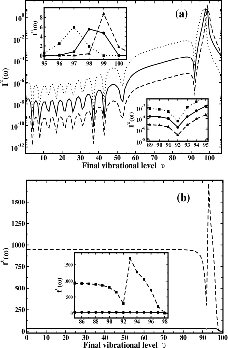
Figure 7: As Fig. 4 but the scattering length is artificially changed to $a_{\rm sc}=+850\,a_{0}$ (see text for details). The additional insert in the right bottom corner of (a) shows the range $v=89$ to $v=95$ on an enlarged scale.

For a more systematic investigation of the influence of the scattering length $a_{\rm sc}$ and thus the type of interaction (sign of $a_{\rm sc}$) and its strength (absolute value of $a_{\rm sc}$) the mass of the Li atoms is varied. The mass variation allows for an in principle continuous (though non-physical) modification of $a_{\rm sc}$ from very large positive to negative values. With increasing mass an increasing number of bound states is supported by the same potential curve. Since $a_{\rm sc}$ is sensitive to the position of the least bound state, even a very small mass variation has a very large effect, if a formerly unbound state becomes bound. For example, an increase of the mass of ⁶Li by 0.3% changes $a_{\rm sc}$ from $-2030\,a_{0}$ to about $+850\,a_{0}$. The (for ⁶Li unbound) 11th vibrational state becomes weakly bound. A further increase of the mass increases its binding energy until it reaches the value for ⁷Li. It is also possible to modify $a_{\rm sc}$ from $-2030\,a_{0}$ to $+850\,a_{0}$ by lowering the mass of ⁶Li. A larger mass variation is required (about 18 %) but the number of bound states remains unchanged. In this case the large positive value of $a_{\rm sc}$ indicates that the 10th bound state is, however, only very weakly bound and a further small decrease of the mass will shift it into the dissociative continuum.

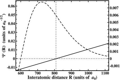
Figure 8: For ⁶Li₂ (the scattering length in the initial channel is modified to $a_{sc}=+850\,a_{0}$) and for a 100 kHz trap the outermost lobe of the final-state wave function ($v=92$, long dashes, left scale) is shown together with the initial-state wave function ($v^{\prime}=10$, solid, right scale). Auxiliary horizontal and vertical dotted lines are given to assist the eye in identifying regions with a positive or negative overlap of the wavefunctions.

In Fig. 7 (a) $I^{v}(\omega)$ is shown for $a_{\rm sc}=+850\,a_{0}$ (achieved by a 0.3% increase of the mass) and three different trap frequencies as an example for a large positive scattering length and thus strong repulsive interaction. The overall result is again very similar to the one obtained for a large negative scattering length. A tighter trap increases the transition rate for most of the states, but there is a sharp cut-off for large $v$. The position of this cut-off moves to smaller $v$ as the trap frequency is increased. However, for a large positive value of $a_{\rm sc}$ an additional feature appears in the transition spectrum: a photoassociation window visible as a pronounced dip in the $I^{v}$ spectrum for large $v$. For the given choice of $a_{\rm sc}$ this minimum occurs for $v=92$.

The occurence of the dip for $a_{\rm sc}\gg 0$ has been predicted and explained for the trap-free case in Côté et al. (1995); Côté and Dalgarno (1998) and was experimentally confirmed Abraham et al. (1996b). Fig. 8 shows the last lobe of the final-state vibrational wave function $\Psi^{\rm 92}(R)$ together with the initial-state wave function, both for $\omega=2\pi\times 100\,$kHz. The key for understanding the occurrence of the dip for large positive scattering lengths and its absence for negative ones is the change of sign of the initial-state wave function as a consequence of the repulsive atom-atom interaction. In fact, in the trap-free case the position of this node agrees of course with the scattering length. As can be seen from Fig. 8, the tight trap moves the nodal position to a smaller value, but this shift is comparatively small (about 5 %) even in the case of a 100 kHz trap. For negative values of $a_{\rm sc}$ this node appears to be absent, since in this case only the extrapolated wave function intersects the $R$ axis, but this occurs at the non-physical interatomic separation $R_{\rm x}=-a_{\rm sc}$. As a result of the sign change occurring for $a_{\rm sc}>0$ the overlap of the initial-state wave function with a final state for which the mean position of the outermost lobe agrees with the nodal position ($R_{\rm x}$) vanishes. The probability for a perfect agreement of those two positions is of course rather unlikely, but as can be seen from Fig. 7 (a) and Côté and Dalgarno (1998) where also an approximation for $I^{v}(\omega=0)$ was derived, the cancellation can be very efficient.

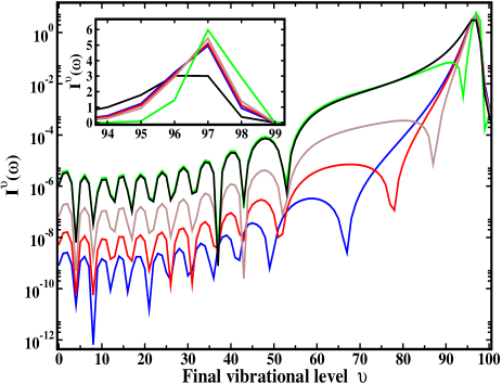
Figure 9: (Color online) Dependence of the squared dipole transition moments $\displaystyle I^{v}(\omega)$ on the scattering length $a_{\rm sc}$ for transitions from the first trap-induced ($v^{\prime}=11$) initial $a^{3}\Sigma^{+}_{u}$ state to the vibrational manifold ($v$) of the $1^{3}\Sigma^{+}_{g}$ state of $\mbox{Li}_{2}$ in a $\displaystyle\omega=2\pi\times\mbox{100\,kHz}$ trap. Using masses slightly larger than the one of ⁶Li $\displaystyle a_{sc}=+50\,a_{0}$ (blue), $\displaystyle a_{sc}=+115\,a_{0}$ (red), $\displaystyle a_{sc}=+350\,a_{0}$ (brown), and $\displaystyle a_{sc}=+2020\,a_{0}$ (green) were yielded. For comparison, the result with the physical mass ($\displaystyle a_{sc}=-2030\,a_{0}$, black) is also shown. The insert shows the transitions to $v=94$ to 99 on an enlarged scale.

It should be emphasised that of course also for $a_{\rm sc}<0$ a number of dips occur as was discussed in the context of Fig. 4. The difference between those dips and the one discussed for $a_{\rm sc}\gg 0$ is the occurrence of the latter outside the molecular regime. While the other dips are a direct consequence of the short-range part of the atom-atom interaction potential and thus confined (for Li₂) to $v<55$ corresponding to $R<30\,a_{0}$, the dip occuring for $a_{\rm sc}\gg 0$ can be located outside the molecular regime. This is even more apparent from Fig. 9 where the $I^{v}$ spectra for four different positive values of $a_{\rm sc}$ are shown together with the one for the (physical) value $a_{\rm sc}=-2030\,a_{0}$ (all for $\omega=2\,\pi\times 100\,$kHz). The values $a_{\rm sc}=+2020\,a_{0}$, $+350\,a_{0}$, $+115\,a_{0}$, and $+50\,a_{0}$ were obtained by a mass increase of $\sim 0.3$%,$\sim 0.8$%,$\sim 2$%, and $\sim 6$%, respectively. In agreement with the explanation given above, the position of the dip moves continuously to larger values of $v$ as the scattering length increases, since the position $R_{\rm x}$ of the last node of the initial state lies close to $a_{\rm sc}$. Also the positions of the other dips depend on $a_{\rm sc}$, but their dependence is much weaker and involves a much smaller $R$ interval. Clearly, the positions of the dips become more stable if they occur at smaller $v$.

Noteworthy, the positions of the first 10 dips agree perfectly for $a_{\rm sc}=-2030$ and $+2020\,a_{0}$. In fact, both spectra are on a first glance in almost perfect overall agreement, except the occurrence of the additional dip for $v=92$. According to the discussion of the sum rule in Sec. III.2 the total sum $\tilde{I}$ should be (approximately) independent of the atomic interaction and thus $a_{\rm sc}$. This is also confirmed numerically for the present examples. The insert of Fig. 9 reveals how the sum-rule is fulfilled. The due to the additional dip missing transition probability is compensated by an enhanced rate to the neighbor states with larger $v$.

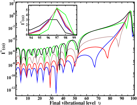
Figure 10: (Color online) As Fig. 9, but for a variation of $a_{\rm sc}$ by means of a reduction of the mass with respect to the one of ⁶Li. In this case, the number of bound states remains unchanged and the transition starts from the $v^{\prime}=10$ $a^{3}\Sigma^{+}_{u}$ state.

In all shown cases with $a_{\rm sc}>0$ there exist 11 bound states in contrast to the 10 states of ⁶Li ($a_{\rm sc}=-2030\,a_{0}$). As mentioned in the beginning of this section, it is also possible to change the sign of $a_{\rm sc}$ while preserving the number of nodes. The corresponding $I^{v}$ spectra (again for $\omega=2\pi\times 100\,$kHz) are shown in Fig. 10. The same values of $a_{\rm sc}$ as in Fig. 9 ($+2020\,a_{0}$, $+350\,a_{0}$, $+115\,a_{0}$, and $+50\,a_{0}$) are now obtained by a decrease of the mass by $\sim 18$%, $\sim 17.5$%, $\sim 16$%, and $\sim 13$%, respectively. A comparison of the two Figs. 9 and 10 demonstrates that the position of the outermost dip (for $a_{\rm sc}\gg 0$) depends for a given $\omega$ solely on $a_{\rm sc}$, while the other dips (in the molecular regime) differ when changing the total number of bound states from 10 to 11. A comparison of the results obtained for $a_{\rm sc}=-2030\,a_{0}$ and $+2020\,a_{0}$ with 10 bound states in both cases shows that most of the nodes in the molecular regime are shifted with respect to each other in such a way that the $v$ range hosting 10 dips for $a_{\rm sc}=-2030\,a_{0}$ contains 9 dips for $a_{\rm sc}=-2030\,a_{0}$.

Turning back to Fig. 7 and the question of the influence of a tight trap on the photoassociation rate for $a_{\rm sc}\gg 0$ one notices that the position of the additional dip appears to be practically independent of $\omega$. As was explained in the context of Fig. 8, the reason is that the position of the outermost node depends only weakly on $\omega$. For the shown example this shift is even for a 100 kHz trap small compared to the separation of the outermost lobes between neighboring $v$ states. Therefore, the shift is not sufficient to move the dip position away from $v=92$. However, if $a_{\rm sc}$ is, e. g.  increased to $+2020\,a_{0}$ the crossing point $R_{\rm x}$ shifts in a 100 kHz trap to about $1500\,a_{0}$ and changes thus by $\approx 25\,\%$. In this case the dip position moves from $v=95$ to $94$. It is therefore important to take the effects of a tight trap into account, if they are used for the determination of $a_{\rm sc}$ using photoassociation spectroscopy the way discussed in Côté et al. (1995); Abraham et al. (1996b).

In order to focus on the effect of the tight trap it is again of interest to consider the ratio $f^{v}(\omega)$ introduced in Sec. III.3. For small but positive values of $a_{\rm sc}$ the ratio $f^{v}$ is structurally very similar to the case $a_{\rm sc}=-2030\,a_{0}$ shown in Fig. 4 (b). A uniform constant regime covering almost all $v$ states is followed by a sharp cut-off whose position shifts to smaller $v$ as $\omega$ increases. A similar behavior is encountered for $a_{\rm sc}=+850\,a_{0}$ and $\omega=10\,$kHz as shown in Fig. 7 (b). However, for a tighter trap (100 kHz) a new feature appears. In this case the relative enhancement at the dip position ($v=92$) is smaller than in the constant regime, but larger for the neighbor states. The enhancement factor for $v=92$ is only $\approx 25\,\%$ of $f_{c}$, while the one for $v=93$ is $\approx 60\,\%$ larger than $f_{c}$. This results in a dispersion-like structure in $f^{v}$. It should be emphasised that this is again remarkably different from the other dips in $I^{v}(\omega)$ ($v<55$) that show the same (constant) enhancement factor $f_{c}$ as their neighbor states.

III.7 Combined influence of trap and atomic interaction

In view of the very important question how the efficiency of photoassociation can be improved, Fig. 9 reveals that besides the use of a tight trap a large scattering length is also favorable. The photoassociation rate (away from the dips) is enhanced by orders of magnitude, if $a_{\rm sc}$ varies from $a_{\rm sc}=+50\,a_{0}$ to $a_{\rm sc}=+2020\,a_{0}$! In view of the already discussed fact that the results for the overall spectrum $I^{v}$ differ for $a_{\rm sc}>0$ and $a_{\rm sc}<0$ only by the position of the dips, it is evident that photoassociation (or corresponding Raman transitions) are much more efficient, if $|a_{\rm sc}|$ is very large.

In order to understand the dependence of the FC factors of the vibrational final states on the scattering length it is instructive to look at the variation of the initial-state wave function with $a_{\rm sc}$ for large $R$ values. This is shown in Fig. 11 for $\displaystyle\omega=2\pi\times\mbox{100\,kHz}$.

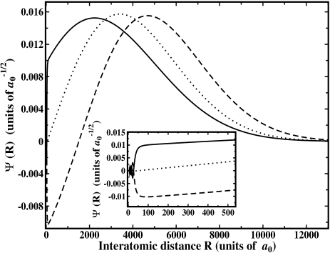
Figure 11: Wave functions of the initial state describing two Li atoms in a trap with frequency $\displaystyle\omega=2\pi\times 100\,\mbox{kHz}$ for different masses that yield the scattering lengths $a_{\rm sc}=-2030\,a_{0}$ (solid), $a_{\rm sc}=+50\,a_{0}$ (dots), and $a_{\rm sc}=+2020\,a_{0}$ (dashes). The insert shows the small $R$ range on an enlarged scale.

While a large attractive interaction ($a_{\rm sc}\ll 0$) leads to a very confined wave function for the first trap-induced bound state, a large repulsive interaction ($a_{\rm sc}\gg 0$) does not only result in a node (responsible for the photoassociation window discussed above), but also to a push of the outermost lobe to larger $R$ values. This push is of course counteracted by the confinement of the trap. However, only the highest lying final states probe the very large $R$ range. As is apparent from Fig. 2 the final states $v\leq 92$ probe almost completely the range $R\leq 1000\,a_{0}$. Within this $R$ interval the absolute value of the initial-state wave function increases with the absolute value of $a_{\rm sc}$. As a consequence, the corresponding FC factors and $I^{v}$ should increase with $|a_{\rm sc}|$. An exception to this is the already discussed occurrence of the photoassociation window (spectral dip) that occurs for a positive scattering length, if the position of the node is probed by the final-state wave function. Consequently, one expects for the low-lying final states (in fact for almost all except the very high-lying ones and the ones at the dip position) that an increase of $|a_{\rm sc}|$ leads to an increased photoassociation rate.

An evident question is of course, whether the enhancements due to the use of tighter traps and tuning of $a_{\rm sc}$ can be used in a constructive fashion? In order to investigate this question, one can introduce another enhancement factor

$$g^{v}(\omega,a_{\rm sc})\;=\;\frac{I^{v}(\omega,a_{\rm sc})}{I^{v}(\omega_{\rm ref},a_{\rm sc,ref})}$$ (7)

with $a_{\rm sc,ref}=0\,a_{0}$ (and $\omega_{\rm ref}=2\pi\times 1\,$kHz as before). Clearly, a cut through $g^{v}(\omega,a_{\rm sc})$ for constant $a_{\rm sc}$ is equal to $f^{v}(\omega)$. A cut for constant $\omega$ describes on the other hand the relative enhancement of the photoassociation rate as a function of $a_{\rm sc}$.

The function $g^{v}(\omega,a_{\rm sc})$ depends of course on the vibrational state $v$, but as was discussed before, most of the states show a constant enhancement factor $f_{c}$. Thus it is most interestingly to investigate $g_{c}(\omega,a_{\rm sc})$ that is defined as the $g$ function for vibrational states for which the relation $f^{v}=f_{c}$ is valid. This excludes the states in the cut-off regime and those at or very close to the photoassociation window.

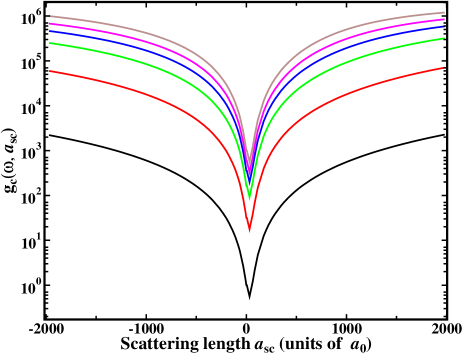
Figure 12: (Color online) Enhancement factor $g_{c}$ [see Eq. (7)] in the constant ($v$-independent) regime as a function of $a_{\rm sc}$ for trap frequencies $\omega=2\pi\times 1\,$kHz (black), $\omega=2\pi\times 10\,$kHz (red), $\omega=2\pi\times 30\,$kHz (green), $\omega=2\pi\times 50\,$kHz (blue), $\omega=2\pi\times 70\,$kHz (purple), and $\omega=2\pi\times 100\,$kHz (brown).

In Fig. 12 $g_{c}(\omega,a_{\rm sc})$ is shown as a function of $a_{\rm sc}$ for different trap frequencies. The important finding is that $g_{c}(\omega,a_{\rm sc})$ increases as a function of $\omega$ and $|a_{\rm sc}|$. In fact, within the shown ranges of $\omega$ and $a_{\rm sc}$ the function $g_{c}(\omega,a_{\rm sc})$ raises by 6 orders of magnitude, if the maximum values of $\omega$ ($2\pi\times 100\,$kHz) and $a_{\rm sc}$ ($\pm 2000\,a_{0}$) are considered! A more detailed analysis shows that the enhancement is almost equally distributed among the two parameters, i. e. a factor 10³ stems from the variation of $\omega$ and about the same factor from varying $a_{\rm sc}$. Thus the enhancement of the photoassociation rate due to the two different physical parameters occurs practically independently of each other, at least in the rather large parameter range considered. It should be emphasized that these ranges are realistically achievable in present-day experiments. It is interesting to note that this finding is not only very encouraging with respect to the possible enhancement of photoassociation rates and related molecule production schemes, but it shows also that the influence of the parameters scattering ($a_{\rm sc}$) and characteristic length scale of an isotropic harmonic trap ($\displaystyle a_{\rm ho}=\sqrt{1/(\mu\omega)}$) on the photoassociation process is very different from the one observed for the energy. In energy-related discussions (like the one on the validity of the pseudopotential approximation in Blume and Greene (2002)) it was found that the ratio $\displaystyle|a_{\rm sc}/a_{\rm ho}|$ determines the behavior. In the present case, both parameters and not only their ratio are important.

IV Pseudopotential approximation

The bound state of two atoms in a harmonic trap when the atom-atom interaction $V_{\rm int}(R)$ is approximated by a regularized contact potential $\displaystyle\frac{4\pi}{2\mu}a_{\rm sc}\delta^{3}(\vec{R})\frac{\partial}{\partial R}\,R$ with energy-independent scattering length $\displaystyle a_{\rm sc}$, was first derived analytically by Busch at al. Busch et al. (1998). The bound states with integer quantum number $\displaystyle n_{t}$ are expressed as

$$\Psi^{n_{t}}_{a_{\rm sc}}(R)=\frac{1}{2}\pi^{-3/2}ARe^{-\bar{R}^{2}/2}\Gamma(-\nu)U(-\nu,\frac{3}{2},\bar{R}^{2})\;,$$ (8)

with $\bar{R}=R/a_{\rm ho}$ and the characteristic length scale $a_{\rm ho}$ of the harmonic trap introduced in the end of the previous section. $\displaystyle A$ is a normalization constant having the dimension of the inverse of the square root of volume (see below) and $\nu$ is an effective quantum number for the relative motional eigenstate, $\displaystyle\nu=\frac{E_{a_{\rm sc}}^{n_{t}}}{2\omega}-\frac{3}{4}$. The energy eigenvalues are given by the roots of the equation

$$\frac{\Gamma(-x/2+3/4)}{\Gamma(-x/2+1/4)}=\frac{1}{\sqrt{2}\xi}\;,$$ (9)

where $x=E_{a_{\rm sc}}^{n_{t}}/\omega$ and $\xi=a_{\rm sc}/a_{\rm ho}$.

The initial-state wave function $\Psi^{\rm 10^{\prime}}(R;\omega)$ of two ${}^{6}\mbox{Li}$ atoms interacting through the $a^{3}\Sigma^{+}_{u}$ potential and the pseudopotential wave function $\displaystyle\Psi_{a_{\rm sc}}^{0}$ with the physical (trap-free) value of the scattering length $\displaystyle a_{\rm sc}=-2030\,a_{0}$ are plotted together in Fig. 13 for the case of a trap frequency $\displaystyle\omega=2\pi\times\mbox{10kHz}$.

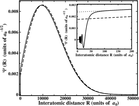
Figure 13: Wave functions of the first trap-induced bound state ($\displaystyle\omega=2\pi\times\mbox{10kHz}$) of two ${}^{6}\mbox{Li}$ atoms interacting through the full $a^{3}\Sigma^{+}_{u}$ potential (solid), a pseudopotential with the energy-independent (trap-free) scattering length $\displaystyle a_{\rm sc}=-2030\,a_{0}$ (dashes), and one with the energy-dependent value $\displaystyle a_{E}=-2872\,a_{0}$ (dots). The insert shows the short $R$ range on an enlarged scale.

As expected, wave function $\displaystyle\Psi_{a_{\rm sc}}^{0}$ fails completely for short internuclear separations, since it does not reproduce any nodal structure at all. In addition, $\displaystyle\Psi_{a_{\rm sc}}^{0}$ possesses a wrong behavior at $R=0$ where it is non-zero. In the long-range part $\displaystyle\Psi_{a_{\rm sc}}^{0}$ agrees better with the correct wave function. There the main difference is an evident phase shift between the two functions. This phase shift is a consequence of the trap and vanishes in the absence of the trap ($\omega\rightarrow 0$). The physical reason for the phase shift is the non-zero ground-state energy in a trap (zero-point energy and motion) due to the Heisenberg uncertainty principle. As a consequence, the scattering of the two atoms in a trap differs from the trap-free case even at zero temperature. On the basis of an analysis of the energy spectrum of two atoms in a harmonic trap it was found that a pseudopotential approximation using an energy-dependent scattering length $\displaystyle a_{E}$ leads to a highly improved description of two particles confined in an isotropic harmonic trap Blume and Greene (2002); Bolda et al. (2003).

While the scattering length is defined in the limit $E\rightarrow 0$, an energy-dependent scattering length can be introduced by extending its original asymptotic definition in terms of the phase shift for s-wave scattering $\delta_{0}(E)$ to non-zero collision energies. This yields $\displaystyle a_{E}=-\mbox{tan}\delta_{0}(E)/k$ with $\displaystyle k=\sqrt{2\mu E}$. Clearly, the evaluation of $\delta_{0}(E)$ requires to solve the complete scattering problem and thus also $\displaystyle a_{E}$ can only be obtained from the knowledge of the solution for the correct atom-atom interaction potential.

The values of $\displaystyle a_{E}$ were obtained in the following way. After a determination of the ground-state energy of two ${}^{6}\mbox{Li}$ atoms from a full calculation (using the realistic interaction potential), this energy is used in Eq. (9) to find $\displaystyle a_{E}$ (that is inserted in the equation in place of $\displaystyle a_{\rm sc}$). More details about this so-called self-consistency approach are given in Bolda et al. (2002). In this way an energy-dependent scattering length $\displaystyle a_{E}=-2872\,a_{0}$ is, e. g., found for two ⁶Li atoms in a trap with frequency $\displaystyle\omega=2\pi\times\mbox{10kHz}$. The resulting wave function is also shown in Fig. 13, together with the correct one and the one obtained for $\displaystyle a_{\rm sc}=-2030\,a_{0}$. Clearly, the agreement with the correct wave function is very good for large $R$. For $R>150\,a_{0}$ the wave function obtained for $\displaystyle a_{E}=-2872\,a_{0}$ is not distinguishable from the correct one. Only in the insert of Fig. 13 that shows the wave functions at short internuclear separations one sees a deviation. It is caused by the absence of any nodal structure and the wrong behavior at $R\rightarrow 0$ of the pseudopotential wave function. In fact, at short distances the introduction of an energy-dependent scattering length that corrects the phase shift leads to an even larger error compared to the use of $a_{\rm sc}$.

The validity of the pseudopotential approximation using an energy-dependent scattering length has been discussed before. In Blume and Greene (2002) it was found that applicability of this approximation depends on the ratios $\displaystyle\beta_{6}/a_{\rm ho}$ and $\displaystyle|a_{\rm sc}/a_{\rm ho}|$ where $\displaystyle\beta_{6}=(2\mu C_{6})^{1/4}$ is the characteristic length scale of the interaction potential in the case of a leading $C_{6}/R^{6}$ van der Waals potential. For two ${}^{6}\mbox{Li}$ atoms in a trap with $\displaystyle\omega=2\pi\times\mbox{100\,kHz}$ that interact via the $\displaystyle a^{3}\Sigma^{+}_{u}$ potential those ratios are 0.02 and 0.59, respectively. These validity criteria are, however, based solely on energy arguments. In other words, if those ratios are sufficiently smaller than 1, the energy obtained by means of Eq. (9) with $a_{\rm sc}$ should agree well with the correct one. In the present example of ${}^{6}\mbox{Li}$ the ratio between the correct first trap-induced energy $E^{10^{\prime}}$ and $E^{n_{t}=0}_{a_{\rm sc}}$ obtained with the energy-independent pseudopotential is $E^{10^{\prime}}/E^{0}_{a_{\rm sc}}=0.96$ for $\displaystyle\omega=2\pi\times\mbox{10\,kHz}$ and $E^{10^{\prime}}/E^{0}_{a_{\rm sc}}=0.92$ for $\displaystyle\omega=2\pi\times\mbox{100\,kHz}$. By construction, the energy $E^{n_{t}0}_{a_{\rm E}}$ agrees of course completely with $E^{10^{\prime}}$.

In Fig. 14 $I^{v}(\omega)$ obtained when using the pseudopotential approximation with energy-independent scattering length is compared to the spectrum obtained for the correct atom-atom interaction, both for a trap frequency $\displaystyle\omega=2\pi\times\mbox{10\,kHz}$.

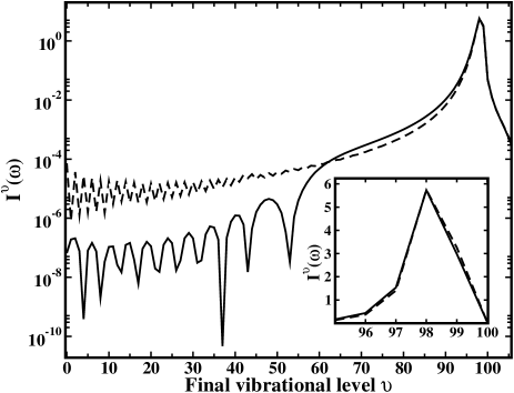
Figure 14: Squared photoassociation transition moments $\displaystyle I^{v}(\omega)$ for ⁶Li in a $\omega=2\pi\times 10\mbox{\,kHz}$ trap calculated with the molecular interaction potential (solid) or within the energy-independent pseudopotential approximation (dashes).

The two results disagree completely for $v\leq 60$. For higher lying vibrational states ($v>60$) the agreement is reasonable. (Note, however, the logarithmic scale.) For the highest lying states ($v\geq 95$) very good agreement is found even on a linear scale (see insert of Fig. 14). Adopting the energy-dependent scattering length yields quantitative agreement already for $v\geq 75$, but again a complete disagreement for $v\leq 60$.

The breakdown of the pseudopotential approximation (with energy-independent or dependent scattering length) for describing photoassociation to the low-lying vibrational states is, of course, a direct consequence of the wrong short-range behavior of the pseudopotential wave functions (Fig. 13). From the definition of $I^{v}(\omega)$ it follows that the pseudopotential approximation fails, if the final-state vibrational wave function has a substantial amplitude in the $R$ range in which the initial-state wave function is strongly influenced by the atom-atom interaction. An estimate for this $R$ range is (in the present case) the already discussed effective-range parameter $\displaystyle\beta_{6}=(2\mu C_{6})^{1/4}$. Since for large $v$ the final-state wave function is dominated by its outermost lobe whose position is in turn close to the classical outer turning point $R_{\rm out}$, the pseudopotential approximation should be valid for $\displaystyle R_{\rm out}>\beta_{6}$. In the case of ⁶Li one finds $\beta_{6}=62.5\,a_{0}$. According to Fig. 2 the pseudopotential approximation should thus be applicable for $v>70$. A recently performed photoassociation experiment for ${}^{6}\mbox{Li}$ considered the transition to $\displaystyle v=59$ Schloeder et al. (2003). For this specific example the pseudopotential approximation would predict a two times smaller rate than the full calculation for $\displaystyle\omega=2\pi\times\mbox{10\,kHz}$.

The validity of the pseudopotential approximation for predicting the photoassociation rates to the high lying states can also be used to investigate whether the simulation of different scattering lengths by mass scaling is senseful. This could be questionable, since a change of the mass does not only modify the scattering length (by moving the position of the least bound state), but also the kinetic energy term. Thus it may be argued that the discussed influence of the scattering length on the photoassociation process could partly also be a consequence of the modification of the kinetic energy, at least in the case of a substantial mass variation as it was required for preserving the number of bound states. Within the pseudopotential approximation the scattering length is, however, a parameter independent of the mass. Therefore, in contrast to the case of the full calculation it is possible within the pseudopotential approximation to investigate the isolated influence of a variation of the scattering length (keeping the mass fixed). A corresponding analysis confirms that mass scaling can in fact be used to simulate a modified atom-atom interaction.

The pseudopotential approximation was used already in Deb and You (2003) for an analysis of the change of the photoassociation rate due to a scattering-length modification. The investigation concentrated, however, on very high lying vibrational states close to or even above the trap-free dissociation limit. Since for transitions to those states the $R$ dependence of the electronic transition dipole moment can safely be ignored, it is sufficient to concentrate on the Franck-Condon (FC) factors. In Fig. 15 the squares of these factors are shown as a function of the scattering length for $90\leq v\leq 98$ and trap frequency $\displaystyle\omega=2\pi\times\mbox{100\,kHz}$.

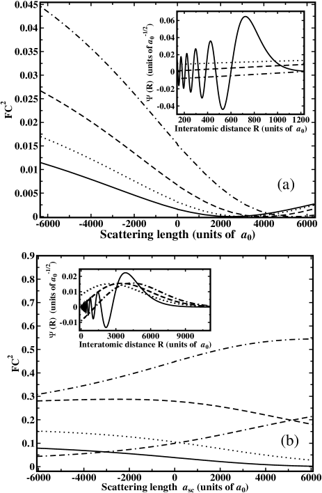
Figure 15: (a) Squared Franck-Condon factors between the final vibrational states $v=90$ (solid), 91 (dots), 92 (dashes), or 93 (chain) of the $1^{3}\Sigma^{+}_{g}$ state and the initial-state pseudopotential wave functions as a function of the scattering length $a_{\rm sc}$. The trap frequency is $\displaystyle\omega=2\pi\times\mbox{100\,kHz}$. The insert shows the $v=92$ final-state wave function together with the pseudopotential wavefunctions for $a_{sc}=-2000\,a_{0}$ (dots), $a_{sc}=0$ (dashes), $a_{sc}=+2000\,a_{0}$ (chain). (b) As (a), but for $v=94$ (solid), 95 (dots), 96 (dashes), 97 (chain), v=98 (dot-dash-dash). The insert shows the $v=97$ final-state wavefunction and the pseudopotential wave functions for $a_{sc}=-2000\,a_{0}$ (dots), $a_{sc}=0$ (dashes), $a_{sc}=+2000\,a_{0}$ (chain).

As in Deb and You (2003) the pseudopotential approximation is used for the initial state, but here the final-state wave function is obtained by a full numerical calculation while an approach based on quantum defect theory (QDT) was used in Deb and You (2003). Furthermore, Na₂ was considered in Deb and You (2003) while it is Li₂ in the present study.

For the states $90\leq v\leq 93$ shown in Fig. 15(a) the dependence on $a_{\rm sc}$ in a 100 kHz trap is very similar to the one found in Deb and You (2003). The rather regular variation with $a_{\rm sc}$ is due to the fact that the final-state wave function probes the flat part of the initial-state wave function, as can be seen in the insert of Fig. 15(a) where the wave function for $v=92$ is shown together with the initial-state wave function for three different values of $a_{\rm sc}$. The initial-state wave function varies almost linearly with $a_{\rm sc}$ in the Franck-Condon window of the $v=92$ final state. According to the discussion in Sec. III.5, for a 100 kHz trap the states $v\geq 90$ belong to the cut-off regime, but for $v\leq 93$ the enhancement factor $f^{v}$ is still close to its value $f_{c}$ in the constant regime (see Figs. 4 and 7). The minima of the FC² factors for $a_{\rm sc}\gg 0$ are a consequence of the dip discussed in Sec. III.6. Since the nodal position $R_{\rm x}$ moves to larger $R$ if $a_{\rm sc}$ increases, the minimum in the FC² factors moves to a larger value of $a_{\rm sc}$ if $v$ increases. While the pseudopotential approximation is capable to predict the existence of the dip occuring for $a_{\rm sc}\gg 0$, its position is not necessarily correctly reproduced in a trap. This is due to the fact that the pseudopotential overestimates the trap-induced shift of the position of the outermost node. For example, if the mass of Li is varied such that $a_{\rm sc}=+850\,a_{0}$ is obtained, a 100 kHz trap shifts $R_{\rm x}$ to $\approx+810\,a_{0}$ (Fig. 8) and the dip occurs at $v=92$ (Fig. 7). Using the pseudopotential approximation (with $a_{\rm sc}=+850\,a_{0}$) yields on the other hand $R_{\rm x}\approx+580\,a_{0}$ and the dip occurs for $v=90$. This error in the prediction of $R_{\rm x}$ increases with $a_{\rm sc}$.

The final states $94\leq v\leq 98$ whose FC² factors are shown in Fig. 15(b) probe on the other hand the non-linear part of the initial-state wave function (close to the trap boundary). Consequently, the dependence on $a_{\rm sc}$ differs from the one found in Deb and You (2003). While for $90\leq v\leq 92$ the FC² factors are first decreasing and then increasing, if $a_{\rm sc}$ varies from $-6000\,a_{0}$ to $+6000\,a_{0}$, the ones of $93\leq v\leq 96$ are purely decreasing. For $v=97$ and 98 the FC² factors are on the other hand increasing with $a_{\rm sc}$.

In view of the fact that the scattering length of a given atom pair may be known (for example from some measurement), but the corresponding atom-atom interaction potential is unknown, it is of course interesting to investigate whether the pseudopotential approximation allows to predict the enhancement factor also in the constant regime, i. e. whether it correctly reproduces $f_{c}(\omega)$. This would allow for a simple estimate of the effect of a tight trap on the photoassociation rate in the constant regime that covers most of the spectrum. In order to determine $f_{c}(\omega)$ it is sufficient to analyze the ratio of the initial-state wave function $\Psi_{a_{\rm sc}}^{0}$ for the trap frequencies $\omega$ and $\omega_{\rm ref}$. This comparison may be done at any arbitrary internuclear separation $R_{\rm lin}$ provided it belongs to the linear regime. The result is

$$\displaystyle f_{c}^{\rm pseudo}({\omega})=\left[\frac{\Psi^{0}_{a_{\rm sc}}(R_{\rm lin};\omega)}{\Psi^{0}_{a_{\rm sc}}(R_{\rm lin};\omega_{\rm ref})}\right]^{2}\;.$$ (10)

A very special and simple choice that guarantees that $R_{\rm lin}$ belongs to the linear regime is $R_{\rm lin}=0$. With this value of $R_{\rm lin}$ one finds from the analysis of $\Psi^{0}_{a_{\rm sc}}$

$$\displaystyle f_{c}^{\rm pseudo}({\omega})=\left[\frac{A({\omega})}{A({\omega_{\rm ref}})}\right]^{2}\>\frac{\omega_{\rm ref}}{\omega}\;,$$ (11)

where $\displaystyle A({\omega})$ is the normalization factor fulfilling $\displaystyle|A({\omega})|^{2}\,=\,\sqrt{2\omega}\,\pi\,\xi^{2}\,\frac{\partial E}{\partial\xi}$ Busch et al. (1998). Depending on the level of approximation one may use either $a_{\rm sc}$ or $a_{E}$ in the evaluation of $A$. An even simpler estimate of the influence of a tight harmonic trap on the photoassociation rate is obtained, if the atom-atom interaction potential is completely ignored in the initial state. The harmonic-oscillator eigenfunctions at $R=R_{\rm lin}=0$ yield

$$f_{c}^{\rm ho}({\omega})=\left(\,\frac{\omega}{\omega_{\rm ref}}\right)^{3/2}\;.$$ (12)

In Fig. 16 the enhancement factors $f_{c}(\omega)$ calculated at the different levels of approximation are shown as a function of the trap frequency $\omega$.

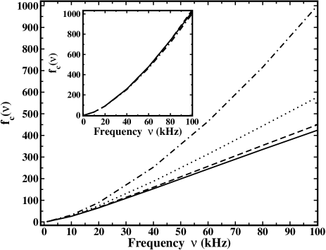
Figure 16: Dependence of the enhancement factor $\displaystyle f_{c}$ on the trap frequency $\nu=\omega/(2\pi)$ for ${}^{6}\mbox{Li}_{2}$ using the molecular (solid), the energy-independent (dots) and -dependent (dashes) pseudopotential, or the harmonic-oscillator (chain) wave functions. The insert shows the same curves but for ³⁹K₂.

The results obtained for ⁶Li and ³⁹K are compared to each other. Remind, in the latter case the scattering length $a_{\rm sc}=+90\,a_{0}$ has a much smaller absolute value than for ⁶Li ($a_{\rm sc}=-2030\,a_{0}$). Consequently, one expects the atom-atom interaction to be less important. This is confirmed by (the insert of) Fig. 16. The results obtained for $f_{c}(\omega)$ with the aid of the different approximations discussed above are in very good agreement with the correct result in the case of ³⁹K. Even the simple harmonic-oscillator model predicts the enhancement factor in the constant regime very accurately.

It should be emphasized that the correct prediction of the enhancement factor by the simplified approximation works, although the prediction of the rates is completely wrong (Fig. 14) in this constant regime (small $v$). In the case of a large absolute value of the scattering length (like for ⁶Li), i. e. for a strong atom-atom interaction, the frequency dependence of $f_{c}(\omega)$ predicted by the simplified models is on the other hand not very accurate. In fact, the simple harmonic-oscillator model clearly overestimates the enhancement factor for large $\omega$. The pseudopotential approximation yields much better results, especially if the energy-dependent scattering length $a_{E}$ is used. (As already mentioned, $a_{E}$ is, however, only available from the knowledge of the exact atom-atom interaction.)

In view of the usefulness of Eq. (11) for obtaining an estimate of the enhancement factor $f_{c}(\omega)$ but the rather complicated procedure to calculate $\displaystyle\frac{\partial E}{\partial\xi}$ required for obtaining $\displaystyle A({\omega})$, it is interesting to test whether $\displaystyle A({\omega})$ can alternatively be evaluated from an expansion of the energy $\displaystyle E$ at $\displaystyle\xi=0$. Using the relation $\displaystyle\frac{\partial x}{\partial\xi}=\left(\frac{\partial\xi}{\partial x}\right)^{-1}$ it is straightforward to determine with the aid of (9) an expansion for the scaled energy

$$x(\xi)=\frac{3}{2}+\sum\limits_{n=0}^{\infty}\frac{1}{(n+1)!}\left.\frac{\partial^{(n)}F(x)}{\partial x^{(n)}}\right|_{x=3/2}\xi^{n+1}\,$$ (13)

with

$$F(x)=-\frac{2\sqrt{2}\,\Gamma\Bigl{[}\frac{3}{4}-\frac{x}{2}\Bigr{]}}{\Gamma\Bigl{[}\frac{1}{4}-\frac{x}{2}\Bigr{]}\psi\Bigl{[}\frac{1}{4}-\frac{x}{2}\Bigr{]}-\psi\Bigl{[}\frac{3}{4}-\frac{x}{2}\Bigr{]}}\,$$ (14)

and the digamma function $\psi$. The zero- and first-order terms of the expansion (13) are given in Busch et al. (1998). Using Eqs. (13) and (11)

$$f_{c}^{\rm pseudo}({\omega})=\frac{\sum\limits_{n=0}^{\infty}\frac{1}{n!}\left.\frac{\partial^{(n)}F(x)}{\partial x^{(n)}}\right|_{x=3/2}\xi^{n}}{\sum\limits_{n=0}^{\infty}\frac{1}{n!}\left.\frac{\partial^{(n)}F(x)}{\partial x^{(n)}}\right|_{x=3/2}\xi^{n}_{\rm ref}}\Bigl{(}\frac{\omega}{\omega_{\rm ref}}\Bigr{)}^{\frac{3}{2}}$$ (15)

is obtained with $\displaystyle\xi_{\rm ref}=\frac{a_{\rm sc}}{a_{\rm ho,ref}}$. In Fig. 17 the 4th-, 5th-, and 6th-order expansions are compared to the results obtained with the non-approximated term (all for $a_{\rm sc}=-2030\,a_{0}$) and with the correct atom-atom interaction result.

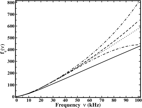
Figure 17: Investigation of the convergence of the series expansion (15) for the enhancement factor $\displaystyle f_{\rm c}^{\rm pseudo}(\omega)$ in the constant regime. Shown are the results of the full (infinite order, dotted) and the 4th (dashes), 5th (chain), and 6th (dot-dash-dash) order expansion. For comparison, also the enhancement factor obtained with the molecular potential is shown (solid).

Note, Eq. (15) can also be used for the evaluation of $g_{c}(\omega,a_{\rm sc})$, if in the denominator $\xi_{\rm ref}$ is replaced by $\displaystyle\tilde{\xi}_{\rm ref}=\frac{a_{\rm sc,ref}}{a_{\rm ho,ref}}$.

V Discussion and Outlook

In this work the influence of a tight isotropic harmonic trap on the photoassociation process has been investigated for alkali atoms. It is found that for most of the states (the ones in the constant regime) there is an identical enhancement as the trap frequency increases. This enhancement can reach 3 orders of magnitude for trap frequencies of about 100 kHz as they are reported in literature. While the enhancement itself agrees at least qualitatively with the concept of confinement of the initial-state wave function, also trap-induced suppressed photoassociation is possible. In fact, as a simple sum rule confirms, any enhancement must be accompanied by suppression. The physical origin of this suppression is the trap-induced confinement of the initial-state wave function of relative motion within a radius that is smaller than the mean internuclear separation of the least bound vibrational states in the electronic target state. Since in the present calculation both initial and final state are exposed to the same harmonic trap, this result may appear surprising. While the explanation is based on the different long-range behaviors of the two involved electronic states, the effect itself may be very interesting in terms of, e. g., quantum information.

Consider for example an optical lattice as trapping potential. The initial (unbound) atom pair is (for sufficient trap depths) located within a single lattice site (Mott insulator state). In the photoassociated state it could, however, reach into and thus communicate with the neighbor site, if the lattice parameters are appropriately chosen. Such a scenario could be used for a controlled logical operation (two-qubit gate) like the CNOT. Since the latter forms together with single-qubit gates a universal gate, this could provide a starting point for a quantum computer. Alternatively, it may be interesting to use the fact that if a single spot with the dimension of the trap length $a_{\rm ho}$ or a specific site in an optical lattice can be addressed, then the atoms would only respond, if they are in their (unbound) initial state. If they are in the photoassociated excited state, they would on the other hand be located outside the trap and thus would not respond. For this it is already sufficient, if they are (predominantly) located in the classically forbidden regime. Also, modifying the trap frequency it is possible to block the photoassociation process on demand. The trap frequency is then varied in such a fashion that a specific final state resonantly addressed with a laser with sufficiently small bandwidth belongs either to the constant or to the cut-off regime.

A further important finding of this work is that the influence of a tight trap on the photoassociation spectra (as a function of the final vibrational state) for different alkali atoms is structurally very similar, independent whether photoassociation starts from the singlet or triplet ground state. Also the type of interaction (strong or weak as well as repulsive or attractive) does not lead to a substantial modification of the trap influence. The only exception is a strong repulsive interaction that leads to a pronounced window in the photoassociation spectrum. The reason is the position of the last node in the initial-state wave function that in this case is located at a relatively large value of $R$ and leads to a cancellation effect in the overlap with the final state. The nodal position depends strongly on $a_{\rm sc}$, but only for very tight traps also on $\omega$. As has been discussed previously Côté and Dalgarno (1998); Abraham et al. (1996b), the position of the window may be used for a scattering-length determination. This will also approximately work for not too tight traps, but the trap influence has to be considered for very tight ones. Alternatively, the window provides a control facility, since the transition to a single state can be selectively suppressed. In very tight traps this effect is not only more pronounced, but in addition the transitions to the neighbor states are further enhanced. This could open up a new road to control in the context of the presently on-going discussion of using femtosecond lasers for creating non-stationary wave packets in the electronic excited state Salzmann et al. (2006); Brown et al. (2006); Koch et al. (2006). One of the problems encountered in this approach is the difficulty to shape the wave packet, since the high-lying vibrational states that have a reasonable transition rate are energetically very closely spaced and thus the shape of the wavepacket is determined by the Franck-Condon factors that cannot easily be manipulated but strongly increase as a function of $v$.

In view of the question how to enhance photoassociation or related association schemes (like Raman-based ones) the investigation of the enhancement factors $g^{v}(\omega,a_{\rm sc})$, especially its value in the constant regime ($g_{c}(\omega,a_{\rm sc})$) is most important. It shows that not only increasing the tightness of the trap (enlarging $\omega$) leads to an enhancement of the photoassociation rate, but a similar effect can be achieved by increasing the interaction strength $|a_{\rm sc}|$. Most interestingly, these two enhancement factors work practically independent of each other, i. e. it is possible to use both effects in a constructive fashion and to obtain a multiplicative overall enhancement factor. For a 100 kHz trap and a scattering length $|a_{\rm sc}|$ of the order of 2000 an enhancement factor (uniform for all states in the constant regime) of 5 to 6 orders of magnitude is found compared to the case of a shallow 1 kHz trap and $|a_{\rm sc}|=0$.

A comparison of the results obtained for the correct atom-atom interaction potential with the ones obtained using the approximate pseudopotential approximation or ignoring the interaction at all shows that these approximations yield only for the transitions to very high lying vibrational states a good estimate of the photoassociation rate. Nevertheless, despite the complete failure of predicting the rates to low lying states, these models allow to determine the enhancement factor in the constant regime. For weakly interacting atoms (small $|a_{\rm sc}|$) already the pure harmonic-oscillator model (ignoring the atomic interaction) leads to a reasonable prediction of the trap-induced enhancement factor $f_{c}(\omega)$.

It is important to stress that the results in this work were obtained for isotropic harmonic traps with the same trapping potential seen by both atoms. In this case center-of-mass and relative motion can be separated and in both coordinates an isotropic harmonic trap potential (with different trap lengths due to the different total and reduced masses) is encountered. As is discussed, e. g., in Bolda et al. (2003); Idziaszek and Calarco (2005) where a numerical and an analytical solution are respectively derived for the case of atoms interacting via a pseudopotential, a similar separation of center-of-mass and relative motion is possible for axially symmetric (cigar or pancake shaped) harmonic traps.

In reality, the traps for alkali atoms are of course not strictly harmonic. Since the present work focuses, however, for the initial atom pair on the lowest trap induced state the harmonic approximation should in most cases be well justified. Independently on the exact way the trap is formed (for example by a far off-resonant focused Gaussian laser beam or by an optical lattice), the lowest trap-induced state agrees usually well with the one obtained in the harmonic approximation, if the zero-point energy is sufficiently small. This requirement sets of course an upper scale to the applicability of the harmonic approximation with respect to the trap frequency. If $\omega$ is too large, the atom pair sees the anharmonic part of the trap. (Clearly, the trap potential must also be sufficiently deep to support trap-induced bound states, i. e. to allow for Mott insulator states in the case of an optical lattice).

An additional problem arises from the anharmonicity of a real trap: the anharmonic terms lead to a non-separability of the relative and the center-of-mass motion. In fact, a recent work discusses the possibility of using this coupling of the two motions for the creation of molecules Bolda et al. (2005). Again, a tighter trap is expected to lead to a stronger coupling and thus finally to a breakdown of the applicability of the harmonic model.

For the final state of the considered photoassociation process there exists on the first glance an even more severe complication. Usually, the two atoms will not feel the same trapping potential, since they populate different electronic states. In the case of traps whose action is related to the induced dipole moment (which is the case for optical potentials generated with the aid of lasers that are detuned from an atomic transition), the two atoms (in the case of Li the ones in the 2 ²S and the 2 ²P state) will in fact see potentials with opposite sign. If the laser traps the ground-state atoms, it repels the excited ones. In the alternative case of an extremely far-off resonant trap the trapping potential is proportional to the dynamic polarizability of the atoms. In the long-wavelength limit (as is realized, e. g., in focused CO₂ lasers Takekoshi et al. (1995)) the dynamic polarizability approaches the static one, $\lim_{\lambda\rightarrow\infty}\alpha(\lambda)=\alpha_{\rm st}$. The static polarizabilities do not necessarily have opposite signs for the ground and the excited electronic state of an alkali atom, but in many cases different values. Then the trapping potentials for the initial and final states of the photoassociation process are different. The Li system appears to be a counter example, since for ${}^{6}\mbox{Li}_{2}$ the average polarizability of the $a^{3}\Sigma^{+}_{u}$ (2s+2s) state is predicted to be equal to $\overline{\alpha}=\alpha_{zz}=\alpha_{xx}=2\alpha_{0}(2s)=2\times 165=330\,a_{0}$ For the $1^{3}\Sigma^{+}_{g}$ (2s+2$p_{z}$) state one has $\alpha_{zz}=\alpha_{0}(2s)+\alpha_{zz}(2p_{z})=285\,a_{0}$ and $\alpha_{xx}=\alpha_{0}(2s)+\alpha_{xx}(2p_{z})=292\,a_{0}$ yielding an average polarizability $\overline{\alpha}\approx 290\,a_{0}$ Mérawa and Rérat (2001). Thus the trapping potentials are expected to be very similar. This is not the case for, e. g., ⁸⁷Rb₂ where the average polarization for the $a^{3}\Sigma^{+}_{u}$ state is $670\,a_{0}$ and for $1^{3}\Sigma^{+}_{g}$ it is $1698\,a_{0}$ Magnier and Aubert-Frécon (2002).

It was checked that the use of very different values of $\omega$ for determining the initial and final state wave functions does not influence the basic findings of the present work. The reason is simple. Besides the very least bound states (and of course the trap-induced ones) the final states are effectively protected by the long-range interatomic potential from seeing the trap. However, if the two atoms are exposed to different trap potentials, a separation of center-of-mass and relative motion is again not possible, even in the fully harmonic case (a fact that was, e. g., overlooked in Koch et al. (2005)). One would again expect that this coupling increases with the difference in the trap potentials of the two involved states. A detailed study of the consequences of the coupling of center-of-mass and relative motion due to various reasons like an anharmonicity of the trap or different trapping potentials seen by the involved atoms is presently underway. This involves also the case of the formation of heteronuclear alkali dimers where besides the occurrence of this coupling for the initial state also a different long-range behavior of the interatomic potential has to be considered.

Different interaction strengths occur naturally for different alkali atoms as is well known and also evident from the explicit examples of ⁶Li, ⁷Li, and ³⁹K that were discussed in this work. According to the findings of this work the choice of a proper atom pair (with large $|a_{\rm sc}|$) enhances the achievable photoassociation yield quite dramatically. Clearly, for practical reasons it is usually not easy to change in an existing experiment the atomic species, since the trap and cooling lasers are adapted to a specific one. In addition, the naturally existing alkali species provide only a fixed and limited number of interaction strengths.

The tunability of the interaction strength on the basis of Feshbach resonances, especially magnetic ones, marked a very important corner-stone in the research area of ultracold atomic gases. The findings of the present work strongly suggest that this tunability could be used to improve the efficiency of photoassociation (and related) schemes. However, it has to be emphasized that it is not at all self-evident that the independence of the scattering-length variation and the one of the trap frequency as it occurs in the model used in this work is applicable to (magnetic) Feshbach resonances. Furthermore, the present work considered only the single-channel case while the proper description of a magnetic Feshbach resonance requires a multi-channel treatment. Noteworthy, a strong enhancement of the photoassociation rate by at least 2 orders of magnitude while scanning over a magnetic Feshbach resonance was predicted on the basis of a multichannel calculation for a specific ⁸⁵Rb resonance already in van Abeelen et al. (1998). An experimental confirmation followed very shortly thereafter Courteille et al. (1998). The explanation for the enhancement given in van Abeelen et al. (1998) is, however, based on an increased admixture of bound-state contribution to the initial continuum state in the vicinity of the resonance. This is evidently different from the reason for the enhancement due to large values of $|a_{\rm sc}|$ discussed in the present work.

An extension within the multichannel formalism that allows for a full treatment of magnetic Feshbach resonances is presently underway.

References

- Anderson et al. (1995) M. H. Anderson, J. R. Ensher, M. R. Matthews, C. E. Wieman, and E. A. Cornell, Science 269, 198 (1995).
- Jochim et al. (2003) S. Jochim, M. Bartenstein, A. Altmeyer, G. Hendl, S. Riedl, C. Chin, J. Hecker Denschlag, R. Grimm, C. Zhu, A. Dalgarno, et al., Science 302, 2101 (2003).
- Regal et al. (2003) C. A. Regal, C. Ticknor, J. L. Bohn, and D. S. Jin, Nature 424, 3 (2003).
- Zwierlein et al. (2003) M. W. Zwierlein, C. A. Stan, C. H. Schunck, S. M. F. Raupach, S. Gupta, Z. Hadzibabic, and W. Ketterle, Phys. Rev. Lett. 91, 250401 (2003).
- Lett et al. (1993) P. D. Lett, K. Helmerson, W. D. Phillips, L. P. Ratliff, S. L. Rolston, and M. E. Wagshul, Phys. Rev. Lett. 71, 2200 (1993).
- Fioretti et al. (1998) A. Fioretti, D. Comparat, A. Crubellier, O. Dulieu, F. Masnou-Seeuws, and P.Pillet, Phys. Rev. Lett. 80, 4402 (1998).
- Drummond et al. (2002) P. D. Drummond, K. V. Kheruntsyan, D. J. Heinzen, and R. H. Wynar, Phys. Rev. A 65, 063619 (2002).
- Abraham et al. (1995) E. R. I. Abraham, W. I. McAlexander, C. A. Sackett, and R. G. Hulet, Phys. Rev. A 74, 1315 (1995).
- Tiemann et al. (1996) E. Tiemann, H. Kn ckel, and H. Richling, Eur. Phys. J. D 37, 323 (1996).
- Fioretti et al. (2001) A. Fioretti, C. Amiot, C. Dion, O. Dulieu, M. Mazzoni, G. Smirne, and C. Gabbanini, Eur. Phys. J. D 15, 189 (2001).
- Gutterres et al. (2002) R. Gutterres, C. Amiot, A. Fioretti, C. Gabbanini, M. Mazzoni, and O. Dulieu, Phys. Rev. A 66, 024502 (2002).
- Schloeder et al. (2003) U. Schloeder, T. Deuschle, C. Silber, and C. Zimmermann, Phys. Rev. A 68, 051403 (2003).
- Jaksch et al. (2002) D. Jaksch, V. Venturi, J. I. Cirac, C. J. Williams, and P. Zoller, Phys. Rev. Lett. 89, 040402 (2002).
- Bolda et al. (2005) E. L. Bolda, E. Tiesinga, and P. S. Julienne, Phys. Rev. A 71, 033404 (2005).
- Koch et al. (2005) C. P. Koch, F. Masnou-Seeuws, and R. Kosloff, Phys. Rev. Lett. 94, 193001 (2005).
- Greiner et al. (2002) M. Greiner, O. Mandel, T. Esslinger, T. Hänsch, and I. Bloch, Nature 415, 39 (2002).
- Rom et al. (2004) T. Rom, T. Best, O. Mandel, A. Widera, M. Greiner, T. W. Hänsch, and I. Bloch, Phys. Rev. Lett. 93, 073002 (2004).
- Busch et al. (1998) T. Busch, B.-G. Englert, K. Rzazewski, and M. Wilkens, Found. of Phys. 28, 549 (1998).
- Idziaszek and Calarco (2005) Z. Idziaszek and T. Calarco, Phys. Rev. A 71, 050701 (2005).
- Blume and Greene (2002) D. Blume and C. H. Greene, Phys. Rev. A 65, 043613 (2002).
- Deb and You (2003) B. Deb and L. You, Phys. Rev. A 68, 033408 (2003).
- Almazor et al. (1999) M.-L. Almazor, O. Dulieu, M. Elbs, E. Tiemann, and F. Masnou-Seeuws, Eur. Phys. J. D 5, 237 (1999).
- Almazor et al. (2001) M.-L. Almazor, O. Dulieu, F. Masnou-Seeuws, R. Beuc, and G. Pichler, Eur. Phys. J. D 15, 355 (2001).
- Kemmann et al. (2004) M. Kemmann, I. Mistrik, S. Nussmann, and H. Helm, Phys. Rev. A 69, 022715 (2004).
- Colavecchia et al. (2003) F. D. Colavecchia, J. P. Burke, W. J. Stevens, M. R. Salazar, G. A. Parker, and R. T. Pack, J. Chem. Phys. 118, 5484 (2003).
- Linton et al. (1989) C. Linton, T. Murphy, F. Martin, R. Bacis, and J. Verges, J. Chem. Phys. 91, 6036 (1989).
- Schmidt-Mink et al. (1985) I. Schmidt-Mink, W. Müller, and W. Meyer, Chem. Phys. 92, 263 (1985).
- Marinescu and Dalgarno (1995) M. Marinescu and A. Dalgarno, Phys. Rev. A 52, 311 (1995).
- (29) Y. V. Vanne, private communication.
- Vanne and Saenz (2004) Y. V. Vanne and A. Saenz, J. Phys. B: At. Mol. Phys. 37, 4101 (2004).
- Magnier et al. (1999) S. Magnier, M. Aubert-Frécon, J. Hanssen, and C. L. Sech, J. Phys. B: At. Mol. Phys. 32, 5639 (1999).
- Dumitriu et al. (2006) I. Dumitriu, Y. V. Vanne, and A. Saenz (2006), to be published.
- Ratcliff et al. (1987) L. B. Ratcliff, J. L. Fish, and D. D. Konowalow, J. Mol. Spec. 122, 293 (1987).
- Pipin and Bishop (1991) J. Pipin and D. M. Bishop, Phys. Rev. A 45, 2736 (1991).
- Julienne (1996) P. S. Julienne, J. Res. Natl. Inst. Stand. Technol. 101, 487 (1996).
- Abraham et al. (1996a) E. R. I. Abraham, W. I. McAlexander, J. M. Gerton, R. G. Hulet, R. R. Côté, and A. Dalgarno, Phys. Rev. A 55, R3299 (1996a).
- Nikolov et al. (1999) A. N. Nikolov, E. E. Eyler, X. T. Wang, J. Li, H. Wang, W. C. Stwalley, and P. L. Gould, Phys. Rev. Lett. 82, 703 (1999).
- (38) http://lasim.univ-lyon1.fr/perso/allouche/index.html.
- Amiot et al. (1995) C. Amiot, J.Vergés, and C. E. Fellows, J. Chem. Phys. 103, 3350 (1995).
- Wang et al. (1997) H. Wang, P. L. Gould, and W. Stwalley, J. Chem. Phys. 106, 7899 (1997).
- Williams et al. (2000) C. J. Williams, E. Tiesinga, P. S. Julienne, H. Wang, W. C. Stwalley, and P. L. Gould, Phys. Rev. A 60, 4427 (2000).
- Loftus et al. (2002) T. Loftus, C. A. Regal, C. Ticknor, J. L. Bohn, and D. S. Jin, Phys. Rev. Lett. 88, 173201 (2002).
- Regal and Jin (2003) C. A. Regal and D. S. Jin, Phys. Rev. Lett. 90, 230404 (2003).
- Côté and Dalgarno (1998) R. Côté and A. Dalgarno, Phys. Rev. A 58, 498 (1998).
- Côté et al. (1995) R. Côté, A. Dalgarno, Y. Sun, and R. G. Hulet, Phys. Rev. Lett. 74, 3581 (1995).
- Abraham et al. (1996b) E. R. I. Abraham, W. I. McAlexander, J. M. Gerton, R. G. Hulet, R. R. Côté, and A. Dalgarno, Phys. Rev. A 53, R3713 (1996b).
- Bolda et al. (2003) E. L. Bolda, E. Tiesinga, and P. S. Julienne, Phys. Rev. A 68, 032702 (2003).
- Bolda et al. (2002) E. L. Bolda, E. Tiesinga, and P. S. Julienne, Phys. Rev. A 66, 013403 (2002).
- Salzmann et al. (2006) W. Salzmann, U. Poschinger, R. Wester, M. Weidemuller, A. Merli, S. M. Weber, F. Sauer, M. Plewicki, F. Weise, A. M. Esparza, et al., Phys. Rev. A 73, 023414 (2006).
- Brown et al. (2006) B. L. Brown, A. J. Dicks, and I. A. Walmsley, Phys. Rev. Lett. 96, 173002 (2006).
- Koch et al. (2006) C. P. Koch, R. Kosloff, and F. Masnou-Seeuws, Phys. Rev. A 73, 043409 (2006).
- Takekoshi et al. (1995) T. Takekoshi, J. R. Yeh, and R. J. Knize, Opt. Commun. 114, 421 (1995).
- Mérawa and Rérat (2001) M. Mérawa and M. Rérat, Eur. Phys. J. D 17, 329 (2001).
- Magnier and Aubert-Frécon (2002) S. Magnier and M. Aubert-Frécon, J. Quant. Spec. Rad. Trans. 75, 121 (2002).
- van Abeelen et al. (1998) F. A. van Abeelen, D. J. Heinzen, and B. J. Verhaar, Phys. Rev. A 57, R4102 (1998).
- Courteille et al. (1998) P. Courteille, R. S. Freeland, D. J. Heinzen, F. A. van Abeelen, and B. J. Verhaar, Phys. Rev. Lett. 81, 69 (1998).