Novel schemes for measurement-based quantum computation

Abstract

We establish a framework which allows one to construct novel schemes for measurement-based quantum computation. The technique further develops tools from many-body physics – based on finitely correlated or projected entangled pair states – to go beyond the cluster-state based one-way computer. We identify resource states that are radically different from the cluster state, in that they exhibit non-vanishing correlation functions, can partly be prepared using gates with non-maximal entangling power, or have very different local entanglement properties. In the computational models, the randomness is compensated in a different manner. It is shown that there exist resource states which are locally arbitrarily close to a pure state. Finally, we comment on the possibility of tailoring computational models to specific physical systems as, e.g. cold atoms in optical lattices.

No classical method is known which is capable of efficiently simulating the results of measurements on a general many-body quantum system: the exponentially large state space renders this a tremendously difficult task. What is a burden to computational physics can be made a virtue in quantum information science: It has been shown that multi-particle quantum states can form resources for quantum computing [1]. Indeed, universal quantum computation is possible by first preparing a certain multi-partite entangled resource – called a cluster state [2], which does not depend on the algorithm to be implemented – followed by local measurements on the constituents. This idea of a measurement-based “one-way computer” ($QC_{\cal C}$) [3] has attracted considerable attention in recent years. Progress has indeed been made concerning a systematic understanding of the computational model of the one-way computer as such [4, 5, 6, 7, 8]. Quite surprisingly, this contrasts with the lack of development of new computational models or novel resource states beyond that original framework. To our knowledge – no single model distinct from the $QC_{\cal C}$ has been developed based on local measurements on a fixed, algorithm-independent qubit resource state. Hence, questions of salient interest seem to be: Can we systematically find alternative schemes for measurement-based quantum computation? What are the properties that distinguish computationally universal resource states?

These questions are clearly central when thinking of tailoring resource states to specific physical systems, e.g. to cold atoms in optical lattices, purely linear optical systems or condensed-matter ground states. They are also of key interest when addressing the question what flexibility one has in the construction of such schemes, and what properties of may ultimately be relaxed. The problem is also relevant to many-body physics, when the question of efficient classical simulatability [9] is addressed: Quantum states may thought of being ordered according to their computational potency, universal and efficiently simulatable states forming the respective extremes.

In this work, we demonstrate how methods from many-body physics can be extended to develop schemes for measurement-based quantum computation (MBC). Starting from the concepts of matrix-product, projected entangled pair, and finitely correlated states [11, 10], we develop a framework broad enough to allow for the construction of novel universal resources and models. The notion of universality in the context of one-way computing was recently addressed in Ref. [14]. A universal resource in their sense is a family of states out of which any other state can be obtained by local measurements on a subset of sites. It follows from the definition that many states cannot be universal: E.g. states which are locally non-maximally entangled, have non-vanishing two point correlation functions $\langle O_{i}O_{i+r}\rangle-\langle O_{i}\rangle\,\langle O_{i+r}\rangle$ or a non-maximal localizable entanglement [14]. Complementary to this approach, we refer to a device as a universal quantum computer, if it can efficiently predict the outcome of any quantum algorithm. A state will hence be called a universal resource if one can, assisted by the results of local measurements on the state, efficiently predict the result of any quantum computation.

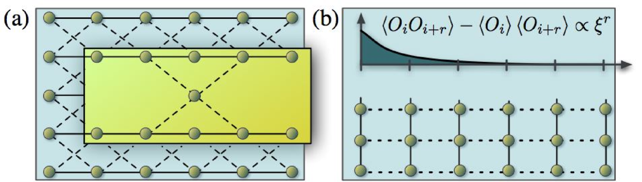
Figure 1: Two resources for universal measurement-based quantum computing. Fig. 1a depicts a weighted graph state, where solid lines correspond to a controlled $\pi$-phase gate, dashed lines to $\pi/2$. Fig. 1b represents a scheme deriving from an AKLT-type model. Dashed lines represent a state with non-vanishing correlation functions, solid lines correspond to $\pi$-phase gates in the $\{\mbox{$|1\rangle$},\mbox{$|2\rangle$}\}$-subspace.

To exemplify the power of our framework, we describe three new models for MBC in quantum mechanical lattice systems. In all these models, the randomness is compensated in a manner different from the $QC_{\cal C}$. They are chosen to highlight that, intriguingly, many properties of the original one-way computer may be relaxed, while still retaining a universal model for quantum computing: (i) We find resources exhibiting non-vanishing two-point correlations (which are typical for natural many-body ground states). The original discussion of the $QC_{\mathcal{C}}$ depended on the fact that the cluster can be prepared by mutually commuting unitaries (technically a quantum cellular automaton (QCA) [12]). Commutativity enables one to logically break down a $QC_{\cal C}$-calculation into small parts corresponding to individual gates; however, it implies severe restrictions, such as that the correlations vanish completely outside some neighborhood. Hence our framework can prove universality for states not amenable to any QCA-based technique. (ii) We treat a universal weighted graph state with partly weakly entangled bonds. (iii) In the final part – using different techniques – we present a family of states which are universal, yet are locally arbitrarily close to a pure state.

Matrix product states. – Starting point in the 1-D setting is the familiar notion of a matrix product state (MPS) [10]. We will first look at the simple case of a chain of $n$ qubits. Its state is specified by (i) an auxiliary $D$-dimensional Hilbert space, called correlation space, (ii) two operators $A[0],A[1]$ on $\mathbb{C}^{D}$, and (iii) two vectors $\mbox{$|L\rangle$},\mbox{$|R\rangle$}$ representing boundary conditions. One has explicitly

$$\mbox{$|\Psi\rangle$}=\sum_{s_{1},\dots,s_{n}=0,1}\mbox{$\langle R|$}A[s_{n}]\dots A[s_{1}]\mbox{$|L\rangle$}\,\,\mbox{$|s_{1},\dots,s_{n}\rangle$}.$$ (1)

In order to generalize Eq. (1) to 2-D lattices, we need to cast it into the form of a tensor network. Setting $L_{i}=\mbox{$\langle i|L\rangle$},A[s]_{i,j}=\mbox{$\langle j|$}A\mbox{$|i\rangle$},$ we arrive at $\langle s_{1},\dots,s_{n}|\Psi\rangle=\sum_{i_{0},\dots,i_{n}}^{D}L_{i_{0}}A[s_{1}]_{i_{0},i_{1}}\dots A[s_{n}]_{i_{n-1},i_{n}}{R^{\dagger}}_{i_{n}}$.

Computational tensor networks. – While the 1-D setting is awkward enough, the 2-D equivalent is completely unintelligible. To cure this problem, we introduce a graphical notation [15] which enables an intuitive understanding beyond the 1-D case. Tensors will be represented by boxes, indices by edges:

$$L_{r}=\lx@xy@svg{\hbox{\raise 0.0pt\hbox{\kern 6.40279pt\hbox{\ignorespaces\ignorespaces\ignorespaces\hbox{\vtop{\kern 0.0pt\offinterlineskip\halign{\entry@#!@&&\entry@@#!@\cr&\crcr}}}\ignorespaces{{{\hbox{\framed@@{0.0pt}}}}\hbox{\kern-6.40279pt\raise 0.0pt\hbox{\hbox{\kern 3.0pt\raise-3.41666pt\hbox{$\textstyle{L}$}}}}}\ignorespaces\ignorespaces\ignorespaces\ignorespaces{}{\hbox{\lx@xy@droprule}}\ignorespaces{}{\hbox{\lx@xy@droprule}}{\hbox{\lx@xy@droprule}}{\hbox{\kern 20.62915pt\raise 0.0pt\hbox{\hbox{\kern 0.0pt\raise 0.0pt\hbox{\hbox{\kern 3.0pt\raise 0.0pt\hbox{$\textstyle{}$}}}}}}}\ignorespaces}}}}\ignorespaces,\,A[s]_{l,r}=\lx@xy@svg{\hbox{\raise 0.0pt\hbox{\kern 3.0pt\hbox{\ignorespaces\ignorespaces\ignorespaces\hbox{\vtop{\kern 0.0pt\offinterlineskip\halign{\entry@#!@&&\entry@@#!@\cr&&\crcr}}}\ignorespaces{\hbox{\kern-3.0pt\raise 0.0pt\hbox{\hbox{\kern 0.0pt\raise 0.0pt\hbox{\hbox{\kern 3.0pt\raise 0.0pt\hbox{$\textstyle{\ignorespaces\ignorespaces\ignorespaces\ignorespaces}$}}}}}}}\ignorespaces\ignorespaces\ignorespaces\ignorespaces{}{\hbox{\lx@xy@droprule}}\ignorespaces{}{\hbox{\lx@xy@droprule}}{\hbox{\lx@xy@droprule}}{{{\hbox{\framed@@{0.0pt}}}}\hbox{\kern 17.22636pt\raise 0.0pt\hbox{\hbox{\kern 3.0pt\raise-2.5pt\hbox{$\textstyle{A[s]}$}}}}}\ignorespaces\ignorespaces\ignorespaces\ignorespaces{}{\hbox{\lx@xy@droprule}}\ignorespaces{}{\hbox{\lx@xy@droprule}}{\hbox{\lx@xy@droprule}}{\hbox{\kern 55.1958pt\raise 0.0pt\hbox{\hbox{\kern 0.0pt\raise 0.0pt\hbox{\hbox{\kern 3.0pt\raise 0.0pt\hbox{$\textstyle{}$}}}}}}}\ignorespaces}}}}\ignorespaces,\,{R^{\dagger}}_{l}=\lx@xy@svg{\hbox{\raise 0.0pt\hbox{\kern 3.0pt\hbox{\ignorespaces\ignorespaces\ignorespaces\hbox{\vtop{\kern 0.0pt\offinterlineskip\halign{\entry@#!@&&\entry@@#!@\cr&\crcr}}}\ignorespaces{\hbox{\kern-3.0pt\raise 0.0pt\hbox{\hbox{\kern 0.0pt\raise 0.0pt\hbox{\hbox{\kern 3.0pt\raise 0.0pt\hbox{$\textstyle{\ignorespaces\ignorespaces\ignorespaces\ignorespaces}$}}}}}}}\ignorespaces\ignorespaces\ignorespaces\ignorespaces{}{\hbox{\lx@xy@droprule}}\ignorespaces{}{\hbox{\lx@xy@droprule}}{\hbox{\lx@xy@droprule}}{{{\hbox{\framed@@{0.0pt}}}}\hbox{\kern 17.22636pt\raise 0.0pt\hbox{\hbox{\kern 3.0pt\raise-4.38889pt\hbox{$\textstyle{R^{\dagger}}$}}}}}\ignorespaces}}}}\ignorespaces. \textstyle{L} \textstyle{A[s]} \textstyle{R^{\dagger}} \textstyle{L} \textstyle{A[s]} \textstyle{R^{\dagger}}$$

A single-index tensor can be interpreted as the expansion coefficients of either a “ket” or a “bra”. Sometimes, we will indicate what interpretation we have in mind by placing arrows on the edges: outgoing arrows designating “kets”, incoming arrows “bras”. Connected arrows designate contractions of the respective indices. If $|\phi\rangle$ is a general state vector in $\mathbb{C}^{2}$, we abbreviate $\mbox{$\langle\phi|0\rangle$}\,A[0]+\mbox{$\langle\phi|1\rangle$}\,A[1]$ by $A[\phi]$. The overlap of $|\Psi\rangle$ with a local projection operator is easily derived:

$$\big{(}\bigotimes_{i}^{n}\mbox{$\langle\phi_{i}|$}\big{)}\mbox{$|\Psi\rangle$}=\lx@xy@svg{\hbox{\raise 0.0pt\hbox{\kern 6.40279pt\hbox{\ignorespaces\ignorespaces\ignorespaces\hbox{\vtop{\kern 0.0pt\offinterlineskip\halign{\entry@#!@&&\entry@@#!@\cr&&&&\crcr}}}\ignorespaces{{{\hbox{\framed@@{0.0pt}}}}\hbox{\kern-6.40279pt\raise 0.0pt\hbox{\hbox{\kern 3.0pt\raise-3.41666pt\hbox{$\textstyle{L}$}}}}}\ignorespaces\ignorespaces\ignorespaces\ignorespaces{}{\hbox{\lx@xy@droprule}}\ignorespaces{\hbox{\kern 9.24805pt\raise 0.0pt\hbox{\hbox{\kern 0.0pt\raise 0.0pt\hbox{\lx@xy@tip{1}\lx@xy@tip{-1}}}}}}{\hbox{\lx@xy@droprule}}{\hbox{\lx@xy@droprule}}{{{\hbox{\framed@@{0.0pt}}}}\hbox{\kern 9.24805pt\raise 0.0pt\hbox{\hbox{\kern 3.0pt\raise-2.5pt\hbox{$\textstyle{A[\phi_{1}]}$}}}}}\ignorespaces\ignorespaces\ignorespaces\ignorespaces{}{\hbox{\lx@xy@droprule}}\ignorespaces{\hbox{\kern 39.90724pt\raise 0.0pt\hbox{\hbox{\kern 0.0pt\raise 0.0pt\hbox{\lx@xy@tip{1}\lx@xy@tip{-1}}}}}}{\hbox{\lx@xy@droprule}}{\hbox{\lx@xy@droprule}}{\hbox{\kern 39.90724pt\raise 0.0pt\hbox{\hbox{\kern 0.0pt\raise 0.0pt\hbox{\hbox{\kern 3.0pt\raise 0.0pt\hbox{$\textstyle{\dots\ignorespaces\ignorespaces\ignorespaces\ignorespaces}$}}}}}}}\ignorespaces\ignorespaces\ignorespaces\ignorespaces{}{\hbox{\lx@xy@droprule}}\ignorespaces{\hbox{\kern 56.2525pt\raise 0.0pt\hbox{\hbox{\kern 0.0pt\raise 0.0pt\hbox{\lx@xy@tip{1}\lx@xy@tip{-1}}}}}}{\hbox{\lx@xy@droprule}}{\hbox{\lx@xy@droprule}}{{{\hbox{\framed@@{0.0pt}}}}\hbox{\kern 56.2525pt\raise 0.0pt\hbox{\hbox{\kern 3.0pt\raise-2.5pt\hbox{$\textstyle{A[\phi_{n}]}$}}}}}\ignorespaces\ignorespaces\ignorespaces\ignorespaces{}{\hbox{\lx@xy@droprule}}\ignorespaces{\hbox{\kern 87.473pt\raise 0.0pt\hbox{\hbox{\kern 0.0pt\raise 0.0pt\hbox{\lx@xy@tip{1}\lx@xy@tip{-1}}}}}}{\hbox{\lx@xy@droprule}}{\hbox{\lx@xy@droprule}}{{{\hbox{\framed@@{0.0pt}}}}\hbox{\kern 87.473pt\raise 0.0pt\hbox{\hbox{\kern 3.0pt\raise-4.38889pt\hbox{$\textstyle{R^{\dagger}}$}}}}}\ignorespaces}}}}\ignorespaces. \textstyle{L} \textstyle{A[\phi_{1}]} \textstyle{\dots\ignorespaces\ignorespaces\ignorespaces\ignorespaces} \textstyle{A[\phi_{n}]} \textstyle{R^{\dagger}} \textstyle{L} \textstyle{A[\phi_{1}]} \textstyle{\dots\ignorespaces\ignorespaces\ignorespaces\ignorespaces} \textstyle{A[\phi_{n}]} \textstyle{R^{\dagger}}$$ (2)

Eq. (2) should be read as follows: Initially, the correlation system is in the state $|L\rangle$. Subsequent measurements of local observables with eigenvectors $|\phi_{i}\rangle$ at the $i$-th site induce the evolution $A[\phi_{i}]$, thereby “processing” the state in the correlation space. The probability of a certain sequence of measurements to occur is given by the overlap of the resulting state vector with $|R\rangle$. An appealing perspective on MBC suggests itself: Measurement-based computing takes place in correlation space; the gates acting on the correlation systems are determined by local measurements. The crucial new insight compared to previous treatments of MPS and PEPS in the context of many-body physics [10, 11] or MBC [8] is that the matrices used in the parametrization of an MPS can be directly understood as quantum gates on a logical space. We will refer to this representation of MBC, as a computational tensor network (CTN).

The graphical notation greatly facilitates the passage to 2-D lattices. Here, the tensors $A[0/1]$ have four indices $A[s]_{l,d,r,u}$, which will be contracted with the indices of the left, right, upper and lower neighboring tensors respectively:

$$\mbox{$\langle s_{1,1},\dots,s_{2,2}|\Psi\rangle$}=\lx@xy@svg{\hbox{\raise 0.0pt\hbox{\kern 56.9402pt\hbox{{\hbox{\kern-56.9402pt\raise 0.0pt\hbox{\hbox{\kern 0.0pt\raise 31.34576pt\lx@xy@svgnested{\hbox{\raise 0.0pt\hbox{\kern 6.40279pt\hbox{\ignorespaces\ignorespaces\ignorespaces\hbox{\vtop{\kern 0.0pt\offinterlineskip\halign{\entry@#!@&&\entry@@#!@\cr&&\\&&&\\&&&\\&&\crcr}}}\ignorespaces{\hbox{\kern-3.0pt\raise 0.0pt\hbox{\hbox{\kern 0.0pt\raise 0.0pt\hbox{\hbox{\kern 3.0pt\raise 0.0pt\hbox{$\textstyle{}$}}}}}}}{{{\hbox{\framed@@{0.0pt}}}}\hbox{\kern 23.4289pt\raise 0.0pt\hbox{\hbox{\kern 3.0pt\raise-3.41666pt\hbox{$\textstyle{U}$}}}}}{{{\hbox{\framed@@{0.0pt}}}}\hbox{\kern 62.86333pt\raise 0.0pt\hbox{\hbox{\kern 3.0pt\raise-3.41666pt\hbox{$\textstyle{U}$}}}}}{{{\hbox{\framed@@{0.0pt}}}}\hbox{\kern-6.40279pt\raise-20.30385pt\hbox{\hbox{\kern 3.0pt\raise-3.41666pt\hbox{$\textstyle{L}$}}}}}\ignorespaces\ignorespaces\ignorespaces\ignorespaces{}{\hbox{\lx@xy@droprule}}\ignorespaces{\hbox{\kern 14.9386pt\raise-20.30385pt\hbox{\hbox{\kern 0.0pt\raise 0.0pt\hbox{\lx@xy@tip{1}\lx@xy@tip{-1}}}}}}{\hbox{\lx@xy@droprule}}{\hbox{\lx@xy@droprule}}{{{\hbox{\framed@@{0.0pt}}}}\hbox{\kern 14.9386pt\raise-20.30385pt\hbox{\hbox{\kern 3.0pt\raise-2.30334pt\hbox{$\textstyle{A[s_{1,1}]}$}}}}}\ignorespaces\ignorespaces\ignorespaces\ignorespaces{}{\hbox{\lx@xy@droprule}}\ignorespaces{\hbox{\kern 30.38791pt\raise-6.41666pt\hbox{\hbox{\kern 0.0pt\raise 0.0pt\hbox{\lx@xy@tip{1}\lx@xy@tip{-1}}}}}}{\hbox{\lx@xy@droprule}}{\hbox{\lx@xy@droprule}}\ignorespaces\ignorespaces\ignorespaces\ignorespaces{}{\hbox{\lx@xy@droprule}}\ignorespaces{\hbox{\kern 54.37303pt\raise-20.30385pt\hbox{\hbox{\kern 0.0pt\raise 0.0pt\hbox{\lx@xy@tip{1}\lx@xy@tip{-1}}}}}}{\hbox{\lx@xy@droprule}}{\hbox{\lx@xy@droprule}}{{{\hbox{\framed@@{0.0pt}}}}\hbox{\kern 54.37303pt\raise-20.30385pt\hbox{\hbox{\kern 3.0pt\raise-2.30334pt\hbox{$\textstyle{A[s_{2,1}]}$}}}}}\ignorespaces\ignorespaces\ignorespaces\ignorespaces{}{\hbox{\lx@xy@droprule}}\ignorespaces{\hbox{\kern 69.82234pt\raise-6.41666pt\hbox{\hbox{\kern 0.0pt\raise 0.0pt\hbox{\lx@xy@tip{1}\lx@xy@tip{-1}}}}}}{\hbox{\lx@xy@droprule}}{\hbox{\lx@xy@droprule}}\ignorespaces\ignorespaces\ignorespaces\ignorespaces{}{\hbox{\lx@xy@droprule}}\ignorespaces{\hbox{\kern 93.80746pt\raise-20.30385pt\hbox{\hbox{\kern 0.0pt\raise 0.0pt\hbox{\lx@xy@tip{1}\lx@xy@tip{-1}}}}}}{\hbox{\lx@xy@droprule}}{\hbox{\lx@xy@droprule}}{{{\hbox{\framed@@{0.0pt}}}}\hbox{\kern 93.80746pt\raise-20.30385pt\hbox{\hbox{\kern 3.0pt\raise-3.41666pt\hbox{$\textstyle{R}$}}}}}{{{\hbox{\framed@@{0.0pt}}}}\hbox{\kern-6.40279pt\raise-42.3877pt\hbox{\hbox{\kern 3.0pt\raise-3.41666pt\hbox{$\textstyle{L}$}}}}}\ignorespaces\ignorespaces\ignorespaces\ignorespaces{}{\hbox{\lx@xy@droprule}}\ignorespaces{\hbox{\kern 14.9386pt\raise-42.3877pt\hbox{\hbox{\kern 0.0pt\raise 0.0pt\hbox{\lx@xy@tip{1}\lx@xy@tip{-1}}}}}}{\hbox{\lx@xy@droprule}}{\hbox{\lx@xy@droprule}}{{{\hbox{\framed@@{0.0pt}}}}\hbox{\kern 14.9386pt\raise-42.3877pt\hbox{\hbox{\kern 3.0pt\raise-2.30334pt\hbox{$\textstyle{A[s_{1,2}]}$}}}}}\ignorespaces\ignorespaces\ignorespaces\ignorespaces{}{\hbox{\lx@xy@droprule}}\ignorespaces{\hbox{\kern 30.38791pt\raise-28.50052pt\hbox{\hbox{\kern 0.0pt\raise 0.0pt\hbox{\lx@xy@tip{1}\lx@xy@tip{-1}}}}}}{\hbox{\lx@xy@droprule}}{\hbox{\lx@xy@droprule}}\ignorespaces\ignorespaces\ignorespaces\ignorespaces{}{\hbox{\lx@xy@droprule}}\ignorespaces{\hbox{\kern 54.37303pt\raise-42.3877pt\hbox{\hbox{\kern 0.0pt\raise 0.0pt\hbox{\lx@xy@tip{1}\lx@xy@tip{-1}}}}}}{\hbox{\lx@xy@droprule}}{\hbox{\lx@xy@droprule}}{{{\hbox{\framed@@{0.0pt}}}}\hbox{\kern 54.37303pt\raise-42.3877pt\hbox{\hbox{\kern 3.0pt\raise-2.30334pt\hbox{$\textstyle{A[s_{2,2}]}$}}}}}\ignorespaces\ignorespaces\ignorespaces\ignorespaces{}{\hbox{\lx@xy@droprule}}\ignorespaces{\hbox{\kern 69.82234pt\raise-28.50052pt\hbox{\hbox{\kern 0.0pt\raise 0.0pt\hbox{\lx@xy@tip{1}\lx@xy@tip{-1}}}}}}{\hbox{\lx@xy@droprule}}{\hbox{\lx@xy@droprule}}\ignorespaces\ignorespaces\ignorespaces\ignorespaces{}{\hbox{\lx@xy@droprule}}\ignorespaces{\hbox{\kern 93.80746pt\raise-42.3877pt\hbox{\hbox{\kern 0.0pt\raise 0.0pt\hbox{\lx@xy@tip{1}\lx@xy@tip{-1}}}}}}{\hbox{\lx@xy@droprule}}{\hbox{\lx@xy@droprule}}{{{\hbox{\framed@@{0.0pt}}}}\hbox{\kern 93.80746pt\raise-42.3877pt\hbox{\hbox{\kern 3.0pt\raise-3.41666pt\hbox{$\textstyle{R}$}}}}}{\hbox{\kern-3.0pt\raise-62.69154pt\hbox{\hbox{\kern 0.0pt\raise 0.0pt\hbox{\hbox{\kern 3.0pt\raise 0.0pt\hbox{$\textstyle{}$}}}}}}}{{{\hbox{\framed@@{0.0pt}}}}\hbox{\kern 23.10944pt\raise-62.69154pt\hbox{\hbox{\kern 3.0pt\raise-3.41666pt\hbox{$\textstyle{D}$}}}}}\ignorespaces\ignorespaces\ignorespaces\ignorespaces{}{\hbox{\lx@xy@droprule}}\ignorespaces{\hbox{\kern 30.38791pt\raise-50.58437pt\hbox{\hbox{\kern 0.0pt\raise 0.0pt\hbox{\lx@xy@tip{1}\lx@xy@tip{-1}}}}}}{\hbox{\lx@xy@droprule}}{\hbox{\lx@xy@droprule}}{{{\hbox{\framed@@{0.0pt}}}}\hbox{\kern 62.54387pt\raise-62.69154pt\hbox{\hbox{\kern 3.0pt\raise-3.41666pt\hbox{$\textstyle{D}$}}}}}\ignorespaces\ignorespaces\ignorespaces\ignorespaces{}{\hbox{\lx@xy@droprule}}\ignorespaces{\hbox{\kern 69.82234pt\raise-50.58437pt\hbox{\hbox{\kern 0.0pt\raise 0.0pt\hbox{\lx@xy@tip{1}\lx@xy@tip{-1}}}}}}{\hbox{\lx@xy@droprule}}{\hbox{\lx@xy@droprule}}\ignorespaces\ignorespaces}}}}}}}}}}}} \textstyle{U} \textstyle{U} \textstyle{L} \textstyle{A[s_{1,1}]} \textstyle{A[s_{2,1}]} \textstyle{R} \textstyle{L} \textstyle{A[s_{1,2}]} \textstyle{A[s_{2,2}]} \textstyle{R} \textstyle{D} \textstyle{D} \textstyle{U} \textstyle{U} \textstyle{L} \textstyle{A[s_{1,1}]} \textstyle{A[s_{2,1}]} \textstyle{R} \textstyle{L} \textstyle{A[s_{1,2}]} \textstyle{A[s_{2,2}]} \textstyle{R} \textstyle{D} \textstyle{D}$$ (11)

for various boundary conditions $L,D,R,U$. Notably, it is known [11] that classical computers cannot efficiently perform the contraction appearing in Eq. (11). This fact is an incarnation of the power of quantum computers and no problem to our approach. We will now describe several examples, demonstrating the versatility of our framework and showing how – surprisingly – many reasonable assumptions about universal resources turn out to be unnecessary. In what follows, we use the standard notation $X,Y,Z$ for the Pauli operators, $H$ for the Hadamard gate and $S=\operatorname{diag}(1,i)$ for the $\pi/4$-gate. The controlled $\phi$-phase gate is $|0,0\rangle\langle 0,0|+|0,1\rangle\langle 0,1|+|1,0\rangle\langle 1,0|+e^{i\phi}|1,1\rangle\langle 1,1|$. Lastly, $\mbox{$|\pm\rangle$}=2^{-1/2}(\mbox{$|0\rangle$}\pm\mbox{$|1\rangle$})$.

Two-point correlations. – Here we consider a resource with exponentially decaying correlation functions, in a way as it occurs in ground states, but not in states resulting from a QCA. To be brief, we first describe a 1-D setting, turning to 2-D structures later. Define $G:=\exp(i\pi/kX)$ for some integer $k>2$. The relations

$$\lx@xy@svg{\hbox{\raise 0.0pt\hbox{\kern 3.0pt\hbox{\ignorespaces\ignorespaces\ignorespaces\hbox{\vtop{\kern 0.0pt\offinterlineskip\halign{\entry@#!@&&\entry@@#!@\cr&&\crcr}}}\ignorespaces{\hbox{\kern-3.0pt\raise 0.0pt\hbox{\hbox{\kern 0.0pt\raise 0.0pt\hbox{\hbox{\kern 3.0pt\raise 0.0pt\hbox{$\textstyle{\ignorespaces\ignorespaces\ignorespaces\ignorespaces}$}}}}}}}\ignorespaces\ignorespaces\ignorespaces\ignorespaces{}{\hbox{\lx@xy@droprule}}\ignorespaces{\hbox{\kern 14.38109pt\raise 0.0pt\hbox{\hbox{\kern 0.0pt\raise 0.0pt\hbox{\lx@xy@tip{1}\lx@xy@tip{-1}}}}}}{\hbox{\lx@xy@droprule}}{\hbox{\lx@xy@droprule}}{{{\hbox{\framed@@{0.0pt}}}}\hbox{\kern 14.38109pt\raise 0.0pt\hbox{\hbox{\kern 3.0pt\raise-2.5pt\hbox{$\textstyle{A[s]}$}}}}}\ignorespaces\ignorespaces\ignorespaces\ignorespaces{}{\hbox{\lx@xy@droprule}}\ignorespaces{\hbox{\kern 49.50525pt\raise 0.0pt\hbox{\hbox{\kern 0.0pt\raise 0.0pt\hbox{\lx@xy@tip{1}\lx@xy@tip{-1}}}}}}{\hbox{\lx@xy@droprule}}{\hbox{\lx@xy@droprule}}{\hbox{\kern 49.50525pt\raise 0.0pt\hbox{\hbox{\kern 0.0pt\raise 0.0pt\hbox{\hbox{\kern 3.0pt\raise 0.0pt\hbox{$\textstyle{}$}}}}}}}\ignorespaces}}}}\ignorespaces=G\mbox{$|s\rangle$}_{r}\mbox{$\langle s|$}_{l},\quad\mbox{$|L\rangle$}=\mbox{$|+\rangle$},\quad\mbox{$|R\rangle$}=G^{-1}\mbox{$|+\rangle$} \textstyle{A[s]} \textstyle{A[s]}$$

define a state vector $|\Psi\rangle$ for a chain of qubits. The two-point correlations never vanish completely: One finds [10] that

$$\langle Z_{i}Z_{i+n+1}\rangle-\langle Z_{i}\rangle\,\langle Z_{i+n+1}\rangle\propto\xi^{n},$$

where $\xi=2\sin^{2}(\pi/k)-1$. Still, all single-qubit unitaries on the correlation system can be realized by local physical measurements. Ignoring global factors (as we will do when possible), one computes:

$$\lx@xy@svg{\hbox{\raise 0.0pt\hbox{\kern 3.0pt\hbox{\ignorespaces\ignorespaces\ignorespaces\hbox{\vtop{\kern 0.0pt\offinterlineskip\halign{\entry@#!@&&\entry@@#!@\cr&&\crcr}}}\ignorespaces{\hbox{\kern-3.0pt\raise 0.0pt\hbox{\hbox{\kern 0.0pt\raise 0.0pt\hbox{\hbox{\kern 3.0pt\raise 0.0pt\hbox{$\textstyle{\ignorespaces\ignorespaces\ignorespaces\ignorespaces}$}}}}}}}\ignorespaces\ignorespaces\ignorespaces\ignorespaces{}{\hbox{\lx@xy@droprule}}\ignorespaces{\hbox{\kern 11.53581pt\raise 0.0pt\hbox{\hbox{\kern 0.0pt\raise 0.0pt\hbox{\lx@xy@tip{1}\lx@xy@tip{-1}}}}}}{\hbox{\lx@xy@droprule}}{\hbox{\lx@xy@droprule}}{{{\hbox{\framed@@{0.0pt}}}}\hbox{\kern 11.53581pt\raise 0.0pt\hbox{\hbox{\kern 3.0pt\raise-2.5pt\hbox{$\textstyle{A[+]}$}}}}}\ignorespaces\ignorespaces\ignorespaces\ignorespaces{}{\hbox{\lx@xy@droprule}}\ignorespaces{\hbox{\kern 46.905pt\raise 0.0pt\hbox{\hbox{\kern 0.0pt\raise 0.0pt\hbox{\lx@xy@tip{1}\lx@xy@tip{-1}}}}}}{\hbox{\lx@xy@droprule}}{\hbox{\lx@xy@droprule}}{\hbox{\kern 46.905pt\raise 0.0pt\hbox{\hbox{\kern 0.0pt\raise 0.0pt\hbox{\hbox{\kern 3.0pt\raise 0.0pt\hbox{$\textstyle{}$}}}}}}}\ignorespaces}}}}\ignorespaces=G,\lx@xy@svg{\hbox{\raise 0.0pt\hbox{\kern 3.0pt\hbox{\ignorespaces\ignorespaces\ignorespaces\hbox{\vtop{\kern 0.0pt\offinterlineskip\halign{\entry@#!@&&\entry@@#!@\cr&&\crcr}}}\ignorespaces{\hbox{\kern-3.0pt\raise 0.0pt\hbox{\hbox{\kern 0.0pt\raise 0.0pt\hbox{\hbox{\kern 3.0pt\raise 0.0pt\hbox{$\textstyle{\ignorespaces\ignorespaces\ignorespaces\ignorespaces}$}}}}}}}\ignorespaces\ignorespaces\ignorespaces\ignorespaces{}{\hbox{\lx@xy@droprule}}\ignorespaces{\hbox{\kern 14.38109pt\raise 0.0pt\hbox{\hbox{\kern 0.0pt\raise 0.0pt\hbox{\lx@xy@tip{1}\lx@xy@tip{-1}}}}}}{\hbox{\lx@xy@droprule}}{\hbox{\lx@xy@droprule}}{{{\hbox{\framed@@{0.0pt}}}}\hbox{\kern 14.38109pt\raise 0.0pt\hbox{\hbox{\kern 3.0pt\raise-2.5pt\hbox{$\textstyle{A[-]}$}}}}}\ignorespaces\ignorespaces\ignorespaces\ignorespaces{}{\hbox{\lx@xy@droprule}}\ignorespaces{\hbox{\kern 48.1511pt\raise 0.0pt\hbox{\hbox{\kern 0.0pt\raise 0.0pt\hbox{\lx@xy@tip{1}\lx@xy@tip{-1}}}}}}{\hbox{\lx@xy@droprule}}{\hbox{\lx@xy@droprule}}{\hbox{\kern 48.1511pt\raise 0.0pt\hbox{\hbox{\kern 0.0pt\raise 0.0pt\hbox{\hbox{\kern 3.0pt\raise 0.0pt\hbox{$\textstyle{}$}}}}}}}\ignorespaces}}}}\ignorespaces=GZ;\>\lx@xy@svg{\hbox{\raise 0.0pt\hbox{\kern 3.0pt\hbox{\ignorespaces\ignorespaces\ignorespaces\hbox{\vtop{\kern 0.0pt\offinterlineskip\halign{\entry@#!@&&\entry@@#!@\cr&&\crcr}}}\ignorespaces{\hbox{\kern-3.0pt\raise 0.0pt\hbox{\hbox{\kern 0.0pt\raise 0.0pt\hbox{\hbox{\kern 3.0pt\raise 0.0pt\hbox{$\textstyle{\ignorespaces\ignorespaces\ignorespaces\ignorespaces}$}}}}}}}\ignorespaces\ignorespaces\ignorespaces\ignorespaces{}{\hbox{\lx@xy@droprule}}\ignorespaces{\hbox{\kern 14.38109pt\raise 0.0pt\hbox{\hbox{\kern 0.0pt\raise 0.0pt\hbox{\lx@xy@tip{1}\lx@xy@tip{-1}}}}}}{\hbox{\lx@xy@droprule}}{\hbox{\lx@xy@droprule}}{{{\hbox{\framed@@{0.0pt}}}}\hbox{\kern 14.38109pt\raise 0.0pt\hbox{\hbox{\kern 3.0pt\raise-2.5pt\hbox{$\textstyle{A[X]}$}}}}}\ignorespaces\ignorespaces\ignorespaces\ignorespaces{}{\hbox{\lx@xy@droprule}}\ignorespaces{\hbox{\kern 53.88718pt\raise 0.0pt\hbox{\hbox{\kern 0.0pt\raise 0.0pt\hbox{\lx@xy@tip{1}\lx@xy@tip{-1}}}}}}{\hbox{\lx@xy@droprule}}{\hbox{\lx@xy@droprule}}{\hbox{\kern 53.88718pt\raise 0.0pt\hbox{\hbox{\kern 0.0pt\raise 0.0pt\hbox{\hbox{\kern 3.0pt\raise 0.0pt\hbox{$\textstyle{}$}}}}}}}\ignorespaces}}}}\ignorespaces\!\!\!\!\!=GZ^{x}, \textstyle{A[+]} \textstyle{A[-]} \textstyle{A[X]} \textstyle{A[+]} \textstyle{A[-]} \textstyle{A[X]}$$

where the r.h.s. is a compact notation for the two equations on the left: An observable as the argument to $A[\,]$ denotes a measurement in the corresponding eigenbasis. The outcome of the measurement is assigned to a variable; here $x=0$ in case of the $+1$-eigenvalue and $x=1$ in case of $-1$. Local $X$-basis measurements hence cause the state of the correlation system to be transported from left to right (up to local unitaries). When measuring several consecutive sites in the $X$-basis, the overall operator applied to the correlation system is given by $B:=\dots GZ^{x_{2}}GZ^{x_{1}}$. Assuming that we intended to just transport the information faithfully, we conceive $B$ as an unwanted by-product. To understand this structure, consider the following elementary statement: Let $A,B$ be matrices having finite order [18]. Every element in the group generated by $A,B$ can be written as $AB^{k_{1}}AB^{k_{2}}A\dots AB^{k_{n}}$ for some $n\in\mathbb{N}$ and $k_{i}\in\{0,1\}$. Applied to our situation: The by-product operators form a finite group $\mathcal{B}$ generated by $G,Z$. The group property gives a possibility to cope with by-products [19]: Assume that at some point the state vector of the correlation system is given by $B\mbox{$|\psi\rangle$}$, for some unwanted $B\in\mathcal{B}$. Transferring the state along the chain will introduce any by-product $B^{\prime}\in\mathcal{B}$ after a finite expected number of steps. In particular, $B^{\prime}=B^{-1}$ will occur, leaving us with $B^{-1}B\mbox{$|\psi\rangle$}=\mbox{$|\psi\rangle$}$. Note that this technique is completely general: it can deal with any finite by-product group (see further examples below). Moving on, a measurement in the $2^{-1/2}(\mbox{$|0\rangle$}\pm e^{i\phi}\mbox{$|1\rangle$}$ basis induces the operator $S(\phi):=\operatorname{diag}(1,e^{i\phi})$ on the correlation system (up to by-products). But by the preceding discussion, we can also implement $GS(\phi)G^{-1}$, which is sufficient to generate any single-qubit unitary [1]. Lastly, it is easy to see that $Z$-measurements prepare a known state in the correlation system and conversely can be used to read it out.

AKLT-type states. – In this example, we consider ground states of nearest-neighbor spin-1 Hamiltonians of the AKLT-type, as they are well-known in the context of condensed-matter physics [10]. We investigate ground-states induced by $\lx@xy@svg{\hbox{\raise 0.0pt\hbox{\kern 3.0pt\hbox{\ignorespaces\ignorespaces\ignorespaces\hbox{\vtop{\kern 0.0pt\offinterlineskip\halign{\entry@#!@&&\entry@@#!@\cr&&\crcr}}}\ignorespaces{\hbox{\kern-3.0pt\raise 0.0pt\hbox{\hbox{\kern 0.0pt\raise 0.0pt\hbox{\hbox{\kern 3.0pt\raise 0.0pt\hbox{$\textstyle{\ignorespaces\ignorespaces\ignorespaces\ignorespaces}$}}}}}}}\ignorespaces\ignorespaces\ignorespaces\ignorespaces{}{\hbox{\lx@xy@droprule}}\ignorespaces{\hbox{\kern 14.38109pt\raise 0.0pt\hbox{\hbox{\kern 0.0pt\raise 0.0pt\hbox{\lx@xy@tip{1}\lx@xy@tip{-1}}}}}}{\hbox{\lx@xy@droprule}}{\hbox{\lx@xy@droprule}}{{{\hbox{\framed@@{0.0pt}}}}\hbox{\kern 14.38109pt\raise 0.0pt\hbox{\hbox{\kern 3.0pt\raise-2.5pt\hbox{$\textstyle{A[0]}$}}}}}\ignorespaces\ignorespaces\ignorespaces\ignorespaces{}{\hbox{\lx@xy@droprule}}\ignorespaces{\hbox{\kern 49.81778pt\raise 0.0pt\hbox{\hbox{\kern 0.0pt\raise 0.0pt\hbox{\lx@xy@tip{1}\lx@xy@tip{-1}}}}}}{\hbox{\lx@xy@droprule}}{\hbox{\lx@xy@droprule}}{\hbox{\kern 49.81778pt\raise 0.0pt\hbox{\hbox{\kern 0.0pt\raise 0.0pt\hbox{\hbox{\kern 3.0pt\raise 0.0pt\hbox{$\textstyle{}$}}}}}}}\ignorespaces}}}}\ignorespaces=H$, $\lx@xy@svg{\hbox{\raise 0.0pt\hbox{\kern 3.0pt\hbox{\ignorespaces\ignorespaces\ignorespaces\hbox{\vtop{\kern 0.0pt\offinterlineskip\halign{\entry@#!@&&\entry@@#!@\cr&&\crcr}}}\ignorespaces{\hbox{\kern-3.0pt\raise 0.0pt\hbox{\hbox{\kern 0.0pt\raise 0.0pt\hbox{\hbox{\kern 3.0pt\raise 0.0pt\hbox{$\textstyle{\ignorespaces\ignorespaces\ignorespaces\ignorespaces}$}}}}}}}\ignorespaces\ignorespaces\ignorespaces\ignorespaces{}{\hbox{\lx@xy@droprule}}\ignorespaces{\hbox{\kern 14.38109pt\raise 0.0pt\hbox{\hbox{\kern 0.0pt\raise 0.0pt\hbox{\lx@xy@tip{1}\lx@xy@tip{-1}}}}}}{\hbox{\lx@xy@droprule}}{\hbox{\lx@xy@droprule}}{{{\hbox{\framed@@{0.0pt}}}}\hbox{\kern 14.38109pt\raise 0.0pt\hbox{\hbox{\kern 3.0pt\raise-2.5pt\hbox{$\textstyle{A[1]}$}}}}}\ignorespaces\ignorespaces\ignorespaces\ignorespaces{}{\hbox{\lx@xy@droprule}}\ignorespaces{\hbox{\kern 49.81778pt\raise 0.0pt\hbox{\hbox{\kern 0.0pt\raise 0.0pt\hbox{\lx@xy@tip{1}\lx@xy@tip{-1}}}}}}{\hbox{\lx@xy@droprule}}{\hbox{\lx@xy@droprule}}{\hbox{\kern 49.81778pt\raise 0.0pt\hbox{\hbox{\kern 0.0pt\raise 0.0pt\hbox{\hbox{\kern 3.0pt\raise 0.0pt\hbox{$\textstyle{}$}}}}}}}\ignorespaces}}}}\ignorespaces=(X-iY)2^{-1/2}$, $\lx@xy@svg{\hbox{\raise 0.0pt\hbox{\kern 3.0pt\hbox{\ignorespaces\ignorespaces\ignorespaces\hbox{\vtop{\kern 0.0pt\offinterlineskip\halign{\entry@#!@&&\entry@@#!@\cr&&\crcr}}}\ignorespaces{\hbox{\kern-3.0pt\raise 0.0pt\hbox{\hbox{\kern 0.0pt\raise 0.0pt\hbox{\hbox{\kern 3.0pt\raise 0.0pt\hbox{$\textstyle{\ignorespaces\ignorespaces\ignorespaces\ignorespaces}$}}}}}}}\ignorespaces\ignorespaces\ignorespaces\ignorespaces{}{\hbox{\lx@xy@droprule}}\ignorespaces{\hbox{\kern 14.38109pt\raise 0.0pt\hbox{\hbox{\kern 0.0pt\raise 0.0pt\hbox{\lx@xy@tip{1}\lx@xy@tip{-1}}}}}}{\hbox{\lx@xy@droprule}}{\hbox{\lx@xy@droprule}}{{{\hbox{\framed@@{0.0pt}}}}\hbox{\kern 14.38109pt\raise 0.0pt\hbox{\hbox{\kern 3.0pt\raise-2.5pt\hbox{$\textstyle{A[2]}$}}}}}\ignorespaces\ignorespaces\ignorespaces\ignorespaces{}{\hbox{\lx@xy@droprule}}\ignorespaces{\hbox{\kern 49.81778pt\raise 0.0pt\hbox{\hbox{\kern 0.0pt\raise 0.0pt\hbox{\lx@xy@tip{1}\lx@xy@tip{-1}}}}}}{\hbox{\lx@xy@droprule}}{\hbox{\lx@xy@droprule}}{\hbox{\kern 49.81778pt\raise 0.0pt\hbox{\hbox{\kern 0.0pt\raise 0.0pt\hbox{\hbox{\kern 3.0pt\raise 0.0pt\hbox{$\textstyle{}$}}}}}}}\ignorespaces}}}}\ignorespaces=(X+iY)2^{-1/2}$. This is the exact unique ground state of a nearest-neighbor frustration-free gapped Hamiltonian (in the original AKLT model $H$ is replaced by $Z$ in the definition of $A[0]$). Proving that any single-qubit unitary can be realized on the correlation space commences in a similar way as before. Measurements in the $\{\mbox{$|0\rangle$},2^{-1/2}(\mbox{$|1\rangle$}\pm e^{i\phi}\mbox{$|2\rangle$})\}$-basis gives rise to $H,S(\phi)$ or $ZS(\phi)$, depending on the measurement outcome. The finite by-product group is in this case generated by $H,Z$. But that is all we need to show, as gates of the form $S(\phi),HS(\phi)H$ generate all of $SU(2)$.

Weighted graph states. – Both previous examples can be embedded into 2-D lattices, universal for computation (see Fig. 1b). A general technique for coupling 1-D chains to 2-D universal resources will be discussed by means of a further example: the weighted graph state [17, 4] shown in Fig. 1 (a). In the figure, vertices denote physical systems initially in $|+\rangle$, solid edges the application of a controlled $\pi$-phase gate and dashed edges controlled $\pi/2$-phases, so some of the entangling gates do not have maximal entangling power. The resource’s tensor representation (acting on a $D=2$-dimensional correlation space) is given by

$$\lx@xy@svg{\hbox{\raise 0.0pt\hbox{\kern 26.40735pt\hbox{{\hbox{\kern-26.40735pt\raise 0.0pt\hbox{\hbox{\kern 0.0pt\raise 13.84526pt\lx@xy@svgnested{\hbox{\raise 0.0pt\hbox{\kern 3.0pt\hbox{\ignorespaces\ignorespaces\ignorespaces\hbox{\vtop{\kern 0.0pt\offinterlineskip\halign{\entry@#!@&&\entry@@#!@\cr&&\\&&\\&&\crcr}}}\ignorespaces{\hbox{\kern-3.0pt\raise 0.0pt\hbox{\hbox{\kern 0.0pt\raise 0.0pt\hbox{\hbox{\kern 3.0pt\raise 0.0pt\hbox{$\textstyle{}$}}}}}}}{\hbox{\kern 20.40735pt\raise 0.0pt\hbox{\hbox{\kern 0.0pt\raise 0.0pt\hbox{\hbox{\kern 3.0pt\raise 0.0pt\hbox{$\textstyle{}$}}}}}}}{\hbox{\kern 43.8147pt\raise 0.0pt\hbox{\hbox{\kern 0.0pt\raise 0.0pt\hbox{\hbox{\kern 3.0pt\raise 0.0pt\hbox{$\textstyle{}$}}}}}}}{\hbox{\kern-3.0pt\raise-13.84526pt\hbox{\hbox{\kern 0.0pt\raise 0.0pt\hbox{\hbox{\kern 3.0pt\raise 0.0pt\hbox{$\textstyle{\ignorespaces\ignorespaces\ignorespaces\ignorespaces}$}}}}}}}\ignorespaces\ignorespaces\ignorespaces\ignorespaces{}{\hbox{\lx@xy@droprule}}\ignorespaces{\hbox{\kern 11.53581pt\raise-13.84526pt\hbox{\hbox{\kern 0.0pt\raise 0.0pt\hbox{\lx@xy@tip{1}\lx@xy@tip{-1}}}}}}{\hbox{\lx@xy@droprule}}{\hbox{\lx@xy@droprule}}{{{\hbox{\framed@@{0.0pt}}}}\hbox{\kern 11.53581pt\raise-13.84526pt\hbox{\hbox{\kern 3.0pt\raise-2.5pt\hbox{$\textstyle{A[s]}$}}}}}\ignorespaces\ignorespaces\ignorespaces{}\ignorespaces\ignorespaces{\hbox{\lx@xy@drawline@}}\ignorespaces{\hbox{\kern 3.0pt\raise-1.77246pt\hbox{\hbox{\kern 0.0pt\raise 0.0pt\hbox{\lx@xy@tip{1}\lx@xy@tip{-1}}}}}}\ignorespaces\ignorespaces{\hbox{\lx@xy@drawline@}}\ignorespaces{\hbox{\lx@xy@drawline@}}\ignorespaces\ignorespaces\ignorespaces\ignorespaces{}{\hbox{\lx@xy@droprule}}\ignorespaces{\hbox{\kern 43.8147pt\raise-13.84526pt\hbox{\hbox{\kern 0.0pt\raise 0.0pt\hbox{\lx@xy@tip{1}\lx@xy@tip{-1}}}}}}{\hbox{\lx@xy@droprule}}{\hbox{\lx@xy@droprule}}\ignorespaces\ignorespaces\ignorespaces{}\ignorespaces\ignorespaces{\hbox{\lx@xy@drawline@}}\ignorespaces{\hbox{\kern 43.8147pt\raise-1.77539pt\hbox{\hbox{\kern 0.0pt\raise 0.0pt\hbox{\lx@xy@tip{1}\lx@xy@tip{-1}}}}}}\ignorespaces\ignorespaces{\hbox{\lx@xy@drawline@}}\ignorespaces{\hbox{\lx@xy@drawline@}}{\hbox{\kern 43.8147pt\raise-13.84526pt\hbox{\hbox{\kern 0.0pt\raise 0.0pt\hbox{\hbox{\kern 3.0pt\raise 0.0pt\hbox{$\textstyle{}$}}}}}}}{\hbox{\kern-3.0pt\raise-27.69052pt\hbox{\hbox{\kern 0.0pt\raise 0.0pt\hbox{\hbox{\kern 3.0pt\raise 0.0pt\hbox{$\textstyle{\ignorespaces\ignorespaces\ignorespaces\ignorespaces}$}}}}}}}\ignorespaces\ignorespaces\ignorespaces{}\ignorespaces\ignorespaces{\hbox{\lx@xy@drawline@}}\ignorespaces{\hbox{\kern 11.53581pt\raise-20.87079pt\hbox{\hbox{\kern 0.0pt\raise 0.0pt\hbox{\lx@xy@tip{1}\lx@xy@tip{-1}}}}}}\ignorespaces\ignorespaces{\hbox{\lx@xy@drawline@}}\ignorespaces{\hbox{\lx@xy@drawline@}}{\hbox{\kern 20.40735pt\raise-27.69052pt\hbox{\hbox{\kern 0.0pt\raise 0.0pt\hbox{\hbox{\kern 3.0pt\raise 0.0pt\hbox{$\textstyle{}$}}}}}}}{\hbox{\kern 43.8147pt\raise-27.69052pt\hbox{\hbox{\kern 0.0pt\raise 0.0pt\hbox{\hbox{\kern 3.0pt\raise 0.0pt\hbox{$\textstyle{\ignorespaces\ignorespaces\ignorespaces\ignorespaces}$}}}}}}}\ignorespaces\ignorespaces\ignorespaces{}\ignorespaces\ignorespaces{\hbox{\lx@xy@drawline@}}\ignorespaces{\hbox{\kern 35.2789pt\raise-20.8592pt\hbox{\hbox{\kern 0.0pt\raise 0.0pt\hbox{\lx@xy@tip{1}\lx@xy@tip{-1}}}}}}\ignorespaces\ignorespaces{\hbox{\lx@xy@drawline@}}\ignorespaces{\hbox{\lx@xy@drawline@}}\ignorespaces\ignorespaces}}}}}}}}}}}}=S^{s}\mbox{$|+\rangle$}_{ru}\,S^{s}\mbox{$|+\rangle$}_{lu}\,Z^{s}\mbox{$|+\rangle$}_{r}\mbox{$\langle s|$}_{ld}\mbox{$\langle s|$}_{rd}\mbox{$\langle s|$}_{l}, \textstyle{A[s]} \textstyle{A[s]}$$ (13)

where $s\in\{0,1\}$. Indices are labeled $ru$ for “right-up” to $ld$ for “left-down”. Boundary conditions are $|0\rangle$ for the $ru,lu,r$-directions; $|+\rangle$ otherwise. The broad setting for our scheme is the following: the correlation system of every second horizontal line in the lattice is interpreted as a logical qubit. Intermediate lines will either be measured in the $Z$-eigenbasis – causing the logical bits to be isolated – or in the $Y$-basis – mediating an interaction between adjacent logical qubits.

We will first describe how to realize isolated evolutions of logical qubits. According to Eq. (13) the tensors $A[0/1]$ factor, allowing us to draw only the arrows corresponding to the factors of interest; so e.g. $\lx@xy@svg{\hbox{\raise 0.0pt\hbox{\kern 11.87154pt\hbox{\ignorespaces\ignorespaces\ignorespaces\hbox{\vtop{\kern 0.0pt\offinterlineskip\halign{\entry@#!@&&\entry@@#!@\cr&\crcr}}}\ignorespaces{{{\hbox{\framed@@{0.0pt}}}}\hbox{\kern-11.87154pt\raise 0.0pt\hbox{\hbox{\kern 3.0pt\raise-2.5pt\hbox{$\textstyle{A[s]}$}}}}}\ignorespaces\ignorespaces\ignorespaces\ignorespaces{}{\hbox{\lx@xy@droprule}}\ignorespaces{\hbox{\kern 23.25262pt\raise 0.0pt\hbox{\hbox{\kern 0.0pt\raise 0.0pt\hbox{\lx@xy@tip{1}\lx@xy@tip{-1}}}}}}{\hbox{\lx@xy@droprule}}{\hbox{\lx@xy@droprule}}{\hbox{\kern 23.25262pt\raise 0.0pt\hbox{\hbox{\kern 0.0pt\raise 0.0pt\hbox{\hbox{\kern 3.0pt\raise 0.0pt\hbox{$\textstyle{}$}}}}}}}\ignorespaces}}}}\ignorespaces=Z^{s}\mbox{$|+\rangle$}_{r}$. We find

$$\lx@xy@svg{\hbox{\raise 0.0pt\hbox{\kern 62.76192pt\hbox{{\hbox{\kern-62.76192pt\raise 0.0pt\hbox{\hbox{\kern 0.0pt\raise 16.26666pt\lx@xy@svgnested{\hbox{\raise 0.0pt\hbox{\kern 18.97725pt\hbox{\ignorespaces\ignorespaces\ignorespaces\hbox{\vtop{\kern 0.0pt\offinterlineskip\halign{\entry@#!@&&\entry@@#!@\cr&&\\&&\\&&\\}}}\ignorespaces{{{\hbox{\framed@@{0.0pt}}}}\hbox{\kern-18.97725pt\raise 0.0pt\hbox{\hbox{\kern 3.0pt\raise-2.28223pt\hbox{$\textstyle{A[Z_{i-1,u}]}$}}}}}{\hbox{\kern 39.5402pt\raise 0.0pt\hbox{\hbox{\kern 0.0pt\raise 0.0pt\hbox{\hbox{\kern 3.0pt\raise 0.0pt\hbox{$\textstyle{}$}}}}}}}{{{\hbox{\framed@@{0.0pt}}}}\hbox{\kern 66.10316pt\raise 0.0pt\hbox{\hbox{\kern 3.0pt\raise-2.28223pt\hbox{$\textstyle{A[Z_{i+1,u}]}$}}}}}{\hbox{\kern-3.0pt\raise-16.21777pt\hbox{\hbox{\kern 0.0pt\raise 0.0pt\hbox{\hbox{\kern 3.0pt\raise 0.0pt\hbox{$\textstyle{\ignorespaces\ignorespaces\ignorespaces\ignorespaces}$}}}}}}}\ignorespaces\ignorespaces\ignorespaces\ignorespaces{}{\hbox{\lx@xy@droprule}}\ignorespaces{\hbox{\kern 27.51306pt\raise-16.21777pt\hbox{\hbox{\kern 0.0pt\raise 0.0pt\hbox{\lx@xy@tip{1}\lx@xy@tip{-1}}}}}}{\hbox{\lx@xy@droprule}}{\hbox{\lx@xy@droprule}}{{{\hbox{\framed@@{0.0pt}}}}\hbox{\kern 27.51306pt\raise-16.21777pt\hbox{\hbox{\kern 3.0pt\raise-2.5pt\hbox{$\textstyle{A[X_{i}]}$}}}}}\ignorespaces\ignorespaces\ignorespaces{}\ignorespaces\ignorespaces{\hbox{\lx@xy@drawline@}}\ignorespaces{\hbox{\kern 18.97726pt\raise-7.20912pt\hbox{\hbox{\kern 0.0pt\raise 0.0pt\hbox{\lx@xy@tip{1}\lx@xy@tip{-1}}}}}}\ignorespaces\ignorespaces{\hbox{\lx@xy@drawline@}}\ignorespaces{\hbox{\lx@xy@drawline@}}\ignorespaces\ignorespaces\ignorespaces{}\ignorespaces\ignorespaces{\hbox{\lx@xy@drawline@}}\ignorespaces{\hbox{\kern 66.10316pt\raise-7.48439pt\hbox{\hbox{\kern 0.0pt\raise 0.0pt\hbox{\lx@xy@tip{1}\lx@xy@tip{-1}}}}}}\ignorespaces\ignorespaces{\hbox{\lx@xy@drawline@}}\ignorespaces{\hbox{\lx@xy@drawline@}}\ignorespaces\ignorespaces\ignorespaces\ignorespaces{}{\hbox{\lx@xy@droprule}}\ignorespaces{\hbox{\kern 83.32487pt\raise-16.21777pt\hbox{\hbox{\kern 0.0pt\raise 0.0pt\hbox{\lx@xy@tip{1}\lx@xy@tip{-1}}}}}}{\hbox{\lx@xy@droprule}}{\hbox{\lx@xy@droprule}}{\hbox{\kern 83.32487pt\raise-16.21777pt\hbox{\hbox{\kern 0.0pt\raise 0.0pt\hbox{\hbox{\kern 3.0pt\raise 0.0pt\hbox{$\textstyle{}$}}}}}}}{{{\hbox{\framed@@{0.0pt}}}}\hbox{\kern-18.83173pt\raise-32.48444pt\hbox{\hbox{\kern 3.0pt\raise-2.23334pt\hbox{$\textstyle{A[Z_{i-1,d}]}$}}}}}\ignorespaces\ignorespaces\ignorespaces{}\ignorespaces\ignorespaces{\hbox{\lx@xy@drawline@}}\ignorespaces{\hbox{\kern 27.51306pt\raise-21.97035pt\hbox{\hbox{\kern 0.0pt\raise 0.0pt\hbox{\lx@xy@tip{1}\lx@xy@tip{-1}}}}}}\ignorespaces\ignorespaces{\hbox{\lx@xy@drawline@}}\ignorespaces{\hbox{\lx@xy@drawline@}}{\hbox{\kern 39.5402pt\raise-32.48444pt\hbox{\hbox{\kern 0.0pt\raise 0.0pt\hbox{\hbox{\kern 3.0pt\raise 0.0pt\hbox{$\textstyle{}$}}}}}}}{{{\hbox{\framed@@{0.0pt}}}}\hbox{\kern 66.24869pt\raise-32.48444pt\hbox{\hbox{\kern 3.0pt\raise-2.23334pt\hbox{$\textstyle{A[Z_{i+1,d}]}$}}}}}\ignorespaces\ignorespaces\ignorespaces{}\ignorespaces\ignorespaces{\hbox{\lx@xy@drawline@}}\ignorespaces{\hbox{\kern 57.56735pt\raise-21.77957pt\hbox{\hbox{\kern 0.0pt\raise 0.0pt\hbox{\lx@xy@tip{1}\lx@xy@tip{-1}}}}}}\ignorespaces\ignorespaces{\hbox{\lx@xy@drawline@}}\ignorespaces{\hbox{\lx@xy@drawline@}}\ignorespaces\ignorespaces}}}}}}}}}}}}=HS^{2x_{i}+z_{i}}, \textstyle{A[Z_{i-1,u}]} \textstyle{A[Z_{i+1,u}]} \textstyle{A[X_{i}]} \textstyle{A[Z_{i-1,d}]} \textstyle{A[Z_{i+1,d}]} \textstyle{A[Z_{i-1,u}]} \textstyle{A[Z_{i+1,u}]} \textstyle{A[X_{i}]} \textstyle{A[Z_{i-1,d}]} \textstyle{A[Z_{i+1,d}]}$$ (14)

where $z_{i}=z_{i-1,u}+z_{i-1,d}+z_{i+1,u}+z_{i+1,d}$. Eq. (14) is of the kind treated before in the case of 1-D chains. Indeed, using the same techniques, one sees easily that general local unitaries can be implemented by measurements in the $2^{-1/2}(\mbox{$|0\rangle$}\pm e^{i\phi}\mbox{$|1\rangle$})$ basis. The by-product group here is given by the full single-qubit Clifford group. Turning to two-qubit interactions, consider the schematics for a controlled-$Z$ gate (we suppress adjacent sites measured in the $Z$-basis):

$$\lx@xy@svg{\hbox{\raise 0.0pt\hbox{\kern 76.64023pt\hbox{{\hbox{\kern-76.64023pt\raise 0.0pt\hbox{\hbox{\kern 0.0pt\raise 18.84526pt\lx@xy@svgnested{\hbox{\raise 0.0pt\hbox{\kern 3.0pt\hbox{\ignorespaces\ignorespaces\ignorespaces\hbox{\vtop{\kern 0.0pt\offinterlineskip\halign{\entry@#!@&&\entry@@#!@\cr&&&&\\&&\\&&&&\crcr}}}\ignorespaces{\hbox{\kern-3.0pt\raise 0.0pt\hbox{\hbox{\kern 0.0pt\raise 0.0pt\hbox{\hbox{\kern 3.0pt\raise 0.0pt\hbox{$\textstyle{\ignorespaces\ignorespaces\ignorespaces\ignorespaces}$}}}}}}}\ignorespaces\ignorespaces\ignorespaces\ignorespaces{}{\hbox{\lx@xy@droprule}}\ignorespaces{\hbox{\kern 17.22636pt\raise 0.0pt\hbox{\hbox{\kern 0.0pt\raise 0.0pt\hbox{\lx@xy@tip{1}\lx@xy@tip{-1}}}}}}{\hbox{\lx@xy@droprule}}{\hbox{\lx@xy@droprule}}{{{\hbox{\framed@@{0.0pt}}}}\hbox{\kern 17.22636pt\raise 0.0pt\hbox{\hbox{\kern 3.0pt\raise-2.5pt\hbox{$\textstyle{A[X]}$}}}}}\ignorespaces\ignorespaces\ignorespaces\ignorespaces{}{\hbox{\lx@xy@droprule}}\ignorespaces{\hbox{\kern 59.57773pt\raise 0.0pt\hbox{\hbox{\kern 0.0pt\raise 0.0pt\hbox{\lx@xy@tip{1}\lx@xy@tip{-1}}}}}}{\hbox{\lx@xy@droprule}}{\hbox{\lx@xy@droprule}}{{{\hbox{\framed@@{0.0pt}}}}\hbox{\kern 59.57773pt\raise 0.0pt\hbox{\hbox{\kern 3.0pt\raise-2.5pt\hbox{$\textstyle{A[X]}$}}}}}\ignorespaces\ignorespaces\ignorespaces\ignorespaces{}{\hbox{\lx@xy@droprule}}\ignorespaces{\hbox{\kern 101.9291pt\raise 0.0pt\hbox{\hbox{\kern 0.0pt\raise 0.0pt\hbox{\lx@xy@tip{1}\lx@xy@tip{-1}}}}}}{\hbox{\lx@xy@droprule}}{\hbox{\lx@xy@droprule}}{{{\hbox{\framed@@{0.0pt}}}}\hbox{\kern 101.9291pt\raise 0.0pt\hbox{\hbox{\kern 3.0pt\raise-2.5pt\hbox{$\textstyle{A[X]}$}}}}}\ignorespaces\ignorespaces\ignorespaces\ignorespaces{}{\hbox{\lx@xy@droprule}}\ignorespaces{\hbox{\kern 144.28046pt\raise 0.0pt\hbox{\hbox{\kern 0.0pt\raise 0.0pt\hbox{\lx@xy@tip{1}\lx@xy@tip{-1}}}}}}{\hbox{\lx@xy@droprule}}{\hbox{\lx@xy@droprule}}{\hbox{\kern 144.28046pt\raise 0.0pt\hbox{\hbox{\kern 0.0pt\raise 0.0pt\hbox{\hbox{\kern 3.0pt\raise 0.0pt\hbox{$\textstyle{}$}}}}}}}{\hbox{\kern-3.0pt\raise-18.84526pt\hbox{\hbox{\kern 0.0pt\raise 0.0pt\hbox{\hbox{\kern 3.0pt\raise 0.0pt\hbox{$\textstyle{}$}}}}}}}{\hbox{\kern 28.28886pt\raise-18.84526pt\hbox{\hbox{\kern 0.0pt\raise 0.0pt\hbox{\hbox{\kern 3.0pt\raise 0.0pt\hbox{$\textstyle{}$}}}}}}}{{{\hbox{\framed@@{0.0pt}}}}\hbox{\kern 60.09854pt\raise-18.84526pt\hbox{\hbox{\kern 3.0pt\raise-2.5pt\hbox{$\textstyle{A[Y]}$}}}}}\ignorespaces\ignorespaces\ignorespaces{}\ignorespaces\ignorespaces{\hbox{\lx@xy@drawline@}}\ignorespaces{\hbox{\kern 45.35138pt\raise-6.24847pt\hbox{\hbox{\kern 0.0pt\raise 0.0pt\hbox{\lx@xy@tip{1}\lx@xy@tip{-1}}}}}}\ignorespaces\ignorespaces{\hbox{\lx@xy@drawline@}}\ignorespaces{\hbox{\lx@xy@drawline@}}\ignorespaces\ignorespaces\ignorespaces{}\ignorespaces\ignorespaces{\hbox{\lx@xy@drawline@}}\ignorespaces{\hbox{\kern 101.9291pt\raise-6.2622pt\hbox{\hbox{\kern 0.0pt\raise 0.0pt\hbox{\lx@xy@tip{1}\lx@xy@tip{-1}}}}}}\ignorespaces\ignorespaces{\hbox{\lx@xy@drawline@}}\ignorespaces{\hbox{\lx@xy@drawline@}}{\hbox{\kern-3.0pt\raise-37.69052pt\hbox{\hbox{\kern 0.0pt\raise 0.0pt\hbox{\hbox{\kern 3.0pt\raise 0.0pt\hbox{$\textstyle{\ignorespaces\ignorespaces\ignorespaces\ignorespaces}$}}}}}}}\ignorespaces\ignorespaces\ignorespaces\ignorespaces{}{\hbox{\lx@xy@droprule}}\ignorespaces{\hbox{\kern 17.22636pt\raise-37.69052pt\hbox{\hbox{\kern 0.0pt\raise 0.0pt\hbox{\lx@xy@tip{1}\lx@xy@tip{-1}}}}}}{\hbox{\lx@xy@droprule}}{\hbox{\lx@xy@droprule}}{{{\hbox{\framed@@{0.0pt}}}}\hbox{\kern 17.22636pt\raise-37.69052pt\hbox{\hbox{\kern 3.0pt\raise-2.5pt\hbox{$\textstyle{A[X]}$}}}}}\ignorespaces\ignorespaces\ignorespaces\ignorespaces{}{\hbox{\lx@xy@droprule}}\ignorespaces{\hbox{\kern 59.57773pt\raise-37.69052pt\hbox{\hbox{\kern 0.0pt\raise 0.0pt\hbox{\lx@xy@tip{1}\lx@xy@tip{-1}}}}}}{\hbox{\lx@xy@droprule}}{\hbox{\lx@xy@droprule}}\ignorespaces\ignorespaces\ignorespaces{}\ignorespaces\ignorespaces{\hbox{\lx@xy@drawline@}}\ignorespaces{\hbox{\kern 60.09854pt\raise-24.87553pt\hbox{\hbox{\kern 0.0pt\raise 0.0pt\hbox{\lx@xy@tip{1}\lx@xy@tip{-1}}}}}}\ignorespaces\ignorespaces{\hbox{\lx@xy@drawline@}}\ignorespaces{\hbox{\lx@xy@drawline@}}{{{\hbox{\framed@@{0.0pt}}}}\hbox{\kern 59.57773pt\raise-37.69052pt\hbox{\hbox{\kern 3.0pt\raise-2.5pt\hbox{$\textstyle{A[X]}$}}}}}\ignorespaces\ignorespaces\ignorespaces\ignorespaces{}{\hbox{\lx@xy@droprule}}\ignorespaces{\hbox{\kern 101.9291pt\raise-37.69052pt\hbox{\hbox{\kern 0.0pt\raise 0.0pt\hbox{\lx@xy@tip{1}\lx@xy@tip{-1}}}}}}{\hbox{\lx@xy@droprule}}{\hbox{\lx@xy@droprule}}{{{\hbox{\framed@@{0.0pt}}}}\hbox{\kern 101.9291pt\raise-37.69052pt\hbox{\hbox{\kern 3.0pt\raise-2.5pt\hbox{$\textstyle{A[X]}$}}}}}\ignorespaces\ignorespaces\ignorespaces{}\ignorespaces\ignorespaces{\hbox{\lx@xy@drawline@}}\ignorespaces{\hbox{\kern 87.18192pt\raise-24.8623pt\hbox{\hbox{\kern 0.0pt\raise 0.0pt\hbox{\lx@xy@tip{1}\lx@xy@tip{-1}}}}}}\ignorespaces\ignorespaces{\hbox{\lx@xy@drawline@}}\ignorespaces{\hbox{\lx@xy@drawline@}}\ignorespaces\ignorespaces\ignorespaces\ignorespaces{}{\hbox{\lx@xy@droprule}}\ignorespaces{\hbox{\kern 144.28046pt\raise-37.69052pt\hbox{\hbox{\kern 0.0pt\raise 0.0pt\hbox{\lx@xy@tip{1}\lx@xy@tip{-1}}}}}}{\hbox{\lx@xy@droprule}}{\hbox{\lx@xy@droprule}}{\hbox{\kern 144.28046pt\raise-37.69052pt\hbox{\hbox{\kern 0.0pt\raise 0.0pt\hbox{\hbox{\kern 3.0pt\raise 0.0pt\hbox{$\textstyle{}$}}}}}}}\ignorespaces\ignorespaces}}}}}}}}}}}}. \textstyle{A[X]} \textstyle{A[X]} \textstyle{A[X]} \textstyle{A[Y]} \textstyle{A[X]} \textstyle{A[X]} \textstyle{A[X]} \textstyle{A[X]} \textstyle{A[X]} \textstyle{A[X]} \textstyle{A[Y]} \textstyle{A[X]} \textstyle{A[X]} \textstyle{A[X]}$$ (15)

In detail: first we perform the $X$-measurements on the sites shown and the $Z$-measurements on the adjacent ones. If any of these measurements yields the result “$1$”, we apply a $Z$-measurement to the central site labeled $Y$ and restart the procedure three sites to the right [19]. If all outcomes are “$0$”, a $Y$-measurement is performed on the central site, obtaining the result $y$. Let us analyze the gate step by step. For $c\in\{0,1\}$,

$$\begin{array}[]{l}\lx@xy@svg{\hbox{\raise 0.0pt\hbox{\kern 66.71036pt\hbox{{\hbox{\kern-66.71036pt\raise 0.0pt\hbox{\hbox{\kern 0.0pt\raise 9.72998pt\lx@xy@svgnested{\hbox{\raise 0.0pt\hbox{\kern 3.0pt\hbox{\ignorespaces\ignorespaces\ignorespaces\hbox{\vtop{\kern 0.0pt\offinterlineskip\halign{\entry@#!@&&\entry@@#!@\cr&&&&\\&&&\crcr}}}\ignorespaces{\hbox{\kern-3.0pt\raise 0.0pt\hbox{\hbox{\kern 0.0pt\raise 0.0pt\hbox{\hbox{\kern 3.0pt\raise 0.0pt\hbox{$\textstyle{\ignorespaces\ignorespaces\ignorespaces\ignorespaces}$}}}}}}}\ignorespaces\ignorespaces\ignorespaces\ignorespaces{}{\hbox{\lx@xy@droprule}}\ignorespaces{\hbox{\kern 12.26143pt\raise 0.0pt\hbox{\hbox{\kern 0.0pt\raise 0.0pt\hbox{\lx@xy@tip{1}\lx@xy@tip{-1}}}}}}{\hbox{\lx@xy@droprule}}{\hbox{\lx@xy@droprule}}{{{\hbox{\framed@@{0.0pt}}}}\hbox{\kern 12.26143pt\raise 0.0pt\hbox{\hbox{\kern 3.0pt\raise-2.5pt\hbox{$\textstyle{A[X]}$}}}}}\ignorespaces\ignorespaces\ignorespaces\ignorespaces{}{\hbox{\lx@xy@droprule}}\ignorespaces{\hbox{\kern 49.64786pt\raise 0.0pt\hbox{\hbox{\kern 0.0pt\raise 0.0pt\hbox{\lx@xy@tip{1}\lx@xy@tip{-1}}}}}}{\hbox{\lx@xy@droprule}}{\hbox{\lx@xy@droprule}}{{{\hbox{\framed@@{0.0pt}}}}\hbox{\kern 49.64786pt\raise 0.0pt\hbox{\hbox{\kern 3.0pt\raise-2.5pt\hbox{$\textstyle{A[X]}$}}}}}\ignorespaces\ignorespaces\ignorespaces\ignorespaces{}{\hbox{\lx@xy@droprule}}\ignorespaces{\hbox{\kern 87.03429pt\raise 0.0pt\hbox{\hbox{\kern 0.0pt\raise 0.0pt\hbox{\lx@xy@tip{1}\lx@xy@tip{-1}}}}}}{\hbox{\lx@xy@droprule}}{\hbox{\lx@xy@droprule}}{{{\hbox{\framed@@{0.0pt}}}}\hbox{\kern 87.03429pt\raise 0.0pt\hbox{\hbox{\kern 3.0pt\raise-2.5pt\hbox{$\textstyle{A[X]}$}}}}}\ignorespaces\ignorespaces\ignorespaces\ignorespaces{}{\hbox{\lx@xy@droprule}}\ignorespaces{\hbox{\kern 124.42072pt\raise 0.0pt\hbox{\hbox{\kern 0.0pt\raise 0.0pt\hbox{\lx@xy@tip{1}\lx@xy@tip{-1}}}}}}{\hbox{\lx@xy@droprule}}{\hbox{\lx@xy@droprule}}{\hbox{\kern 124.42072pt\raise 0.0pt\hbox{\hbox{\kern 0.0pt\raise 0.0pt\hbox{\hbox{\kern 3.0pt\raise 0.0pt\hbox{$\textstyle{}$}}}}}}}{\hbox{\kern-3.0pt\raise-21.95996pt\hbox{\hbox{\kern 0.0pt\raise 0.0pt\hbox{\hbox{\kern 3.0pt\raise 0.0pt\hbox{$\textstyle{}$}}}}}}}{\hbox{\kern 11.53581pt\raise-21.95996pt\hbox{\hbox{\kern 0.0pt\raise 0.0pt\hbox{\hbox{\kern 3.0pt\raise 0.0pt\hbox{$\textstyle{{S^{c}\mbox{$|+\rangle$}}\ignorespaces\ignorespaces\ignorespaces\ignorespaces}$}}}}}}}\ignorespaces\ignorespaces\ignorespaces\ignorespaces{}{\hbox{\lx@xy@droprule}}\ignorespaces{\hbox{\kern 26.32393pt\raise-8.0pt\hbox{\hbox{\kern 0.0pt\raise 0.0pt\hbox{\lx@xy@tip{1}\lx@xy@tip{-1}}}}}}{\hbox{\lx@xy@droprule}}{\hbox{\lx@xy@droprule}}{\hbox{\kern 60.71036pt\raise-21.95996pt\hbox{\hbox{\kern 0.0pt\raise 0.0pt\hbox{\hbox{\kern 3.0pt\raise 0.0pt\hbox{$\textstyle{}$}}}}}}}{\hbox{\kern 86.30867pt\raise-21.95996pt\hbox{\hbox{\kern 0.0pt\raise 0.0pt\hbox{\hbox{\kern 3.0pt\raise 0.0pt\hbox{$\textstyle{{S^{c}\mbox{$|+\rangle$}}\ignorespaces\ignorespaces\ignorespaces\ignorespaces}$}}}}}}}\ignorespaces\ignorespaces\ignorespaces\ignorespaces{}{\hbox{\lx@xy@droprule}}\ignorespaces{\hbox{\kern 101.09679pt\raise-8.0pt\hbox{\hbox{\kern 0.0pt\raise 0.0pt\hbox{\lx@xy@tip{1}\lx@xy@tip{-1}}}}}}{\hbox{\lx@xy@droprule}}{\hbox{\lx@xy@droprule}}\ignorespaces\ignorespaces}}}}}}}}}}}}=HZ^{c},\\ \lx@xy@svg{\hbox{\raise 0.0pt\hbox{\kern 46.11792pt\hbox{{\hbox{\kern-46.11792pt\raise 0.0pt\hbox{\hbox{\kern 0.0pt\raise 17.72997pt\lx@xy@svgnested{\hbox{\raise 0.0pt\hbox{\kern 14.78812pt\hbox{\ignorespaces\ignorespaces\ignorespaces\hbox{\vtop{\kern 0.0pt\offinterlineskip\halign{\entry@#!@&&\entry@@#!@\cr&&&\\&\\&&\crcr}}}\ignorespaces{\hbox{\kern-3.0pt\raise 0.0pt\hbox{\hbox{\kern 0.0pt\raise 0.0pt\hbox{\hbox{\kern 3.0pt\raise 0.0pt\hbox{$\textstyle{}$}}}}}}}{\hbox{\kern 25.3298pt\raise 0.0pt\hbox{\hbox{\kern 0.0pt\raise 0.0pt\hbox{\hbox{\kern 3.0pt\raise 0.0pt\hbox{$\textstyle{}$}}}}}}}{\hbox{\kern 53.6596pt\raise 0.0pt\hbox{\hbox{\kern 0.0pt\raise 0.0pt\hbox{\hbox{\kern 3.0pt\raise 0.0pt\hbox{$\textstyle{}$}}}}}}}{\hbox{\kern 71.44772pt\raise 0.0pt\hbox{\hbox{\kern 0.0pt\raise 0.0pt\hbox{\hbox{\kern 3.0pt\raise 0.0pt\hbox{$\textstyle{}$}}}}}}}{\hbox{\kern-3.0pt\raise-13.84526pt\hbox{\hbox{\kern 0.0pt\raise 0.0pt\hbox{\hbox{\kern 3.0pt\raise 0.0pt\hbox{$\textstyle{}$}}}}}}}{{{\hbox{\framed@@{0.0pt}}}}\hbox{\kern 14.78812pt\raise-13.84526pt\hbox{\hbox{\kern 3.0pt\raise-2.5pt\hbox{$\textstyle{A[Y]}$}}}}}\ignorespaces\ignorespaces\ignorespaces{}\ignorespaces\ignorespaces{\hbox{\lx@xy@drawline@}}\ignorespaces{\hbox{\kern 3.0pt\raise-1.46191pt\hbox{\hbox{\kern 0.0pt\raise 0.0pt\hbox{\lx@xy@tip{1}\lx@xy@tip{-1}}}}}}\ignorespaces\ignorespaces{\hbox{\lx@xy@drawline@}}\ignorespaces{\hbox{\lx@xy@drawline@}}\ignorespaces\ignorespaces\ignorespaces{}\ignorespaces\ignorespaces{\hbox{\lx@xy@drawline@}}\ignorespaces{\hbox{\kern 53.6596pt\raise-1.46484pt\hbox{\hbox{\kern 0.0pt\raise 0.0pt\hbox{\lx@xy@tip{1}\lx@xy@tip{-1}}}}}}\ignorespaces\ignorespaces{\hbox{\lx@xy@drawline@}}\ignorespaces{\hbox{\lx@xy@drawline@}}{\hbox{\kern-14.78812pt\raise-32.95995pt\hbox{\hbox{\kern 0.0pt\raise 0.0pt\hbox{\hbox{\kern 3.0pt\raise 0.0pt\hbox{$\textstyle{{S^{c}\mbox{$|+\rangle$}}\ignorespaces\ignorespaces\ignorespaces\ignorespaces}$}}}}}}}\ignorespaces\ignorespaces\ignorespaces{}\ignorespaces\ignorespaces{\hbox{\lx@xy@drawline@}}\ignorespaces{\hbox{\kern 16.47043pt\raise-21.84526pt\hbox{\hbox{\kern 0.0pt\raise 0.0pt\hbox{\lx@xy@tip{1}\lx@xy@tip{-1}}}}}}\ignorespaces\ignorespaces{\hbox{\lx@xy@drawline@}}\ignorespaces{\hbox{\lx@xy@drawline@}}{\hbox{\kern 25.3298pt\raise-32.95995pt\hbox{\hbox{\kern 0.0pt\raise 0.0pt\hbox{\hbox{\kern 3.0pt\raise 0.0pt\hbox{$\textstyle{}$}}}}}}}{\hbox{\kern 41.87149pt\raise-32.95995pt\hbox{\hbox{\kern 0.0pt\raise 0.0pt\hbox{\hbox{\kern 3.0pt\raise 0.0pt\hbox{$\textstyle{{S^{c}\mbox{$|+\rangle$}}\ignorespaces\ignorespaces\ignorespaces\ignorespaces}$}}}}}}}\ignorespaces\ignorespaces\ignorespaces{}\ignorespaces\ignorespaces{\hbox{\lx@xy@drawline@}}\ignorespaces{\hbox{\kern 40.18137pt\raise-21.84526pt\hbox{\hbox{\kern 0.0pt\raise 0.0pt\hbox{\lx@xy@tip{1}\lx@xy@tip{-1}}}}}}\ignorespaces\ignorespaces{\hbox{\lx@xy@drawline@}}\ignorespaces{\hbox{\lx@xy@drawline@}}\ignorespaces\ignorespaces}}}}}}}}}}}}=(\mathbbm{1}+(-1)^{c+y}iS^{c}\otimes S^{c})\mbox{$|+\rangle$}_{lu}\,\mbox{$|+\rangle$}_{ru}\\ \lx@xy@svg{\hbox{\raise 0.0pt\hbox{\kern 71.86732pt\hbox{{\hbox{\kern-71.86732pt\raise 0.0pt\hbox{\hbox{\kern 0.0pt\raise 11.47026pt\lx@xy@svgnested{\hbox{\raise 0.0pt\hbox{\kern 9.6082pt\hbox{\ignorespaces\ignorespaces\ignorespaces\hbox{\vtop{\kern 0.0pt\offinterlineskip\halign{\entry@#!@&&\entry@@#!@\cr&&&\\&&&&\\}}}\ignorespaces{\hbox{\kern-3.0pt\raise 0.0pt\hbox{\hbox{\kern 0.0pt\raise 0.0pt\hbox{\hbox{\kern 3.0pt\raise 0.0pt\hbox{$\textstyle{}$}}}}}}}{\hbox{\kern 29.20651pt\raise 0.0pt\hbox{\hbox{\kern 0.0pt\raise 0.0pt\hbox{\hbox{\kern 3.0pt\raise 0.0pt\hbox{$\textstyle{}$}}}}}}}{\hbox{\kern 65.86732pt\raise 0.0pt\hbox{\hbox{\kern 0.0pt\raise 0.0pt\hbox{\hbox{\kern 3.0pt\raise 0.0pt\hbox{$\textstyle{}$}}}}}}}{\hbox{\kern 102.52814pt\raise 0.0pt\hbox{\hbox{\kern 0.0pt\raise 0.0pt\hbox{\hbox{\kern 3.0pt\raise 0.0pt\hbox{$\textstyle{}$}}}}}}}{\hbox{\kern-9.6082pt\raise-17.94054pt\hbox{\hbox{\kern 0.0pt\raise 0.0pt\hbox{\hbox{\kern 3.0pt\raise 0.0pt\hbox{$\textstyle{{\mbox{$|c\rangle$}}\ignorespaces\ignorespaces\ignorespaces\ignorespaces}$}}}}}}}\ignorespaces\ignorespaces\ignorespaces\ignorespaces{}{\hbox{\lx@xy@droprule}}\ignorespaces{\hbox{\kern 18.14401pt\raise-17.94054pt\hbox{\hbox{\kern 0.0pt\raise 0.0pt\hbox{\lx@xy@tip{1}\lx@xy@tip{-1}}}}}}{\hbox{\lx@xy@droprule}}{\hbox{\lx@xy@droprule}}{{{\hbox{\framed@@{0.0pt}}}}\hbox{\kern 18.14401pt\raise-17.94054pt\hbox{\hbox{\kern 3.0pt\raise-2.5pt\hbox{$\textstyle{A[X]}$}}}}}\ignorespaces\ignorespaces\ignorespaces\ignorespaces{}{\hbox{\lx@xy@droprule}}\ignorespaces{\hbox{\kern 32.20651pt\raise-3.0pt\hbox{\hbox{\kern 0.0pt\raise 0.0pt\hbox{\lx@xy@tip{1}\lx@xy@tip{-1}}}}}}{\hbox{\lx@xy@droprule}}{\hbox{\lx@xy@droprule}}\ignorespaces\ignorespaces\ignorespaces\ignorespaces{}{\hbox{\lx@xy@droprule}}\ignorespaces{\hbox{\kern 54.80482pt\raise-17.94054pt\hbox{\hbox{\kern 0.0pt\raise 0.0pt\hbox{\lx@xy@tip{1}\lx@xy@tip{-1}}}}}}{\hbox{\lx@xy@droprule}}{\hbox{\lx@xy@droprule}}{{{\hbox{\framed@@{0.0pt}}}}\hbox{\kern 54.80482pt\raise-17.94054pt\hbox{\hbox{\kern 3.0pt\raise-2.5pt\hbox{$\textstyle{A[X]}$}}}}}\ignorespaces\ignorespaces\ignorespaces\ignorespaces{}{\hbox{\lx@xy@droprule}}\ignorespaces{\hbox{\kern 91.46564pt\raise-17.94054pt\hbox{\hbox{\kern 0.0pt\raise 0.0pt\hbox{\lx@xy@tip{1}\lx@xy@tip{-1}}}}}}{\hbox{\lx@xy@droprule}}{\hbox{\lx@xy@droprule}}{{{\hbox{\framed@@{0.0pt}}}}\hbox{\kern 91.46564pt\raise-17.94054pt\hbox{\hbox{\kern 3.0pt\raise-2.5pt\hbox{$\textstyle{A[X]}$}}}}}\ignorespaces\ignorespaces\ignorespaces\ignorespaces{}{\hbox{\lx@xy@droprule}}\ignorespaces{\hbox{\kern 128.12645pt\raise-17.94054pt\hbox{\hbox{\kern 0.0pt\raise 0.0pt\hbox{\lx@xy@tip{1}\lx@xy@tip{-1}}}}}}{\hbox{\lx@xy@droprule}}{\hbox{\lx@xy@droprule}}\ignorespaces\ignorespaces\ignorespaces\ignorespaces{}{\hbox{\lx@xy@droprule}}\ignorespaces{\hbox{\kern 105.52814pt\raise-3.0pt\hbox{\hbox{\kern 0.0pt\raise 0.0pt\hbox{\lx@xy@tip{1}\lx@xy@tip{-1}}}}}}{\hbox{\lx@xy@droprule}}{\hbox{\lx@xy@droprule}}{\hbox{\kern 128.12645pt\raise-17.94054pt\hbox{\hbox{\kern 0.0pt\raise 0.0pt\hbox{\hbox{\kern 3.0pt\raise 0.0pt\hbox{$\textstyle{}$}}}}}}}\ignorespaces\ignorespaces}}}}}}}}}}}}=S^{c}\mbox{$|+\rangle$}_{lu}S^{c}\mbox{$|+\rangle$}_{ru}H\mbox{$|c\rangle$}_{r}.\end{array} \textstyle{A[X]} \textstyle{A[X]} \textstyle{A[X]} \textstyle{{S^{c}\mbox{$|+\rangle$}}\ignorespaces\ignorespaces\ignorespaces\ignorespaces} \textstyle{{S^{c}\mbox{$|+\rangle$}}\ignorespaces\ignorespaces\ignorespaces\ignorespaces} \textstyle{A[Y]} \textstyle{{S^{c}\mbox{$|+\rangle$}}\ignorespaces\ignorespaces\ignorespaces\ignorespaces} \textstyle{{S^{c}\mbox{$|+\rangle$}}\ignorespaces\ignorespaces\ignorespaces\ignorespaces} |c\rangle \textstyle{A[X]} \textstyle{A[X]} \textstyle{A[X]} \textstyle{A[X]} \textstyle{A[X]} \textstyle{A[X]} \textstyle{{S^{c}\mbox{$|+\rangle$}}\ignorespaces\ignorespaces\ignorespaces\ignorespaces} \textstyle{{S^{c}\mbox{$|+\rangle$}}\ignorespaces\ignorespaces\ignorespaces\ignorespaces} \textstyle{A[Y]} \textstyle{{S^{c}\mbox{$|+\rangle$}}\ignorespaces\ignorespaces\ignorespaces\ignorespaces} \textstyle{{S^{c}\mbox{$|+\rangle$}}\ignorespaces\ignorespaces\ignorespaces\ignorespaces} |c\rangle \textstyle{A[X]} \textstyle{A[X]} \textstyle{A[X]}$$

In summary, the evolution afforded on the upper line is $H(\mathbbm{1}+(-1)^{c+y}iZ)\propto HSZ^{y+c}$, equivalent to $Z^{c}$ up to by-products. This completes the proof of universality. For completeness, note that we never need the by-products to vanish for all logical qubits simultaneously. Hence the expected number of steps for the realization of one- or two-qubit gates is a constant in the number of total logical qubits.

Entanglement properties of universal resources. – In this section, we further investigate – using different methods – to what extent the entanglement properties of the cluster state can be relaxed while retaining universality in the above sense. More specifically, we ask whether one can find qubit resources that are (i) universal for $QC_{\cal C}$, (ii) translationally invariant, (iii) which have an arbitrarily small local entropy and localizable entanglement (LE), and (iv) from which not even a Bell pair can be deterministically distilled?

To show that – rather surprisingly – this is indeed the case, we will encode each logical qubit in blocks of $2k+1$ horizontally adjacent physical qubits. Here, $k$ is an arbitrary parameter. The first $k$ qubits per block will take the role of “codewords”, the final $k+1$ are “marker qubits” used in a construction to make the resource translationally invariant. We start by preparing a regular cluster state in the respective first qubit of each block. Then, we encode the states of each of these first qubits according to $\mbox{$|0\rangle$}\mapsto\mbox{$|O_{k}\rangle$}:=\mbox{$|0\rangle$}^{\otimes k}$ and $\mbox{$|1\rangle$}\mapsto\mbox{$|W_{k}\rangle$}:=k^{-1/2}(\mbox{$|0,\dots,0,1\rangle$}+\mbox{$|0,\dots,1,0\rangle$}+\mbox{$|1,\dots,0,0\rangle$})$. The rear $k+1$ qubits of each block are prepared in $|0,\dots,0,1\rangle$. Call the resulting state vector $|\phi\rangle$. Finally, the translation invariant resource we will consider is $|\Psi\rangle=\sum_{t=0}^{2k}{\cal T}^{t}|\phi\rangle$, where ${\cal T}$ implements a cyclic translation of the lattice in the horizontal direction. To realize universal computing, we pick one block and measure each of its qubits in the $Z$-basis. In this way, one can deterministically distinguish the states ${\cal T}^{t}\mbox{$|\phi\rangle$}$ corresponding to different values of $t$. Indeed, the maker codewords guarantee that a sequence of $k$ “0”s followed by a “1” appears exactly once in the result (assuming cyclic boundaries). From the sequence’s position, one easily infers $t$. For definiteness, assume $t=0$. We then encounter a cluster state in the encoding $|O_{k}\rangle$ and $|W_{k}\rangle$. The key point to notice is that, by Ref. [21], any two pure orthogonal multi-partite states can be deterministically distinguished using LOCC. In fact, employing the construction of Ref. [21], this can be done by an appropriate ordered sequence of adapted projective measurements $\pi_{1}\otimes\dots\otimes\pi_{k}$ on the sites of each codeword, the effect corresponding exactly to an arbitrary given projective dichotomic measurement with Kraus operators $|\psi\rangle\langle\psi|$ and $|\psi^{\bot}\rangle\langle\psi^{\bot}|=\mathbbm{1}-|\psi\rangle\langle\psi|$ in the logical space. Hence, one can translate any single-site measurement on a cluster state into an LOCC protocol for the encoded cluster. This shows that $|\Psi\rangle$ is universal for deterministic MBC. At the same time, the von Neumann entropy $S_{vN}$ of any site of the initial resource is arbitrarily small for sufficiently large $k$: From the distribution of “0”s and “1”s in the codeword, one finds that the entropy for a measurement in the computational basis reads $S_{Z}=H_{b}(3/(4k+2))$, where $H_{b}$ is the binary entropy function. Using the concavity of the entropy function, we have that $LE\leq S_{vN}\leq S_{Z}$. It follows that not even a Bell pair can be deterministically created between any two fixed systems.

Outlook. – Until now, the only known scheme for MBC was the $QC_{\cal C}$ and slight variations. Entire classes of states with physically reasonable properties (e.g. non-maximal local entanglement, long-ranged correlations, weakly entangled bonds) could not be dealt with. It is our hope that the framework presented opens up the possibility to adopt the computational model to some extent to the specific physical systems at hand and no longer vice versa. For example, in linear optics computing, bonds are the easier to create the lower the entanglement [23]. Under those circumstances, there may well be a trade-off between the effort used to prepare a resource and its efficiency for MBC [23]. In turn, for cold atoms in optical lattices, exploiting cold collisions [24], configurations as in Fig. 1 (a) could as feasibly be created as the cluster state, making use of a different interaction time for diagonal collisions. Other states may well be less fragile to finite temperature and decoherence effects. The presented tools open up a way for studies of quantitatively exploring such trade-offs in preparation.

Acknowledgments. – This work has been supported by the DFG (SPP 1116), the EU (QAP), the EPSRC, the QIP-IRC, Microsoft Research, and the EURYI Award Scheme.

References

• [1] M.A. Nielsen and I.L. Chuang, Quantum computation and quantum information (Cambridge University Press, Cambridge, 2000); J. Eisert and M.M. Wolf, Quantum computing, in Handbook of nature-inspired and innovative computing (Springer, New York, 2006).
• [2] H.-J. Briegel and R. Raussendorf, Phys. Rev. Lett. 86, 910 (2001).
• [3] R. Raussendorf and H.-J. Briegel, Phys. Rev. Lett. 86, 5188 (2001).
• [4] M. Hein et al., quant-ph/0602096.
• [5] M.A. Nielsen, quant-ph/0504097; R. Jozsa, quant-ph/0508124; D.E. Browne and H.-J. Briegel, quant-ph/0603226. V. Danos, E. Kashefi, and P. Panangaden, quant-ph/0412135.
• [6] M. Hein, J. Eisert, and H.-J. Briegel, Phys. Rev. A 69, 062311 (2004); R. Raussendorf, D.E. Browne, and H.-J. Briegel, ibid. 68, 022312 (2003); D. Schlingemann and R.F. Werner, ibid. 65, 012308 (2002).
• [7] M.S. Tame et al., Phys. Rev. A 73, 022309 (2006).
• [8] F. Verstraete and J.I. Cirac, Phys. Rev. A 70, 060302(R) (2004).
• [9] G. Vidal, Phys. Rev. Lett. 91, 147902 (2003); R. Jozsa, quant-ph/0603163; I. Markov and Y. Shi, quant-ph/0511069; Y.-Y. Shi, L.-M. Duan, and G. Vidal, Phys. Rev. A 74, 022320 (2006); M. Van den Nest et al., quant-ph/0608060.
• [10] M. Fannes, B. Nachtergaele, and R.F. Werner, Commun. Math. Phys. 144, 443 (1992); I. Affleck, et al ibid. 115, 477 (1988); Y.S. Östlund and S. Rommer, Phys. Rev. Lett. 75, 3537 (1995); D. Perez-Garcia et al., quant-ph/0608197; J. Eisert, quant-ph/0609051.
• [11] F. Verstraete and J.I. Cirac, cond-mat/0407066; S. Richter (PhD thesis, Osnabrück, 1994); F. Verstraete et al., Phys. Rev. Lett. 96, 220601 (2006).
• [12] B. Schumacher and R.F. Werner, quant-ph/0405174.
• [13] M. Popp et al., Phys. Rev. A 71, 042306 (2005).
• [14] M. Van den Nest et al., quant-ph/0604010.
• [15] Similar graphical notations have been used before [16].
• [16] P. Cvitanovic, Phys. Rev. D 14, 1536 (1976); R.B. Griffiths et al., Phys. Rev.  A 73, 052309 (2006).
• [17] W. Dür et al., Phys. Rev. Lett. 94, 097203 (2005); S. Anders et al., ibid. 97, 107206 (2006); E.T. Campbell et al., quant-ph/0606199.
• [18] I.e., there exists constants $n_{A/B}$ such that $A^{n_{A}}=B^{n_{B}}=\mathbbm{1}$.
• [19] This scheme can be vastly optimized [20]. In the present work, we are only interested in proofs of principle.
• [20] D. Gross and J. Eisert, in preparation.
• [21] J. Walgate et al., Phys. Rev. Lett. 85, 4972 (2000).
• [22] J. Eisert, Phys. Rev. Lett. 95, 040502 (2005).
• [23] D. Gross, K. Kieling, and J. Eisert, Phys. Rev. A 74, 042343 (2006); D.E. Browne and T. Rudolph, Phys. Rev. Lett. 95, 010501 (2005).
• [24] D. Jaksch et al., Phys. Rev. Lett. 82, 1975 (1999); O. Mandel et al., Nature 425, 937 (2003).