Classical world arising out of quantum physics under the restriction of coarse-grained measurements

Abstract

Conceptually different from the decoherence program, we present a novel theoretical approach to macroscopic realism and classical physics within quantum theory. It focuses on the limits of observability of quantum effects of macroscopic objects, i.e., on the required precision of our measurement apparatuses such that quantum phenomena can still be observed. First, we demonstrate that for unrestricted measurement accuracy no classical description is possible for arbitrarily large systems. Then we show for a certain time evolution that under coarse-grained measurements not only macrorealism but even the classical Newtonian laws emerge out of the Schrödinger equation and the projection postulate.

Quantum physics is in conflict with a classical world view both conceptually and mathematically. The assumptions of a genuine classical world—local realism and macroscopic realism—are at variance with quantum mechanical predictions as characterized by the violation of the Bell and Leggett–Garg inequality, respectively Bell1964 ; Legg1985 . Does this mean that the classical world is substantially different from the quantum world? When and how do physical systems stop to behave quantumly and begin to behave classically? Although questions like these date back to Schrödinger’s famous cat paper Schr1935 , the opinions in the physics community still differ dramatically. Various views range from the mere experimental difficulty of sufficiently isolating any system from its environment (decoherence) Zure1991 to the principal impossibility of superpositions of macroscopically distinct states due to the breakdown of quantum physical laws at some quantum-classical border (collapse models) Ghir1986 .

Macrorealism is defined by the conjunction of two postulates Legg1985 : ”Macrorealism per se: A macroscopic object which has available to it two or more macroscopically distinct states is at any given time in a definite one of those states. Non-invasive measurability: It is possible in principle to determine which of these states the system is in without any effect on the state itself or on the subsequent system dynamics.” These assumptions allow to derive the Leggett–Garg inequalities.

In this Letter—inspired by the thoughts of Peres on the classical limit Pere1995 —we present a novel theoretical approach to macroscopic realism and classical physics within quantum theory. We first show that, if consecutive eigenvalues $m$ of a spin component can sufficiently be experimentally resolved, a Leggett–Garg inequality will be violated for arbitrary spin lengths $j$ and the violation persists even in the limit of infinitely large spins. This contradicts the naive assumption that the predictions of quantum mechanics reduce to those of classical physics when a system becomes ”large” and was demonstrated for local realism by Garg and Mermin Garg1982 . Note that due to the resolution of consecutive eigenvalues one cannot speak about violation of macrorealism. If, however, for a certain time evolution one goes into the limit of large spin lengths but can experimentally only resolve eigenvalues $m$ which are separated by much more than the square root of the spin length (the intrinsic quantum uncertainty), i.e., $\Delta m\gg\!\sqrt{j}$, the macroscopically distinct outcomes appear to obey classical (Newtonian) laws. This suggests that macrorealism and classical laws emerge out of quantum physics under the restriction of coarse-grained measurements.

While our approach is not at variance with the decoherence program, it differs conceptually from it. It is not dynamical and puts the stress on the limits of observability of quantum effects of macroscopic objects. The term ”macroscopic” throughout the paper is used to denote a system with a high dimensionality rather than a low-dimensional system with a large parameter such as mass or size.

Consider a physical system and a quantity $Q$, which whenever measured is found to take one of the values $\pm 1$ only. Further consider a series of runs starting from identical initial conditions such that on the first set of runs $Q$ is measured only at times $t_{1}$ and $t_{2}$, only at $t_{2}$ and $t_{3}$ on the second, at $t_{3}$ and $t_{4}$ on the third, and at $t_{1}$ and $t_{4}$ on the fourth $(0\leq t_{1}<t_{2}<t_{3}<t_{4})$. Introducing temporal correlations $C_{ij}\equiv\langle Q(t_{i})\,Q(t_{j})\rangle$, any macrorealistic theory predicts the Leggett–Garg inequality Legg1985

$$K\equiv C_{12}+C_{23}+C_{34}-C_{14}\leq 2\,.$$ (1)

This inequality is violated, e.g., by the precession of a spin-$\frac{1}{2}$ particle with the Hamiltonian $\hat{H}=\frac{1}{2}\,\omega\,\hat{\sigma}_{x}$ with $\omega$ the angular precession frequency and $\hat{\sigma}_{x}$ the Pauli $x$-matrix. (We use units in which the reduced Planck constant is $\hbar=1$). Measuring the spin along the $z$-direction, we obtain the correlations $C_{ij}=\langle\hat{\sigma}_{z}(t_{i})\,\hat{\sigma}_{z}(t_{j})\rangle=\cos[\omega(t_{j}\!-\!t_{i})]$. Choosing, e.g., equidistant measurement times with time difference $\Delta t=\pi/4\omega$, ineq. (1) is violated as $K=2\sqrt{2}$, which is understandable since a spin-$\frac{1}{2}$ particle is a genuine quantum object. In contrast, any rotating classical spin vector always satisfies the inequality.

In the following, we show that the Leggett–Garg inequality (1) is violated for arbitrarily large spin lengths $j$. As the first measurement will act as a preparation of the state for the subsequent measurement, the initial state is not decisive and it is sufficient to consider the maximally mixed state

$$\hat{\rho}(0)\equiv\dfrac{1}{2j+1}\,{\displaystyle\sum\nolimits_{m=-j}^{j}}\left|m\right\rangle\!\left\langle m\right|=\dfrac{\openone}{2j+1}$$ (2)

with $\openone$ the identity operator and $\left|m\right\rangle$ the $\hat{J}_{z}$ (spin $z$-component) eigenstates. The Hamiltonian be

$$\hat{H}=\hat{\mathbf{J}}^{2}/2I+\omega\,\hat{J}_{x}\,,$$ (3)

where $\hat{\mathbf{J}}$ is the rotor’s total spin vector operator, $\hat{J}_{x}$ its $x$-component, $I$ the moment of inertia and $\omega$ the angular precession frequency. Here, $\hat{\mathbf{J}}^{2}/2I$ commutes with the individual spin components and does not contribute to the time evolution. The solution of the Schrödinger equation produces a rotation about the $x$-axis, represented by the time evolution operator $\hat{U}_{t}=\;$e${}^{-\text{i}\omega t\hat{J}_{x}}$ with $t$ the time. We define the parity measurement $\hat{Q}\equiv{\textstyle\sum\nolimits_{m=-j}^{j}}(-1)^{j-m}\left|m\right\rangle\!\left\langle m\right|=$e${}^{\text{i}\pi(j-\hat{J}_{z})}$ with possible dichotomic outcomes $\pm$ (identifying $\pm\equiv\pm 1$). The correlation function between results of the parity measurement $\hat{Q}$ at different times $t_{1}$ and $t_{2}$ is $C_{12}\equiv p_{+}\,q_{+|+}+p_{-}\,q_{-|-}-p_{+}\,q_{-|+}-p_{-}\,q_{+|-}$, where $p_{+}$ ($p_{-}$) is the probability for measuring $+$ ($-$) at $t_{1}$ and $q_{l|k}$ is the probability for measuring $l$ at $t_{2}$ given that $k$ was measured at $t_{1}$ ($k,l=+,-$). Furthermore, $p_{+}=1-p_{-}=\frac{1}{2}\,(\langle\hat{Q}_{t_{1}}\rangle+1)$, $q_{+|\pm}=1-q_{-|\pm}=\frac{1}{2}\,(\langle\hat{Q}_{t_{2}}\rangle_{\pm}+1)$. Here $\langle\hat{Q}_{t_{1}}\rangle$ is the expectation value of $\hat{Q}$ at $t_{1}$ and $\langle\hat{Q}_{t_{2}}\rangle_{\pm}$ is the expectation value of $\hat{Q}$ at $t_{2}$ given the outcome $\pm$ at $t_{1}$.

Using $\hat{\rho}(t_{1})=\hat{U}_{t_{1}}\,\hat{\rho}(0)\,\hat{U}_{t_{1}}^{\dagger}=\hat{\rho}(0)$, we find $\langle\hat{Q}_{t_{1}}\rangle\equiv\;$Tr$[\hat{\rho}(t_{1})\,\hat{Q}]\approx 0$. The approximate sign is accurate for half integer $j$ and in the macroscopic limit $j\gg 1$, which is assumed from now on. Hence, as expected we have $p_{+}=\tfrac{1}{2}$. Depending on the measurement result at $t_{1}$, the state is reduced to $\hat{\rho}_{\pm}(t_{1})\equiv\hat{P}_{\pm}\,\hat{\rho}(t_{1})\,\hat{P}_{\pm}/$Tr$[\hat{P}_{\pm}\,\hat{\rho}(t_{1})\,\hat{P}_{\pm}]=(\openone\pm\hat{Q})/(2j+1)$ with $\hat{P}_{\pm}\equiv\tfrac{1}{2}(\openone\pm\hat{Q})$ the projection operator onto positive (negative) parity states. Denoting $\Delta t\equiv t_{2}-t_{1}$ and $\theta\equiv\omega\,\Delta t$, we obtain $\langle\hat{Q}_{t_{2}}\rangle_{\pm}\equiv\;$Tr$[\hat{U}_{\Delta t}\,\hat{\rho}_{\pm}(t_{1})\,\hat{U}_{\Delta t}^{\dagger}\,\hat{Q}]=\pm$Tr$[$e${}^{2\text{i}\theta\hat{J}_{x}}]/(2j+1)=\pm\sin[(2j+1)\,\omega\,\Delta t]/(2j+1)\sin[\omega\,\Delta t]$.

From $\langle\hat{Q}_{t_{2}}\rangle_{+}=-\langle\hat{Q}_{t_{2}}\rangle_{-}$ it follows $q_{+|+}+q_{+|-}=1$. Using this and $p_{+}=\tfrac{1}{2}$, the temporal correlation becomes $C_{12}=\left\langle\!\right.\hat{Q}_{t_{2}}\left.\!\right\rangle_{+}$. With equidistant times, time distance $\Delta t$, and the abbreviation $x\equiv(2j+1)\,\omega\,\Delta t$ the Leggett–Garg inequality (1) reads

$$K\approx\dfrac{3\sin x}{x}-\dfrac{\sin 3x}{3x}\leq 2\,.$$ (4)

The sine function in the denominator was approximated, assuming $\tfrac{x}{2j+1}\ll 1$. Inequality (4) is violated for all positive $x\lesssim 1.656$ and maximally violated for $x\approx 1.054$ where $K\approx 2.481$ (compare with Ref. Pere1995 for the violation of local realism). We can conclude that a violation of the Leggett–Garg inequality is possible for arbitrarily high-dimensional systems and also for totally mixed states, given that consecutive values of $m$ can be resolved.

In the second part of the paper we will show that inaccurate measurements not only lead to validity of macrorealism but even to the emergence of classical physics.

In quantum theory any two different eigenvalues $m_{1}$ and $m_{2}$ in a measurement of a spin’s $z$-component correspond to orthogonal states without any concept of closeness or distance. The terms ”close” or ”distant” only make sense in a classical context, where those eigenvalues are treated as close which correspond to neighboring outcomes in the real configuration space. For example, the ”eigenvalue labels” $m$ and $m\!+\!1$ of a spin observable correspond to neighboring outcomes in a Stern-Gerlach experiment. (Such observables are sometimes called classical or reasonable Yaff1982 ; Pere1995 .) It is those neighboring eigenvalues which we conflate to coarse-grained observables in measurements of limited accuracy. It seems thus unavoidable that certain features of classicality have to be assumed beforehand.

In what follows we will first consider the special case of a single spin coherent state and then generalize the transition to classicality for arbitrary states. Spin-$j$ coherent states $\left|\vartheta,\varphi\right\rangle$ Radc1971 are the eigenstates with maximal eigenvalue of a spin operator pointing into the ($\vartheta,\varphi$)-direction, where $\vartheta$ and $\varphi$ are the polar and azimuthal angle, respectively: $\hat{\mathbf{J}}\left|\vartheta,\varphi\right\rangle=j\left|\vartheta,\varphi\right\rangle$. At time $t=0$ let us consider $|\vartheta_{0},\varphi_{0}\rangle={\textstyle\sum\nolimits_{m}}\left(\!\genfrac{}{}{0.0pt}{1}{2j}{j+m}\!\right)\!^{1/2}\cos^{j+m}\!\tfrac{\vartheta_{0}}{2}\,\sin^{j-m}\!\tfrac{\vartheta_{0}}{2}\;$e${}^{-\text{i}m\varphi_{0}}\,|m\rangle$. Under time evolution $\hat{U}_{t}=\;$e${}^{-\text{i}\omega t\hat{J}_{x}}$ the probability that a $\hat{J}_{z}$ measurement at time $t$ has outcome $m$ is $p(m,t)=|\langle m|\vartheta,\varphi\rangle|^{2}$ with $\cos\vartheta=\sin\omega t\,\sin\vartheta_{0}\,\sin\varphi_{0}+\cos\omega t\,\cos\vartheta_{0}$, where $\vartheta$ and $\varphi$ are the polar and azimuthal angle of the (rotated) spin coherent state $\left|\vartheta,\varphi\right\rangle$ at time $t$. In the macroscopic limit, $j\gg 1$, the binomial can be well approximated by a Gaussian distribution

$$p(m,t)\approx\dfrac{1}{\sqrt{2\pi}\,\sigma}\,\text{e}^{-(m-\mu)^{2}/2\sigma^{2}}$$ (5)

with $\sigma\equiv\sqrt{j/2}\,\sin\vartheta$ the width and $\mu\equiv j\cos\vartheta$ the mean.

Under the ”magnifying glass” of sharp measurements we can see separate eigenvalues $m$ and resolve the Gaussian probability distribution $p(m,t)$, as shown in Fig. 1(a). Let us now assume that the resolution of the measurement apparatus, $\Delta m$, is finite and subdivides the $2j+1$ possible outcomes $m$ into a smaller number of $\frac{2j+1}{\Delta m}$ coarse-grained ”slots”. If the slot size is much larger than the standard deviation $\sigma\sim\!\sqrt{j}$, i.e., $\Delta m\gg\!\sqrt{j}$, the sharply peaked Gaussian cannot be distinguished anymore from the discrete Kronecker delta,

$$\Delta m\gg\!\sqrt{j}:\quad p(m,t)\rightarrow\delta_{\bar{m},\bar{\mu}}\,,$$ (6)

where $\bar{m}$ is numbering the slots (from $-j+\frac{\Delta m}{2}$ to $j-\frac{\Delta m}{2}$ in steps $\Delta m$) and $\bar{\mu}$ is the number of the slot in which the center $\mu$ of the Gaussian lies, as indicated in Fig. 1(b). In the limit of infinite dimensionality, $j\rightarrow\infty$, one can distinguish two cases: (1) If the inaccuracy $\Delta m$ scales linearly with $j$, i.e, $\Delta m=O(j)$, the discreteness remains. (2) If $\Delta m$ scales slower than $j$, i.e., $\Delta m=o(j)$ but still $\Delta m\gg\!\sqrt{j}$, then the slots seem to become infinitely narrow. Pictorially, the real space length of the eigenvalue axis, representing the $2j+1$ possible outcomes $m$, is limited in any laboratory, e.g., by the size of the observation screen after a Stern–Gerlach magnet, whereas the number of slots grows with $j/\Delta m$. Then, in the limit $j\rightarrow\infty$, the Kronecker delta becomes the Dirac delta function,

$$\Delta m\gg\!\sqrt{j}\;\;\&\;\;j\rightarrow\infty:\quad p(m,t)\rightarrow\delta(\bar{m}\!-\!\bar{\mu})\,,$$ (7)

which is shown in Fig. 1(c).

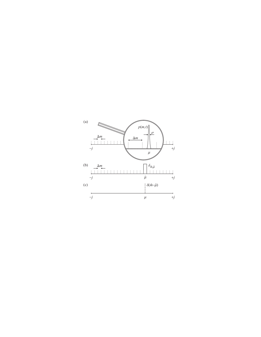
Figure 1: An initial spin-$j$ coherent state $\left|\vartheta_{0},\varphi_{0}\right\rangle$ precesses into the coherent state $\left|\vartheta,\varphi\right\rangle$ at time $t$ under a quantum time evolution. (a) The probability $p(m,t)$ for the outcome $m$ in a measurement of the spin’s $z$-component is given by a Gaussian distribution with width $\sigma$ and mean $\mu$, which can be seen under the magnifying glass of sharp measurements. (b) The measurement resolution $\Delta m$ is finite and subdivides the $2j+1$ possible outcomes into a smaller number of coarse-grained ”slots”. If the measurement accuracy is much poorer than the width $\sigma$, i.e., $\Delta m\gg\!\sqrt{j}$, the sharply peaked Gaussian cannot be distinguished anymore from the discrete Kronecker delta $\delta_{\bar{m},\bar{\mu}}$ where $\bar{m}$ is numbering the slots and $\bar{\mu}$ is the slot in which the center $\mu$ of the Gaussian lies. (c) In the limit $j\rightarrow\infty$ the slots seem to become infinitely narrow and $\delta_{\bar{m},\bar{\mu}}$ becomes the Dirac delta function $\delta(\bar{m}\!-\!\bar{\mu})$.

Under a fuzzy measurement the reduced (projected) state is essentially the state before the measurement. If $\left|\vartheta,\varphi\right\rangle$ is centered well inside the slot, the disturbance is exponentially small. Only in the cases where it is close to the border between two slots, the measurement is invasive. Assuming that the measurement times and/or slot positions chosen by the observer are statistically independent of the (initial) position of the coherent state, a disturbance happens merely in the fraction $\sigma/\Delta m\ll 1$ of all measurements. This is equivalent to the already assumed condition $\!\sqrt{j}\ll\Delta m$. Therefore, fuzzy measurements of a spin coherent state are largely non-invasive such as in any macrorealistic theory, in particular classical Newtonian physics. Small errors may accumulate over many measurements and eventually there might appear deviations from the classical time evolution. This, however, is unavoidable in any explanation of classicality gradually emerging out of quantum theory. To which extent this effect is relevant for our every-day experience is an open issue .

Hence, at the coarse-grained level the physics of the (quantum) spin system can completely be described by a ”new” formalism, utilizing a (classical) spin vector $\mathbf{J}$ at time $t=0$, pointing in the ($\vartheta_{0},\varphi_{0}$)-direction with length $J\equiv|\mathbf{J}|=\!\sqrt{j(j\!+\!1)}\approx j$, where $j\gg 1$, and a (Hamilton) function

$$H=\mathbf{J}^{2}/2I+\omega\,J_{x}\,.$$ (8)

At any time the probability that the spin vector’s $z$-component $J\cos\vartheta\approx j\cos\vartheta$ is in slot $\bar{m}$ is given by $\delta_{\bar{m},\bar{\mu}}$, eq. (6), as if the time evolution of the spin components $J_{i}$ ($i=x,y,z$) is given by the Poisson brackets, $\dot{J}_{i}=[J_{i},H]_{\text{PB}}$, and measurements are non-invasive. Only the term $\omega\,J_{x}$ in eq. (8) governs the time evolution and the solutions correspond to a rotation around the $x$-axis. In the proper continuum limit the spin vector at time $t$ points in the ($\vartheta,\varphi$)-direction where $\vartheta$ and $\varphi$ are the same as for the spin coherent state and the prediction is given by $\delta(\bar{m}\!-\!\bar{\mu})$, eq. (7). This is classical (Newtonian) mechanics.

Finally, we show that the time evolution of any spin-$j$ quantum state becomes classical under the restriction of coarse-grained measurements. At all times any (pure or mixed) spin-$j$ density matrix can be written in the diagonal form Arec1972

$$\hat{\rho}={\displaystyle\iint\nolimits_{\Omega}}\,f(\vartheta,\varphi)\,|\vartheta,\varphi\rangle\langle\vartheta,\varphi|\,\text{d}^{2}\Omega$$ (9)

with d${}^{2}\Omega\equiv\sin\vartheta\,$d$\vartheta\,$d$\varphi$ the infinitesimal solid angle element and $f(\vartheta,\varphi)$—usually known as $P$-function—a not necessarily positive real function (normalization ${\textstyle\iint\nolimits_{\Omega}}\,f(\vartheta,\varphi)\,$d${}^{2}\Omega=1$).

The probability for an outcome $m$ in a $\hat{J}_{z}$ measurement in the state (9) is $P(m)={\textstyle\iint\nolimits_{\Omega}}\,f(\vartheta,\varphi)\,p(m)\,$d${}^{2}\Omega$, where $p(m)$ is given by eq. (5). At the coarse-grained level of classical physics only the probability for a slot outcome $\bar{m}$ can be measured, i.e., $\bar{P}(\bar{m})\equiv{\textstyle\sum\nolimits_{m\in\{\bar{m}\}}}P(m)$ with $\{\bar{m}\}$ the set of all $m$ belonging to $\bar{m}$. For $\Delta m\gg\!\sqrt{j}$ and large $j$ this can be well approximated by

$$\bar{P}(\bar{m})\approx{\displaystyle\int\nolimits_{0}^{2\pi}}\!{\displaystyle\int\nolimits_{\vartheta_{1}(\bar{m})}^{\vartheta_{2}(\bar{m})}}f(\vartheta,\varphi)\sin\vartheta\,\text{d}\vartheta\,\text{d}\varphi\,,$$ (10)

where $\vartheta_{1}(\bar{m})$, $\vartheta_{2}(\bar{m})$ are the borders of the polar angle region corresponding to a projection onto $\bar{m}$. We will show that $\bar{P}(\bar{m})$ can be obtained from a positive probability distribution of classical spin vectors. Consider the function

$$g(\vartheta,\varphi)\equiv\frac{2j+1}{4\,\pi}\,{\displaystyle\iint\nolimits_{\Omega^{\prime}}}\,f(\vartheta^{\prime},\varphi^{\prime})\,\cos^{4j}\!\tfrac{\Theta}{2}\,\,\text{d}^{2}\Omega^{\prime}$$ (11)

with d${}^{2}\Omega^{\prime}\equiv\sin\vartheta^{\prime}\,$d$\vartheta^{\prime}\,$d$\varphi^{\prime}$ and $\Theta$ the angle between the directions $(\vartheta,\varphi)$ and $(\vartheta^{\prime},\varphi^{\prime})$. The distribution $g(\vartheta,\varphi)$ is positive (and normalized) because it is, up to a normalization factor, the expectation value Tr$[\hat{\rho}\,|\vartheta,\varphi\rangle\langle\vartheta,\varphi|]=\langle\vartheta,\varphi|\,\hat{\rho}\,|\vartheta,\varphi\rangle$ of the state $\left|\vartheta,\varphi\right\rangle$. It is usually known as the $Q$-function Agar1981 .

For fuzzy measurements with inaccuracy $\Delta\Theta\sim\vartheta_{2}(\bar{m})-\vartheta_{1}(\bar{m})\gg 1/\!\sqrt{j}$, which is equivalent to $\Delta m\gg\!\sqrt{j}$, the probability for having an outcome $\bar{m}$ can now be expressed only in terms of the positive distribution $g$:

$$\bar{P}(\bar{m})\approx{\displaystyle\int\nolimits_{0}^{2\pi}}\!{\displaystyle\int\nolimits_{\vartheta_{1}(\bar{m})}^{\vartheta_{2}(\bar{m})}}g(\vartheta,\varphi)\sin\vartheta\,\text{d}\vartheta\,\text{d}\varphi\,.$$ (12)

The approximate equivalence of eqs. (10) and (12) is shown by substituting eq. (11) into (12). Note, however, that $g$ is a mere mathematical tool and not experimentally accessible. Operationally, because of $\Delta m\gg\!\sqrt{j}$ an averaged version of $g$, denoted as $h$, is used by the experimenter to describe the system in the classical limit. Mathematically, this function $h$ is obtained by integrating $g$ over solid angle elements corresponding to the measurement inaccuracy. Without the ”magnifying glass” the regions given by the experimenter’s resolution become ”points” on the sphere where $h$ is defined. Thus, a full description is provided by an ensemble of classical spins with the probability distribution $h$.

The time evolution of the general state (9) is determined by (3). In the classical limit it can be described by an ensemble of classical spins characterized by the initial distribution $g$ ($h$), where each spin is rotating according to the Hamilton function (8). From eq. (12) one can see that for the non-invasiveness at the classical level it is the change of the $g$ ($h$) distribution which is important and not the change of the quantum state or equivalently f itself. In fact, upon a fuzzy $\hat{J}_{z}$ measurement the state $\hat{\rho}$ is reduced to one particular state, say to $\hat{\rho}_{\bar{m}}$, with the corresponding (normalized) functions $f_{\bar{m}}$, $g_{\bar{m}}$ and $h_{\bar{m}}$. The reduction to $\hat{\rho}_{\bar{m}}$ happens with probability $\bar{P}(\bar{m})$, which is given by eq. (10) or (12). Whereas the $f$-function can change dramatically upon reduction, $g_{\bar{m}}$ is (up to normalization) approximately the same as $g$ in the region $\Omega_{\bar{m}}$ between two circles of latitude corresponding to the slot $\bar{m}$ and zero outside. If $\hat{Q}_{\bar{m}}\equiv{\textstyle\sum\nolimits_{m\in\{\bar{m}\}}}\left|m\right\rangle\!\left\langle m\right|$ denotes the projector onto the slot $\bar{m}$, then $\hat{Q}_{\bar{m}}\,|\vartheta,\varphi\rangle$ is almost zero ($|\vartheta,\varphi\rangle$) for all coherent states lying outside (inside) $\Omega_{\bar{m}}$. Thus, $g_{\bar{m}}\propto\langle\vartheta,\varphi|\,\hat{\rho}_{\bar{m}}\,|\vartheta,\varphi\rangle\propto\langle\vartheta,\varphi|\,\hat{Q}_{\bar{m}}\,\hat{\rho}\,\hat{Q}_{\bar{m}}\,|\vartheta,\varphi\rangle\approx\langle\vartheta,\varphi|\,\hat{\rho}\,|\vartheta,\varphi\rangle\propto g$ inside and almost zero outside. Hence, at the coarse-grained level the distribution $g_{\bar{m}}$ ($h_{\bar{m}}$) of the reduced state after the measurement can always be understood approximately as a subensemble of the (classical) distribution $g$ before the measurement. Effectively, the measurement only reveals already existing properties in the mixture and does not alter the subsequent time evolution of the individual classical spins.

The disturbance at that level is quantified by how much $g_{\bar{m}}$ differs from a function which is (up to normalization) $g$ within $\Omega_{\bar{m}}$ and zero outside. One may think of dividing all $g$ distributions into two extreme classes, i.e., the ones which show narrow pronounced regions of size comparable to individual coherent states and the ones which change smoothly over regions larger or comparable to the slot size. The former is highly disturbed but in an extremely rare fraction of all measurements. The latter is disturbed in general in a single measurement but to very small extent, as the weight on the slot borders ($\propto\!\!\sqrt{j}$) is small compared to the weight well inside the slot ($\propto\!\Delta m$). (In the intermediate cases one has a trade-off between these two scenarios.) The typical fraction of these weights is $\!\sqrt{j}/\Delta m\ll 1$. Thus, in any case classicality arises with overwhelming statistical weight.

Conclusion.—We showed that the time evolution of an arbitrarily large spin cannot be understood classically, as long as consecutive outcomes in a spin component measurement are resolved. For certain Hamiltonians, given the limitation of coarse-grained measurements, not only is macrorealism valid, but even the Newtonian time evolution of an ensemble of classical spins emerges out of a full quantum description of an arbitrary spin state—even for isolated systems. This suggests that classical physics can be seen as implied by quantum mechanics under the restriction of fuzzy measurements.

We thank M. Aspelmeyer, T. Paterek, M. Paternostro and A. Zeilinger for helpful remarks. This work was supported by the Austrian Science Foundation FWF, the European Commission, Project QAP (No. 015846), and the FWF Doctoral Program CoQuS. J. K. is recipient of a DOC fellowship of the Austrian Academy of Sciences.

References

- (1) J. S. Bell, Physics (New York) 1, 195 (1964).
- (2) A. J. Leggett and A. Garg, Phys. Rev. Lett. 54, 857 (1985); A. J. Leggett, J. Phys.: Cond. Mat. 14, R415 (2002).
- (3) E. Schrödinger, Die Naturwissenschaften 48, 807 (1935).
- (4) W. H. Zurek, Phys. Today 44, 36 (1991); W. H. Zurek, Rev. Mod. Phys. 75, 715 (2003).
- (5) G. C. Ghirardi, A. Rimini, and T. Weber, Phys. Rev. D 34, 470 (1986); R. Penrose, Gen. Rel. Grav. 28, 581 (1996).
- (6) A. Peres, Quantum Theory: Concepts and Methods (Kluwer Academic Publishers, 1995).
- (7) A. Garg and N. D. Mermin, Phys. Rev. Lett. 49, 901 (1982).
- (8) L. G. Yaffe, Rev. Mod. Phys. 54, 407 (1982); K. G. Kay, J. Chem. Phys. 79, 3026 (1983).
- (9) J. M. Radcliffe, J. Phys. A: Gen. Phys. 4, 313 (1971); P. W. Atkins and J. C. Dobson, Proc. R. Soc. A 321, 321 (1971).
- (10) D. Poulin, Phys. Rev. A 71, 022102 (2005); P. Busch, M. Grabowski, and P. J. Lahti, Operational Quantum Physics (Springer, 1995); M. Gell-Mann and J. B. Hartle, Phys. Rev. A 76, 022104 (2007).
- (11) F. T. Arecchi, E. Courtens, R. Gilmore, and H. Thomas, Phys. Rev. A 6, 2211 (1972).
- (12) G. S. Agarwal, Phys. Rev. A 24, 2889 (1981); G. S. Agarwal, Phys. Rev. A 47, 4608 (1993).