Configuration-Space Location of the Entanglement between Two Subsystems

Abstract

In this paper we address the question: where in configuration space is the entanglement between two particles located? We present a thought-experiment, equally applicable to discrete or continuous-variable systems, in which one or both parties makes a preliminary measurement of the state with only enough resolution to determine whether or not the particle resides in a chosen region, before attempting to make use of the entanglement. We argue that this provides an operational answer to the question of how much entanglement was originally located within the chosen region. We illustrate the approach in a spin system, and also in a pair of coupled harmonic oscillators. Our approach is particularly simple to implement for pure states, since in this case the sub-ensemble in which the system is definitely located in the restricted region after the measurement is also pure, and hence its entanglement can be simply characterised by the entropy of the reduced density operators. For our spin example we present results showing how the entanglement varies as a function of the parameters of the initial state; for the continuous case, we find also how it depends on the location and size of the chosen regions. Hence we show that the distribution of entanglement is very different from the distribution of the classical correlations.

I Introduction

Studying the entanglement properties of a number of spatially extended many-body systems including spin chains, coupled fermions, and harmonic oscillators Osborne and Nielsen (2002); Osterloh et al. (2002); Vidal et al. (2003); Latorre et al. (2004); Jin and Korepin (2004); Zanardi and Wang (2002); Martin-Delgado (2002); Audenaert et al. (2002); Plenio et al. (2004); Vedral (2003) has both given information on the potential uses of these systems in quantum information processing, and yielded insight into their fundamental properties. Quantum entanglement is a measure of essentially quantum correlations, and many interacting systems possess an entangled ground state Nielsen (1998); Wootters (2002a, b); O’Connor and Wootters (2001); Osborne and Nielsen (2002); Osterloh et al. (2002); Briegel and Raussendorf (2001).

In this paper we address the question: where in configuration space is the entanglement between two particles located? We pose the question using the language of spatial entanglement, which plays a significant role in many physical realizations of QIP (quantum information processing). However our results are easily recast in terms of other types of entanglement. Specifically, we investigate the location dependence of the ground-state entanglement between two interacting subsystems. We choose a pair of coupled harmonic oscillators as an example, since this is a system for which many exact results are available Audenaert et al. (2002); Giedke et al. (2003). We assign one oscillator to each of the two communicating parties Alice and Bob, but perform a thought experiment in which one or both of them first measure the system in configuration space, with just enough precision to localise it in some chosen region, and thereafter are restricted to operations only within that region. This restriction corresponds to a particular type of projective filtering in configuration space. We ask how this restriction affects the spatial entanglement available to them for other purposes—for example, for teleporting additional qubits between them. This should be distinguished from the approach taken recently by Cavalcanti et. al. Cavalcanti et al. (2005), who explored the effect of a finite-resolution spatial measurement on the spin entanglement of a system of noninteracting fermions and also a photonic interferometer. Our research also contrasts with previous studies Botero and Reznik (2004); Plenio et al. (2005); Heaney et al. (2006) of the entanglement of a finite region of space with the rest of the system.

In a previous paper Lin and Fisher (2006) we investigated the limiting case where the size of the preliminary-measurement region is very small, and showed that a smooth two-mode continuous-variable state can be approximated by a pair of qubits and its entanglement fully characterized, even for mixed states, by either concurrence density or negativity density; here we shall focus on studying the variations of the entanglement properties with the size of the region. For the present we assume that the two particles are distinguishable; the effects of indistinguishability on the phenomena discussed here are a subject for further work. We argue that the shared entanglement remaining to Alice and Bob provides a natural measure of where in configuration space the entanglement was originally located. We show that the distribution of entanglement is very different from that of the classical correlations.

II Theory

II.1 Restricting configuration space by Von Neumann measurements

Let the configuration space of the whole system be described by the coordinates $q_{A}$ and $q_{B}$, where $q_{A}$ describes Alice’s particle and $q_{B}$ describes Bob’s. We will initially present the case in which only Alice makes a preparatory measurement on her system; suppose she has access to some restricted portion $\mathcal{A}$ of the configuration space of “her” particle, whose coordinate is $q_{A}$. If she measures her system with just enough accuracy to determine whether it is in region $\mathcal{A}$ or not, but no more, the effect is to localise the wavefunction either inside, or outside, the chosen region. The restriction to lying inside the region corresponds to the projector

$$\hat{E}_{\mathcal{A}}=\int_{\mathcal{A}}\left|q_{A}\right\rangle\left\langle q_{A}\right|\mathrm{d}q_{A}\otimes\hat{1}_{\mathrm{other}},$$ (1)

where $\hat{1}_{\mathrm{other}}$ is the identity operation for all the other particles (assumed distinguishable) in the system.

II.1.1 The discarding ensemble

Suppose $\mathcal{A}$ is of finite extent, and Alice measures the position of her particle with just enough accuracy to determine whether it is in $\mathcal{A}$ or not. If so, she keeps the state for further use; if not, she discards it (and tells Bob she has done so). Then the density matrix appropriate to the ensemble of retained systems is

$$\hat{\rho}_{D,\mathcal{A}} = \frac{\hat{E}_{\mathcal{A}}\hat{\rho}\hat{E}_{\mathcal{A}}}{\mathrm{Tr}(\hat{E}_{\mathcal{A}}\hat{\rho})}$$

$$= \frac{\theta_{\mathcal{A}}(q_{A})\rho(q_{A},q_{\mathrm{other}};q^{\prime}_{A},q^{\prime}_{\mathrm{other}})\theta_{\mathcal{A}}(q^{\prime}_{A})}{\int\int_{\mathcal{A}}\rho(q_{A},q_{\mathrm{other}};q_{A},q_{\mathrm{other}})\mathrm{d}q_{A}\mathrm{d}q_{\mathrm{other}}},$$

where $\theta_{\mathcal{A}}$ is a generalized Heavyside function defined so that

$$\theta_{\mathcal{A}}(q)=\left\{\begin{array}[]{l}1\quad\mathrm{if}\,q\in\mathcal{A}\\ 0\quad\mathrm{otherwise}\end{array}\right..$$ (3)

The subscript $D$ refers to the discarding of the unwanted states; we refer to this density matrix as describing the “discarding ensemble”. Note that, if the original $\hat{\rho}$ was a pure state $\left|\psi\right\rangle\left\langle\psi\right|$, then the post-selected density matrix is also pure:

$$\hat{\rho}_{D,\mathcal{A}}=\frac{\hat{E}_{\mathcal{A}}\left|\psi\right\rangle\left\langle\psi\right|\hat{E}_{\mathcal{A}}}{\left\langle\psi\right|\hat{E}_{\mathcal{A}}\left|\psi\right\rangle}.$$ (4)

In particular this means that even though the system has continuous variables and is therefore infinite-dimensional, its entanglement $\mathcal{E}_{D,\mathcal{A}}$ is easily calculated through the von Neumann entropy $S(\hat{\rho}^{(A)})$ of the reduced density matrix $\hat{\rho}^{(A)}=\mathrm{Tr}_{B}\hat{\rho}$.

II.1.2 The non-discarding ensemble

On the other hand if Alice chooses not to discard the system when she fails to detect a particle in region $\mathcal{A}$, the appropriate density matrix is

$$\hat{\rho}_{ND}=\hat{E}_{\mathcal{A}}\hat{\rho}\hat{E}_{\mathcal{A}}+\hat{E}_{\mathcal{A}^{\prime}}\hat{\rho}\hat{E}_{\mathcal{A}^{\prime}},$$ (5)

where the subscript $ND$ refers to “non-discarding” and the complementary projector $\hat{E}_{\mathcal{A}^{\prime}}$ is defined as

$$\hat{E}_{\mathcal{A}^{\prime}}\equiv\hat{1}-\hat{E}_{\mathcal{A}}=\int_{q_{A}\notin\mathcal{A}}\left|q_{A}\right\rangle\left\langle q_{A}\right|\mathrm{d}q_{A}\otimes\hat{1}_{\mathrm{other}}.$$ (6)

Eq. (5) describes a mixed state. It differs from the original density matrix $\hat{\rho}$ in that off-diagonal elements of $\hat{\rho}$ connecting $q_{A}\in\mathcal{A}$ and $q_{A}\notin\mathcal{A}$ have been set to zero.

Let $p_{\mathcal{A}}=\mathrm{Tr}[\hat{E}_{\mathcal{A}}\hat{\rho}\hat{E}_{\mathcal{A}}]$ be the probability of finding Alice’s particle in $\mathcal{A}$. Since the first and second components of $\hat{\rho}_{ND}$ can be distinguished by Alice and Bob using local operations and classical communication (LOCC), they can teleport $p_{\mathcal{A}}\mathcal{E}_{D,\mathcal{A}}+(1-p_{\mathcal{A}})\mathcal{E}_{D,\mathcal{A^{\prime}}}$ qubits on average between them. Hence the distallable entanglement (and therefore also the entanglement of formation) of $\hat{\rho}_{ND}$ is not less than $p_{\mathcal{A}}\mathcal{E}_{D,\mathcal{A}}+(1-p_{\mathcal{A}})\mathcal{E}_{D,\mathcal{A^{\prime}}}$. On the other hand, Eq. (5) also constitutes a valid decomposition of the non-discarding density matrix $\hat{\rho}_{ND}$ into orthogonal pure states; it follows that the entanglement of formation $\mathcal{E}_{ND}$ is not greater than the average entanglement of this decomposition: $\mathcal{E}_{ND}\leq p_{\mathcal{A}}\mathcal{E}_{D,\mathcal{A}}+(1-p_{\mathcal{A}})\mathcal{E}_{D,\mathcal{A^{\prime}}}$. The only way these two observations can be consistent is if

$$\mathcal{E}_{ND}=p_{\mathcal{A}}\mathcal{E}_{D,\mathcal{A}}+(1-p_{\mathcal{A}})\mathcal{E}_{D,\mathcal{A^{\prime}}}.$$ (7)

If all the operators available to Alice have support only in region $\mathcal{A}$ (i.e. if she can neither measure her particle’s properties, or manipulate it in any way, except when it is in $\mathcal{A}$) then the component projected by $\hat{E}_{\mathcal{A}^{\prime}}$ is “out of reach”, and the second component $\hat{E}_{\mathcal{A}^{\prime}}\hat{\rho}\hat{E}_{\mathcal{A}^{\prime}}$ of the state $\hat{\rho}_{ND}$ is functionally equivalent to a separable state as far as any operation that Alice and Bob can perform is concerned. It does not possess any entanglement properties that are useful to Alice and Bob. In that case, Eq.  (7) reduces to $\mathcal{E}_{ND}=p_{\mathcal{A}}\mathcal{E}_{D,\mathcal{A}}$.

II.1.3 Precise measurements of position

If, on the other hand, Alice measures the position accurately, but again keeps only those occasions when the results lie within $\mathcal{A}$, the discarding ensemble’s density matrix is

$$\hat{\rho}_{P}=\frac{\int_{\mathcal{A}}\hat{E}_{q}\hat{\rho}\hat{E}_{q}\mathrm{d}q}{\int_{\mathcal{A}}\mathrm{Tr}(\hat{E}_{q}\hat{\rho})\mathrm{d}q},$$ (8)

where the subscript $P$ refers to measuring precisely and $\hat{E}_{q}$ is the projector corresponding to measuring Alice’s particle $A$ precisely at position $q$:

$$\hat{E}_{q}=\delta(q_{A}-q).$$ (9)

Eq. (8) describes a density matrix that is diagonal in $q_{A}$; it is a mixed state even if all the measurements where the particle is not found in $\mathcal{A}$ are discarded. Furthermore, unless there are some additional degrees of freedom of particle $q_{A}$ which are not measured, the overall density matrix can be written as an incoherent sum of product states:

$$\hat{\rho}_{P} = \int_{\mathcal{A}}\hat{E}_{q}\hat{\rho}\hat{E}_{q}\mathrm{d}q$$ (10)

$$= \int_{\mathcal{A}}\left|q_{A}\right\rangle\left\langle q_{A}\right|\mathrm{d}q_{A},$$

where $|q_{A}\rangle$ is a state in which particle A is located exactly at $q_{A}$ and particle B is in some arbitrary state. $\hat{\rho}_{P}$ therefore contains no remaining entanglement with Bob’s particle B.

Note that in the limit of very small measurement regions, the distinction between precise and imprecise measurements disappears. The case of vanishingly small regions was analysed in a previous paper Lin and Fisher (2006), where it was shown that a well-defined concurrence density exists, and so the concurrence after the measurement is directly proportional to the region size.

II.1.4 Measurements by both parties

Exactly analogous formulae can be written down for the cases where Bob makes a preliminary measurement on his particle, or both partners make a measurement. In the case where both parties make a preliminary measurement, the reduced density matrix of Alice’s system that is used to calculate the entanglement will naturally depend also on the measurement performed by Bob.

II.1.5 An inequality for the discarding entanglement

Suppose Alice and Bob divide their configuration spaces into a set of segments $\mathcal{A}$ and $\mathcal{B}$ respectively, and each make a measurement determining in which segment the system is located. In the nondiscarding ensemble, Eq. (5) generalizes to

$$\hat{\rho}_{ND}=\sum_{\mathcal{AB}}\hat{E}_{\mathcal{B}}\hat{E}_{\mathcal{A}}\hat{\rho}\hat{E}_{\mathcal{A}}\hat{E}_{\mathcal{B}},$$ (11)

where

$$\sum_{\mathcal{A}}\hat{E}_{\mathcal{A}}=\sum_{\mathcal{B}}\hat{E}_{\mathcal{B}}=\hat{1}.$$ (12)

However, this corresponds to a local operation performed by Alice and Bob. Their shared entanglement is non-increasing under this operation; therefore,

$$\mathcal{E}(\hat{\rho})\geq\mathcal{E}(\hat{\rho}_{ND}).$$ (13)

But, by a straightforward extension of the argument given above,

$$\mathcal{E}(\hat{\rho}_{ND})=\sum_{\mathcal{AB}}p_{\mathcal{AB}}\mathcal{E}_{D}(\hat{\rho}_{D,\mathcal{A}\mathcal{B}}),$$ (14)

where

$$p_{\mathcal{AB}}=\mathrm{Tr}[\hat{E}_{\mathcal{B}}\hat{E}_{\mathcal{A}}\hat{\rho}]$$ (15)

is the probability of finding Alice’s part of the system in $\mathcal{A}$ and Bob’s part in $\mathcal{B}$, and

$$\hat{\rho}_{D,\mathcal{A}\mathcal{B}}=\frac{\hat{E}_{\mathcal{B}}\hat{E}_{\mathcal{A}}\hat{\rho}\hat{E}_{\mathcal{A}}\hat{E}_{\mathcal{B}}}{p_{\mathcal{AB}}}$$ (16)

is the density matrix in the discarding ensemble after this measurement result has been obtained. Combining Eq. (13) and Eq. (14) we obtain the following inequality for the average of the entanglement in the discarding ensemble over all the partitions:

$$\sum_{\mathcal{AB}}p_{\mathcal{AB}}\mathcal{E}_{D}(\hat{\rho}_{D,\mathcal{A}\mathcal{B}})\leq\mathcal{E}(\hat{\rho}).$$ (17)

II.2 Spin systems

We can make an exactly analogous theory for the case where Alice and Bob share a system defined on some other state space, for example a spin system—perhaps more familiar in quantum information theory. We simply replace the projection operator $\hat{E}_{\mathcal{A}}$ by one defined in spin space; for example, $\hat{E}_{\mathcal{A}}$ might project onto states with a specified spin component in a given direction. The rest of the theory is as outlined above.

III The physical systems

III.1 Spins

Suppose that both Alice and Bob each possess two spins; the first spins belonging to each of them are entangled, as are the second spins, and the overall state $\left|\psi\right\rangle$ of the system is a product of the state of the two pairs. For example, we could write

$$\left|\psi\right\rangle = (\cos\theta_{1}\left|\uparrow_{A1}\uparrow_{B1}\right\rangle+\sin\theta_{1}\left|\downarrow_{A1}\downarrow_{B1}\right\rangle)$$ (18)

$$\quad\otimes(\cos\theta_{2}\left|\uparrow_{A2}\uparrow_{B2}\right\rangle+\sin\theta_{2}\left|\downarrow_{A2}\downarrow_{B2}\right\rangle);$$

the state is pure so entanglement between Alice’s and Bob’s subsystems is well quantified by the von Neumann entropy of the reduced density matrix. Suppose also that Alice and Bob can only handle systems if the total spins $M_{s}$ available to each party are such that $M_{s}=0$; perhaps the parts of the state with non-zero moment are lost because of the presence of large fluctuating fields in the environment. In the discarding ensemble defined by this restriction, the state becomes

$$\left|\psi\right\rangle_{R} = \frac{1}{\sqrt{1-\cos 2\theta_{1}\cos 2\theta_{2}}}$$ (19)

$$\quad(\cos\theta_{1}\left|\uparrow_{A1}\uparrow_{B1}\right\rangle\sin\theta_{2}\left|\downarrow_{A2}\downarrow_{B2}\right\rangle$$

$$\quad+\sin\theta_{1}\left|\downarrow_{A1}\downarrow_{B1}\right\rangle\cos\theta_{2}\left|\uparrow_{A2}\uparrow_{B2}\right\rangle),$$

again this restricted state is pure but entanglement should become quite different.

This type of measurement is familar in other contexts—for example entanglement distillation and concentration Bennett et al. (1996a, b).

Entanglement of a bi-partite mixed spin state can also be easily quantified by using negativity $\mathcal{N}(\hat{\rho})$ instead as the entanglement measure. We define negativity as the sum of the magnitudes of the negative eigenvalues $\lambda_{i}$ of the partially transposed density matrix $\hat{\rho}^{T_{B}}$,

$$\mathcal{N}(\hat{\rho})=\sum_{i\,\textbf{s.t.}\,\lambda_{i}<0}|\lambda_{i}|.$$ (20)

Consider the mixed state defined by

$$\hat{\rho}=\frac{16F-1}{15}\left|\psi\right\rangle\left\langle\psi\right|+\frac{1-F}{15}\hat{1},$$ (21)

where $\left|\psi\right\rangle$ is as defined in Eq. (18) (in contrast to the definition of Werner states, this is not a maximally entangled state) and $F\in[1/16,1]$. Note that when $F=1$, the state becomes pure. Again an example of discarding ensembles can be obtained by projecting the state (21) onto $M_{s}=0$ subspace and renormalizing accordingly.

III.2 Harmonic oscillators

The density matrix of a Gaussian state can be written in the coordinate representation Simon et al. (1987) as

$$\left\langle q\left|\hat{\rho}\right|q^{\prime}\right\rangle \equiv \rho(q;q^{\prime})$$ (22)

$$= \zeta_{1}\mathrm{exp}[-q^{T}\mathbf{L}q-q^{\prime T}\mathbf{L}q^{\prime}$$

$$\qquad-\frac{1}{2}(q-q^{\prime})^{T}\mathbf{M}(q-q^{\prime})$$

$$\qquad+\frac{i}{2}(q-q^{\prime})^{T}\mathbf{K}(q+q^{\prime})],$$

where $\zeta_{1}$ is a normalization constant, and where $\mathbf{L},$ $\mathbf{M}$ and $\mathbf{K}$ are real $N$-dimensional matrices with $\mathbf{L}$ and $\mathbf{M}$ symmetric, while $\mathbf{K}$ is arbitrary. These matrices are related to the covariance matrix $\gamma$ by

$$\frac{1}{2}\gamma^{-1}=\left(\begin{array}[]{cc}\bm{1}&0\\ -\mathbf{K}&\bm{1}\end{array}\right)^{T}\left(\begin{array}[]{cc}2\mathbf{L}&0\\ 0&\frac{1}{2}(\mathbf{L}+\mathbf{M})^{-1}\end{array}\right)\left(\begin{array}[]{cc}\bm{1}&0\\ -\mathbf{K}&\bm{1}\end{array}\right).$$ (23)

We note that for a pure state, $\mathbf{M}=0$ and $\mathbf{K}$ is symmetric.

Consider a harmonic system with a Hamiltonian (taking $\hbar=1$)

$$\hat{H}=R^{T}(\begin{array}[]{cc}\mathbf{V}m\omega^{2}/2&0\\ 0&\bm{1}_{N}/(2m)\end{array})R,$$ (24)

where the vector $R$ of quadrature operators is given by the positions $R_{j}=\hat{X}_{j}$ and conjugate momenta $R_{N+j}=\hat{P}_{j},$ for $1\leq j\leq N,$, the $N\times N$ matrix $\mathbf{V}$ contains the coupling coefficients, and $\omega$ is the natural frequency of uncoupled oscillators. For a translationally invariant system the potential matrix elements depend only on the difference between the indices: $\mathbf{V}_{j,k}=v_{(j-k)\mathrm{mod\,}N}$ for $1\leq j,k\leq N$. The covariance matrix of the ground state is then Audenaert et al. (2002)

$$\gamma = \frac{1}{2}(\frac{\gamma_{x}}{m\omega}\oplus m\omega\gamma_{p})$$ (25)

$$= \frac{1}{2}(\frac{\mathbf{V}^{-1/2}}{m\omega}\oplus m\omega\mathbf{V}^{1/2}).$$

Since the Hamiltonian given in Eq. (24) has no coupling between position and momentum variables, $\gamma$ is block diagonal and hence $\mathbf{K}=0$. Furthermore if there are only nearest-neighbour interactions, with a Hooke’s-law spring constant $K$, the interaction strength is characterized by the single dimensionless parameter

$$\alpha=\frac{2K}{m\omega^{2}}.$$ (26)

For the two-oscillator ground state we therefore have only one non-zero matrix:

$$\mathbf{L}=\frac{m\omega}{8}\left(\begin{array}[]{cc}1+\sqrt{1+4\alpha}&1-\sqrt{1+4\alpha}\\ 1-\sqrt{1+4\alpha}&1+\sqrt{1+4\alpha}\end{array}\right).$$ (27)

The 1-particle reduced density matrices can then be easily obtained by quadrature; for Particle 1,

$$\hat{\rho}^{(A)}(q_{A};q_{A}^{\prime}) = \int_{-\infty}^{\infty}\mathrm{d}q_{B}\rho(q_{A},q_{B};q_{A}^{\prime},q_{B})$$

$$= \sqrt{\frac{2C_{1}-2C_{2}}{\pi}}$$

$$\quad\mathrm{exp}[-C_{1}(q_{A}^{2}+q_{A}^{\prime 2})+2C_{2}q_{A}q_{A}^{\prime}],$$

where the state is normalized to unity and the constants $C_{1}$ and $C_{2}$ are

$$C_{1}=\frac{1+2\alpha+3\sqrt{1+4\alpha}}{8+8\sqrt{1+4\alpha}}m\omega$$ (29)

and

$$C_{2}=\frac{\alpha(\sqrt{1+4\alpha}-1)}{8(1+2\alpha+\sqrt{1+4\alpha})}m\omega.$$ (30)

From Eq. (III.2), we can also define the Gaussian characteristic length $\sigma$ which characterizes the probability distribution of a single particle:

$$\sigma=\left[2m\omega\left(\frac{\sqrt{1+4\alpha}}{1+1\sqrt{1+4\alpha}}\right)\right]^{-\frac{1}{2}}.$$ (31)

For bipartite Gaussian states, the entanglement of formation is known exactly Rendell and Rajagopal (2005). For the ground state of our system, the value is

$$S(\hat{\rho}^{(A)})=-\log_{2}{(1-w)}-\frac{w\log_{2}w}{(1-w)},$$ (32)

where

$$w=\frac{1+3\,{\sqrt{1+4\,\alpha}}+2\,[\alpha-\,{\left(1+4\,\alpha\right)}^{\frac{1}{4}}-\,{\left(1+4\,\alpha\right)}^{\frac{3}{4}}]}{1+2\,\alpha-{\sqrt{1+4\,\alpha}}}.$$ (33)

IV Method

For the spin system, the entanglement can be calculated straightforwardly by standard methods; for the two-oscillator system, we calculate the von Neumann entropy $S(\hat{\rho}^{(A)})$, and hence the entanglement, numerically by using two different approaches.

IV.1 Expansion in a complete set

We define an orthonormal set of functions, $\{\phi_{n}(q)\}$, with support in a region $\mathcal{A}$ of configuration space of width $2a$ centred at coordinate $\bar{q}$:

$$\int_{\bar{q}-a}^{\bar{q}+a}\phi_{n}(q)\phi_{m}^{*}(q)=\delta_{nm}.$$ (34)

A suitable choice is

$$\phi_{n}(q) = \sqrt{\frac{1}{a}}\cos(\frac{(q-\bar{q})n\pi}{2a})\quad\textrm{$n$ is odd}$$

$$\phi_{n}(q) = \sqrt{\frac{1}{a}}\sin(\frac{(q-\bar{q})n\pi}{2a})\quad\textrm{$n$ is even},$$

$$= 0\quad\textrm{if}\quad\left|q-\bar{q}\right|>a$$

We then approximate the appropriate post-selected density matrix by an expansion in a finite set of the functions defined in Eq. (IV.1); as an example, if only Alice makes a preliminary measurement to localise her particle in the region $\mathcal{A}$, we have:

$$\hat{\rho}^{(A)}_{D}(q_{A};q_{A}^{\prime})=\sum_{mn}^{N}\rho_{mn}\phi_{m}(q_{A})\phi_{n}^{*}(q_{A}^{\prime}),$$ (36)

with $\rho_{mn}$ given by

$$\rho_{mn} = \int_{\bar{q}_{A}-a}^{\bar{q}_{A}+a}\mathrm{d}q_{A}\int_{\bar{q}_{A}-a}^{\bar{q}_{A}+a}\mathrm{d}q_{A}^{\prime}$$ (37)

$$\quad\phi_{m}^{*}(q_{A})\hat{\rho}^{(A)}(q_{A};q_{A}^{\prime})\phi_{n}(q_{A}^{\prime}),$$

where $\hat{\rho}^{(A)}(q_{A};q_{A}^{\prime})$ is Eq. (III.2). We normalize $\hat{\rho}^{(A)}_{D}(q_{A};q_{A}^{\prime})$ by its trace and can then quantify entanglement by calculating the von Neumann entropy from this normalized $\hat{\rho}^{(A)}_{D}(q_{A};q_{A}^{\prime})$. Unfortunately the quadratures in Eq. (37) must be performed numerically, making this approach relatively time-consuming.

IV.2 Configuration-space grid

We therefore explored also a direct real-space approach, in which we first discretize the configuration space into a finite number of measurement “bins”, then select only those bins that correspond to the regions within which Alice’s and Bob’s respective particles localise. For example, consider again the case in which only Alice makes a preliminary measurement, if the region is $\bar{q}_{A}-a\leq q_{A}\leq\bar{q}_{A}+a$, we divide this space into $N_{B}$ regions with $N_{B}+1$ equally spaced points ($q_{A}$’s) covering the intervals from $q_{A}=\bar{q}_{A}-a$ to $\bar{q}_{A}+a$. We then build the $(N_{B}+1)\times(N_{B}+1)$ post-selected 1-particle reduced density matrix $\hat{\rho}^{(A)}_{D}(q_{A};q_{A}^{\prime})$ by calculating its elements $\rho_{mn}$’s from the 1-particle reduced density matrix Eq. (III.2):

$$\rho_{mn}=\hat{\rho}^{(A)}(q_{A}^{m};q_{A}^{n})\quad\mathrm{for}\quad 1\leq m,n\leq N_{B}+1.$$ (38)

As in the other approach, we calculate the von Neumann entropy of the normalized $\hat{\rho}^{(A)}_{D}(q_{A};q_{A}^{\prime})$ in order to quantify the entanglement.

Note that if on the other hand both parties make a preliminary measurement, we start from the full 2-particle density matrix and apply Bob’s restrictions w.r.t his oscillator before we reduce it into the 1-particle density matrix for Alice’s oscillator.

We find that results from the two approaches converge to the same values as the number of grid points, or the number of expansion functions, tend to infinity. Since the second (grid-based) approach is much more efficient to compute, it has been used for all the results presented in this paper.

V Results

V.1 The spin system

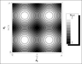
(a) Unrestricted

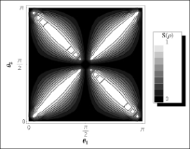
(b) Restricted (discarding ensemble)

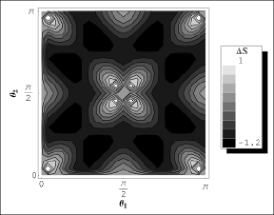
(c) Differences

Figure 1: Entanglement (von Neumann entropy $S(\hat{\rho}^{(A)})$) present in the chosen spin system (a) when the total spins $M_{s}$ is unrestricted, (b) in the discarding ensemble when $M_{s}$ for each party must be 0. (c) Entanglement differences between the two cases; $\Delta S=S(\hat{\rho}^{(A)}_{D})-S(\hat{\rho}^{(A)})$.

(A) $F=0.3$

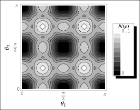
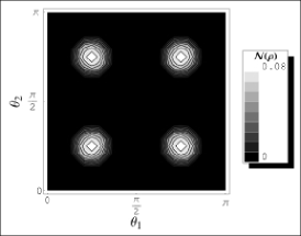
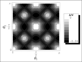
(B) $F=0.65$

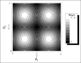
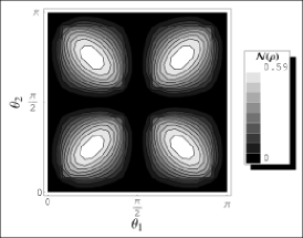
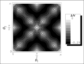
(C) $F=1.0$

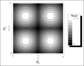
(a) Unrestricted

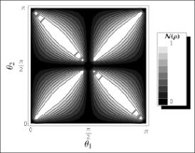
(b) Restricted (discarding ensemble)

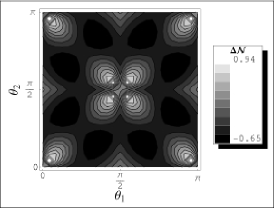
(c) Differences

Figure 2: Entanglement (negativity $\mathcal{N}(\hat{\rho})$) present in the mixed state (21) (a) when the total spins $M_{s}$ is unrestricted, (b) in the discarding ensemble when $M_{s}$ for each party must be 0. (c) Entanglement differences between the two cases; $\Delta\mathcal{N}=\mathcal{N}(\hat{\rho}_{D})-\mathcal{N}(\hat{\rho}_{o})$. $F$ determines the “mixedness” of the state; when $F=1$, the state is pure.

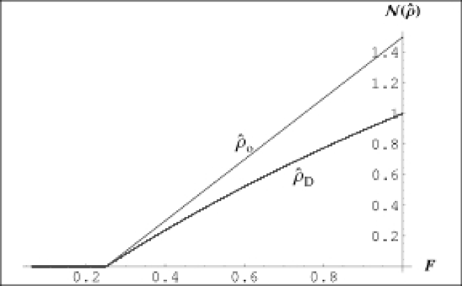
Figure 3: Variation of the entanglement (negativity $\mathcal{N}(\hat{\rho})$) with $F\in[1/16,1]$. $F$ is a quantity that determines the mixedness of the state as defined by Eq. (21). The solid line is for the original ensemble $\hat{\rho}_{o}$ whereas the dashed line is for the corresponding discarding ensemble $\hat{\rho}_{D}$. Both $\theta_{1}$ and $\theta_{2}$ have been set to $\pi/4$ to produce the plots.

V.1.1 Pure states

We present results in Fig. 1. For the spin system we consider, entanglement present in the state Eq. (18) depends on $\theta_{1}$ and $\theta_{2}$ with periods of $\pi/2$, as shown in Fig. 1(a). The maximum entanglement is 2 ebits and occurs when both pairs of spins are in the Bell state ($\theta_{1}=\theta_{2}=(2n+1)\pi/4$). When $\theta_{1}=\theta_{2}=n\pi/2$, the state reduces to all spins either all up or down so completely loses any entanglement.

Now if the restricted region for both Alice and Bob is chosen to be the subspace in which the total $z$-component of spin takes the value zero, and we work in the discarding ensemble so all other states are eliminated, the entanglement properties of the system become very different. Fig. 1(b) shows that the entanglement distribution of the restricted state has periods of $\pi$ instead of $\pi/2$, and the maximum possible entanglement (now 1 ebit since the restricted subspaces for both Alice and Bob are two-dimensional) is achieved whenever $\theta_{1}=\theta_{2}$ or $\theta_{1}+\theta_{2}$ are integer multiples of $\pi$ so that the restricted state is in the Bell state. Note that there is a singularity whenever $\cos 2\theta_{1}\cos 2\theta_{2}=1$.

If we compare Fig. 1(a) and Fig. 1(b), it seems that in some instances the restricted state has higher entanglement. This is indeed the case as shown in Fig. 1(c), where $\Delta S=S(\hat{\rho}^{(A)}_{D})-S(\hat{\rho}^{(A)})$ is plotted against both $\theta_{1}$ and $\theta_{2}$. This is an example of the familiar process of entanglement concentration Bennett et al. (1996a, b), in which some partial entanglement is concentrated after chosen local measurements. Entanglement is not created on average in our example because the probability of finding $M_{s}=0$ is not 100%. Therefore the inequality Eq. (17) is not violated.

V.1.2 Mixed states

Now we perform a similar calculation for the mixed state (21), comparing the entanglement (as quantified by the negativity) present when the total spins $M_{s}$ is unrestricted and the entanglement in the discarding ensemble when $M_{s}$ for each party must be 0. The results are presented in Fig. 2. We choose three values of $F$ for comparison; $F=0.3,$ $F=0.65$ and $F=1$.

In Fig. 3, we plot the variation of the entanglement $\mathcal{N}(\hat{\rho})$ with $F$ by choosing both $\theta_{1}$ and $\theta_{2}$ to be $\pi/4$ (other values can be chosen without affecting the qualitative behaviour but entanglement will not vanish at smaller values of $F$). The case when the total $M_{s}$ is unrestricted $\hat{\rho}_{o}$ is plotted as a solid line, while the case of the corresponding discarding ensemble $\hat{\rho}_{D}$ is plotted as a dashed line. The entanglement in both cases vanishes at $F=0.25$. This is similar to what we observed in a previous paper Lin and Fisher (2006): in that case, we showed that the entanglement (as quantified by the negativity) of a two-mode Gaussian thermal state vanishes at the same temperature regardless of whether the initial state, or the post-selected state in the discarding ensemble, is studied.

V.2 Two oscillators: the limit of small region sizes

For the Gaussian system described in Section III.2 the entanglement can be evaulated analytically in the limit of very small region sizes, following the method described in Lin and Fisher (2006).

V.2.1 Only Alice’s particle restricted

Suppose only Alice makes a preliminary measurement, and determines that her particle is located in a region of length $2a$ centred at coordinate $\bar{q}_{A}$, as in §IV: $\bar{q}_{A}-a\leq q_{A}\leq\bar{q}_{A}+a$. In the discarding ensemble, the entanglement is $E_{D}=h(\epsilon)\equiv-[\epsilon\log_{2}(\epsilon)+(1-\epsilon)\log_{2}(1-\epsilon)]$ with

$$\epsilon=a^{2}m\omega\frac{\alpha(\sqrt{1+4\alpha}-1)}{12(1+2\alpha+\sqrt{1+4\alpha})}.$$ (39)

Note that this depends only on $a$ and on the parameters of the underlying oscillator system; it is independent of $\bar{q}$. Note also that the entanglement is non-zero for any non-zero $\alpha$, and can be made arbitrarily large (for a given small $a$) by increasing $\alpha$.

V.2.2 Both particles restricted

On the other hand, if both parties make measurements, thereby also restricting Bob’s particle to a region of length $2b$ around $\bar{q}_{B}$, the entanglement is once again $h(\epsilon)$ but now $\epsilon$ becomes

$$\epsilon=\frac{a^{2}b^{2}m^{2}\omega^{2}}{72}(1+2\alpha-\sqrt{1+4\alpha}),$$ (40)

and the concurrence density Lin and Fisher (2006) is

$$\frac{\sqrt{2}m\omega}{6}\sqrt{1+2\alpha-\sqrt{1+4\alpha}}$$ (41)

Once again, this result depends only on the dimensionless coupling strength $\alpha$ and the fundamental length unit $(m\omega)^{-1/2}$ of the oscillators; it is again independent of the location of the centres of the measurement regions. Later we will see that as $a$ and $b$ increase, the entanglement distribution gradually changes so that more entanglement is located at some parts of configuration space than the others.

V.3 Two oscillators: finite region sizes

V.3.1 Only Alice’s particle restricted

For simplicity, we will set $m=1$, $\omega=1$ and choose the Gaussian characteristic length (Eq. (31)) for an uncoupled harmonic system, $\sigma=1$, as our unit of length.

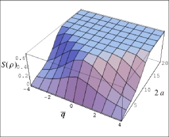
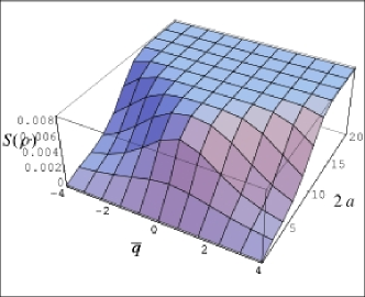
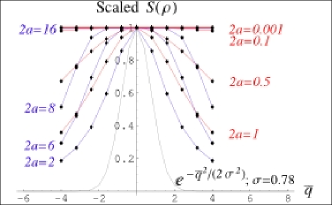
(a) $\alpha=6$

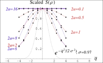
(b) $\alpha=0.06$

Figure 4: (Color online) Top: Variation of the entanglement $S(\hat{\rho}^{(A)})$ with both the width $2a$ and the centre $\bar{q}$ of the preliminary-measurement region. Bottom: $S(\hat{\rho}^{(A)})$ plotted against $\bar{q}$ for different widths, re-scaled such that $S(\hat{\rho}^{(A)})$ has the same peak value at $\bar{q}=0$. A plot (the black dashed line) of the corresponding Gaussian probability distribution for Alice’s particle, with a standard deviation $\sigma$ determined by the coupling strength $\alpha$, is shown for comparison. The different plots correspond to two different coupling strengths, (a) $\alpha=6$ v.s. (b) $\alpha=0.06$. The number of bins $N_{B}$ used in the calculation was 200 in both cases.

In this section, we consider the case in which only Alice makes a preliminary measurement to determine that her particle lies within a finite-size region. Suppose that the size of this region is $2a$ and the location of the centre of the region is $\bar{q}$, the von Neumann entropy $S(\hat{\rho}^{(A)})$ depends on both $2a$ and $\bar{q}$. This is shown in Fig. 4. We look at the variation with $\bar{q}$ first; Fig. 4 along the $\bar{q}$-axis shows some of the examples. For finite $a$, the entanglement is higher if we measure around the centre of the wavefunction, where the probability of finding a particle is highest, than if we take our measurements further away from the the centre of the wavefunction where the chance of finding a particle is very low.

We can understand this variation by examining Alice’s post-selected reduced density matrix in the centre of Fig. 4 ($\bar{q}=0$) and at the edge ($\bar{q}=\pm 4$). At the edge, the diagonal elements increase rapidly towards one end; the eigenvalues of this density matrix are dominated by these terms, resulting in one eigenvalue being close to 1 and the other eigenvalues being very small. The von Neumann entropy will therefore also be small. In contrast, the diagonal elements in the centre case, instead of being dominated by a single element at one end, are approximately constant. The resulting spread of eigenvalues leads to a higher von Neumann entropy.

We would also expect that as the region size approaches the total configuration space, the entanglement in the discarding ensemble should tend to the entanglement originally present in the whole system; this is shown in the upper part of Fig. 4, where the entanglement rises with $a$ until it saturates to the peak value of magnitude $S(\hat{\rho}^{(A)})=0.702$ given by Eq. (32). Roughly speaking, this saturation occurs once the region has expanded to include a significant portion of the central part of the harmonic oscillator wavefunction.

We have already seen that in the limit of small $a$ the entanglement becomes independent of position. In fact, even for finite $a$ the entanglement is distributed very differently from the probability distribution of Alice’s particle. This is shown in the lower part of Fig. 4, where the coloured curves show the entanglement (scaled to a common maximum value) as a function of $\bar{q}$ for different widths $2a$; for comparison, the black dashed plot shows the Gaussian one-particle probability distribution with standard deviation $\sigma$ given by Eq. (31). Note that the width of the entanglement plot varies non-monotonically with $a$: the entanglement is constant in the limits of small and large $a$, and has a minimum width around $2a=2$ (for $\alpha=6$). Note also that $S(\hat{\rho}^{(A)})$ is very small but is non-zero even for small $\alpha$, as expected from Eq. (39).

For comparison, we also present in Fig. 4(b) results for a much weaker coupling, $\alpha=0.06$ compared with $\alpha=6$: for weak coupling, the entanglement has smaller peak values ($=0.00859$ in this case) and its spread is narrower, but the qualitative features are similar in both cases.

V.3.2 Both particles restricted: entanglement distributions

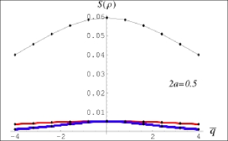
(a) $2a=0.5$

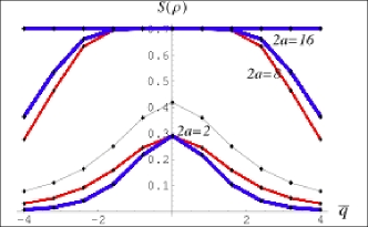
(b) Larger $2a$’s

Figure 5: (Color online) Comparison of the two different cases of preliminary measurements done by both parties together with the case that only one party makes a preliminary measurement. The entanglement $S(\hat{\rho}^{(A)})$ is plotted against the centre $\bar{q}$ of the preliminary-measurement region with width $2a$. (a) For $2a=0.5$. (b) For other larger values of $2a$. Red long-dashed line (Case 1): Both parties’ preliminary measurements localise their particles in regions with identical widths and centres ($a=b$ and $\bar{q}_{A}=\bar{q}_{B}$). Blue thick short-dashed line (Case 2): The widths of the regions are the same but one centre is always fixed around the centre of the wavefunction while there is no restriction on the other centre ($a=b$, $\bar{q}_{B}=0$). Black thin solid line (Case 3): Only one party makes a preliminary measurement. In all three cases, the number of bins used in the calculation is $N_{B}=100$ and $\alpha=6$.

Next we consider the case where both Alice and Bob make preliminary measurements, but not necessarily in the same way.

We start by considering two different cases; the first (Case 1) is that both parties’ preliminary measurements restrict their particles to regions with identical widths and centres ($a=b$ and $\bar{q}_{A}=\bar{q}_{B}$), whereas in the second case (Case 2) the region widths are the same but the centre of Bob’s region is always fixed around the centre of the wavefunction ($a=b$, $\bar{q}_{B}=0$). The results, for $\alpha=6$, are shown together with the previous result (Case 3; only Alice makes a preliminary measurement, as shown in Fig. 4(a)) for comparison in Fig. 5. The entanglement in the discarding ensemble of Case 3 is the highest out of the three cases; this is as expected, since the entanglement can only reduce under the additional (local) measurements made by Bob. When the width $2a$ is small, the entanglement of Case 1 is higher than of Case 2. However, as $2a$ increases, Case 2 converges more rapidly to Case 3 so that its entanglement is now higher than that of Case 1, until $2a$ becomes so large that the differences between all three cases disappear.

V.3.3 Both particles restricted: classical correlations

We now compare the entanglement distributions to the classical correlations between the particles. Suppose that Alice and Bob localise their respective particles to regions with the same widths but different centres; the entanglement in the discarding ensemble will depend on both $\bar{q}_{A}$ and $\bar{q}_{B}$. We shall compare the entanglement distribution with the 2-particle probability distribution $P(q_{A}\in\mathcal{A}\cap q_{B}\in\mathcal{B})$, and the conditional probability distribution for Bob’s particle given the position of Alice’s particle, $P(q_{B}\in\mathcal{B}\mid q_{A}\in\mathcal{A})$.

The two-particle probability is

$$P(q_{A}\in\mathcal{A}\cap q_{B}\in\mathcal{B}) = \int_{\bar{q}_{A}-a}^{\bar{q}_{A}+a}\mathrm{d}q_{A}\int_{\bar{q}_{B}-a}^{\bar{q}_{B}+a}\mathrm{d}q_{B}$$ (42)

$$\quad\rho(q_{A},q_{B};q_{A},q_{B}),$$

and in the limit of small $a,b$ we have

$$P(q_{A}\in\mathcal{A}\cap q_{B}\in\mathcal{B})=4ab\rho(\bar{q}_{A},\bar{q}_{B};\bar{q}_{A},\bar{q}_{B}).$$ (43)

The conditional probability is

$$P(q_{B}\in\mathcal{B}\mid q_{A}\in\mathcal{A})=\frac{P(q_{A}\in\mathcal{A}\cap q_{B}\in\mathcal{B})}{P(q_{A}\in\mathcal{A})},$$ (44)

where $P(q_{A}\in\mathcal{A})$ is the 1-particle probability. In the limit of small $a,b$ this becomes

$$P(q_{B}\in\mathcal{B}\mid q_{A}\in\mathcal{A})=2b\frac{\rho(\bar{q}_{A},\bar{q}_{B};\bar{q}_{A},\bar{q}_{B})}{\rho^{(A)}(\bar{q}_{A},\bar{q}_{A})}.$$ (45)

In each case the small-$a,b$ limit can be easily evaluated: we find

$$\rho(q_{A},q_{B};q_{A},q_{B})=\zeta_{2}\exp(-\frac{(\bar{q}_{A}+\bar{q}_{B})^{2}}{2\sigma_{+}^{2}}-\frac{(\bar{q}_{A}-\bar{q}_{B})^{2}}{2\sigma_{-}^{2}})$$ (46)

with ‘classical’ standard deviations

$$\sigma_{+}^{C} = \sqrt{2},$$

$$\sigma_{-}^{C} = (\frac{2}{\sqrt{1+4\alpha}})^{\frac{1}{2}},$$ (47)

and

$$\frac{\rho(\bar{q}_{A},\bar{q}_{B};\bar{q}_{A},\bar{q}_{B})}{\rho^{(A)}(\bar{q}_{A},\bar{q}_{A})}=\zeta_{3}\exp(-\frac{\bar{q}_{A}^{2}}{2\sigma_{1}^{2}}+\frac{\bar{q}_{A}\bar{q}_{B}}{2\sigma_{12}^{2}}-\frac{\bar{q}_{B}^{2}}{2\sigma_{2}^{2}})$$ (48)

with

$$\sigma_{1} = (\frac{(1+\sqrt{1+4\alpha})(1+2\alpha+\sqrt{1+4\alpha})}{4\alpha^{2}})^{\frac{1}{2}},$$ (49)

$$\sigma_{2} = (\frac{2}{1+\sqrt{1+4\alpha}})^{\frac{1}{2}},$$

$$\sigma_{12} = (\frac{1}{\sqrt{1+4\alpha}-1})^{\frac{1}{2}},$$

where $\zeta_{2}$ and $\zeta_{3}$ are normalization constants.

For finite $a$ and $b$ we capture the shape of the distributions by fitting the numerically calculated values of $P(q_{A}\in\mathcal{A}\cap q_{B}\in\mathcal{B})$, and $P(q_{B}\in\mathcal{B}\mid q_{A}\in\mathcal{A})$ using the same expressions Eq. (46) and Eq. (48), thereby extracting numerical values for $\sigma^{C}_{\pm}$, $\sigma_{1,2}$ and $\sigma_{12}$. We also use the function Eq. (46) to fit the entanglement distribution, thereby obtaining two further parameters $\sigma^{Q}_{\pm}$ which quantify the extent of the entanglement distribution along its principal axes.

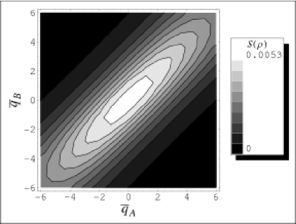
(a) $2a=0.5$

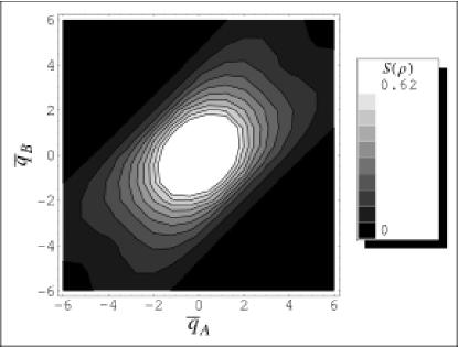
(b) $2a=4$

Figure 6: Dependence of the entanglement $S(\hat{\rho}^{(A)})$ on the locations of the centres of the preliminary-measurement regions $\bar{q}_{A}$ and $\bar{q}_{B}$. (a) the width $2a$ of the regions is 0.5. (b) $2a=4$. In both cases, $N_{B}=100$ and $\alpha=6$.

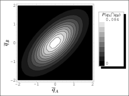
(a) $2a=0.5$

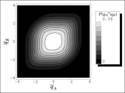
(b) $2a=4$

Figure 7: The dependence of the classical joint probability $P(q_{A}\in\mathcal{A}\cap q_{B}\in\mathcal{B})$ on $\bar{q}_{A}$ and $\bar{q}_{B}$. (a) $2a=0.5$. (b) $2a=4$. In both cases, $\alpha=6$.

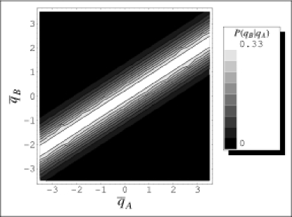
(a) $2a=0.5$

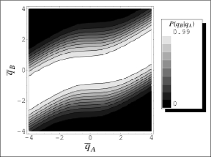
(b) $2a=4$

Figure 8: Dependence of the conditional probability $P(q_{B}\in\mathcal{B}\mid q_{A}\in\mathcal{A})$ on $\bar{q}_{A}$ and $\bar{q}_{B}$. (a) $2a=0.5$. (b) $2a=4$. In both cases, $\alpha=6$.

As before, we take $\alpha=6$. In Fig. 6, we show two cases of entanglement distributions for different widths ($2a=0.5$ and $2a=4$) of the preliminary-measurement regions. We see that the entanglement distribution with larger $2a$ is more symmetric. The corresponding joint probability distributions and conditional probability distributions are shown respectively in Fig. 7 and Fig. 8. (Note that the figures show different range of $\bar{q}_{A}$ and $\bar{q}_{B}$.) The classical probability distributions $P(\bar{q}_{A}\cap\bar{q}_{B})$ are more localized and symmetric in space than the entanglement distributions.

$\alpha=6$	$\sigma_{+}^{Q}$	$\sigma_{-}^{Q}$	$\sigma_{+}^{C}$	$\sigma_{-}^{C}$	$\sigma_{1}$	$\sigma_{2}$	$\sigma_{12}$
$2a\rightarrow 0$	$\infty$	$\infty$	1.41	0.632	0.866	0.577	0.500
$2a=0.5$	10.4	2.29	1.43	0.665	0.937	0.603	0.531
$2a=4$	3.44	2.10	2.37	2.00	11.0	1.53	2.64

Table 1: Table of $\sigma$ values for $\alpha=6$.

In the limit of very small $a$, $S(\hat{\rho}^{(A)})$ is constant everywhere (Eq. (40)) so $\sigma^{Q}_{+}$ and $\sigma^{Q}_{-}$ must diverge; the results in Table 1 show that $\sigma^{Q}_{+}$ diverges more quickly as $a$ reduces, while the two parameters become comparable for large $a$ as the entanglement distribution becomes more symmetric. Indeed, the distributions of the entanglement and the classical correlations become more alike as $2a$ increases, because both distributions are flat out to a distance $a$ either side of the wavefunction’s central peak.

We can also study the effect of varying the coupling strength $\alpha$ for a fixed (small) $2a$. We plot $\sigma_{+}^{Q}$ and $\sigma_{-}^{Q}$ against $\alpha$ with $2a=0.5$ in Fig. 9a whereas $\sigma_{+}^{C}$, $\sigma_{-}^{C}$, $\sigma_{1}$, $\sigma_{2}$ and $\sigma_{12}$ in Fig. 9b. The entanglement distribution is the most asymmetrical and as $\alpha$ increases, the difference between $\sigma_{+}^{Q}$ and $\sigma_{-}^{Q}$ widens. Of the quantities determining the classical probability distribution, $\sigma_{+}^{C}$ remains constant with increasing $\alpha$, but $\sigma_{-}^{C}$ gradually decreases. These trends arise because the two particles tend to move together when the spring joining them becomes strong. Therefore, as $\alpha$ increases, the white rod in Fig. 8 rotates about the centre of the square from the line $\bar{q}_{B}=0$ towards the diagonal $\bar{q}_{A}=\bar{q}_{B}$. $\sigma_{1}$ is always the largest out of the three parameters for the conditional probability distribution. For weak $\alpha$, $\sigma_{12}$ is larger than $\sigma_{2}$ but as $\alpha$ becomes larger, at some point the two plots intercept and $\sigma_{12}$ is no longer larger than $\sigma_{2}$.

How in the limit of very small $a$ these quantities (Eq. (47) and Eq. (49)) vary with $\alpha$ is shown in Fig. 9c. We see that the behaviour of these quantities do not change much, compared with the previous results when $2a=0.5$, apart from that the interception points happen at smaller $\alpha$. Note that $\sigma^{Q}_{\pm}$ diverge as $a\rightarrow 0$, so these parameters are not shown.

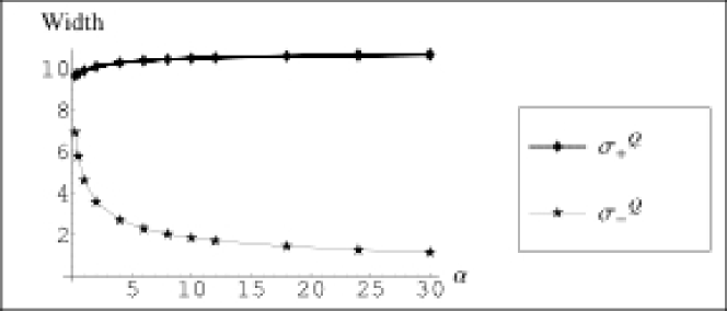
(a) $\sigma^{Q}_{\pm}$; $2a=0.5$

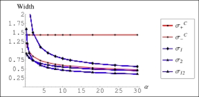
(b) $2a=0.5$

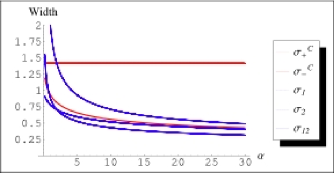
(c) Small-$a$ limit

Figure 9: (Color online) Plots of $\sigma_{+}$, $\sigma_{-}$, $\sigma_{1}$, $\sigma_{12}$ and $\sigma_{2}$ against $\alpha$. In the plot legend, $Q$ stands for the ‘quantum’ entanglement distribution and $C$ for the ‘classical’ probability distribution. (a) and (b): Numerical results: $2a$ is chosen to be 0.5 for all the cases. (c) Analytical results: in the limit of very small $a$.

VI Conclusions

We have presented a novel thought experiment that gives an approach to determining the location in configuration space of the entanglement between two systems. It involves choosing a region of the two-party configuration space and making a projective measurement with only enough resolution to determine whether or not the system resides in this region, then characterizing the entanglement remaining in the corresponding sub-ensemble. Our approach is particularly simple to implement for pure states, since in this case the sub-ensemble in which the system is definitely located in the required region after the measurement is also a pure state, and hence its entanglement can be simply characterized by the entropy of the reduced density operators.

We have given examples of the application of our method to states of a simple spin system, where Alice and Bob share two pairs of spin-1/2 particles, and also of a continuous-variable system in which they share a pair of coupled harmonic oscillators.

The first case shows how the amount of entanglement located in the chosen region (in this case the $M_{s}=0$ manifold) varies as the characteristics of the states shared by Alice and Bob are altered. We presented results for both pure and mixed states, and show how entanglement is affected by the “mixedness” $F$ both qualitativly and quantitativly. Specifically, we show that the states which are entangled from the global point of view are also entangled by our local measures Lin and Fisher (2006), i.e. global entanglement of the initial state vanishes at the same point as the entanglement remaining in the discarding ensemble after the preliminary measurement to locate the system in a chosen subspace.

For the second case we have presented results as a function of the strength of the coupling between the oscillators, as well as of the size and location of the preliminary measurement regions. In all cases the remaining entanglement saturates to the total entanglement of the system as the measured regions become large. For small measured regions the entanglement tends to zero, but for a fixed region size the configuration-space location can be varied in order to give a variable-resolution map of the entanglement distribution. We find that the distribution of the entanglement is qualitatively different from the classical correlations between the particles, being considerably more extended in configuration space than the joint probability density and becoming more and more diffuse as the size of the regions decreases.

Our approach suffers from the disadvantage that there is no sum rule on the entanglements in the discarding ensemble: the sum of the entanglements from all the sub-regions defined by a given decomposition of configuration space does not yield the full entanglement of the system. Instead, the entanglements from the sub-regions satisfy the inequality in Eq. (17). It would be interesting to understand in more detail the relationship between the restricted entanglements (as defined in this paper) and the full entanglement of the system, and also to extend the calculations reported here to projective measurements made in other bases, to POVMs, and to mixed states.