Quantum Optical Systems for the Implementation of Quantum Information Processing

Abstract

We review the field of Quantum Optical Information from elementary considerations through to quantum computation schemes. We illustrate our discussion with descriptions of experimental demonstrations of key communication and processing tasks from the last decade and also look forward to the key results likely in the next decade. We examine both discrete (single photon) type processing as well as those which employ continuous variable manipulations. The mathematical formalism is kept to the minimum needed to understand the key theoretical and experimental results.

I Introduction

Information is not independent of the physical laws that govern how it is stored and processed LAN91 . The unique properties of quantum mechanics imply radically different ways of communicating and processing information NIE00 . However, to realize the potential of quantum information science, quantum systems with very special properties are needed. For example, it is essential that the quantum system evolves coherently and thus must be well isolated from the surrounding environment, but, in order that the information stored in the system can be processed and read out, it must also be possible to produce very strong interactions between the system and classical meters and control elements. In this paper we will review progress in achieving quantum information processing in optics, where the system in question is the quantum state of an electro-magnetic field mode at optical frequencies.

I.1 Quantum Information

It was perhaps Wiesner WIE72 who first realized that there are information tasks that can be achieved more effectively using quantum systems as the information carriers when he introduced his quantum money in 1972. The idea was to provide security against counterfeiting by encoding part of the bank note’s serial number on quantum systems. This idea was famously extended to communications by Bennett and Brassard in 1984 BEN84 when they introduced quantum key distribution, a system for securely distributing a cryptographic key. Both of these applications depend on the unique property that quantum information can not be cloned WOO82 . That is, given a quantum system in an unknown state, it is not possible to produce an identical copy of the system (whilst retaining the original).

Other communication tasks that could be achieved only with quantum systems started appearing in the early 1990’s. A key realization was that entanglement could be used as a resource for such tasks. A pair of spatially separated quantum systems are said to entangled if the state that describes the joint system cannot be factored into a product of states describing the individual systems. For example if two distant parties share entanglement then they can communicate classical information at twice the classical rate through the technique of quantum dense coding BEN92 . Similarly, in the presence of entanglement, quantum information can be communicated via the exchange of classical information through the technique of quantum teleportation BEN93 .

Around the same time that Bennett and Brassard were first describing quantum communication, Feynman FEY86 noted the possibility that computer algorithms existed that could be more efficiently processed by quantum systems than classical systems. Although toy examples of such algorithms were suggested by Deutsch soon after DEU86 it was not till 1995 that Shor SHO94 showed that an important problem, the determination of prime factors, could be solved in exponentially less time using a processor based on quantum systems, a quantum computer. The key technique, quantum error correction, was developed soon after SHO95 ; STE96 . This enables coherent correction of the logical errors which will inevitably creep into any calculation on a quantum computer. Another influential algorithm, showing speed up for the searching of an unsorted data base, was subsequently developed by Grover GRO97 . These developments showed that fault tolerant quantum computers (i.e. where errors can be corrected in the presence of imperfect gate operations) were in principle possible and that such machines could solve interesting problems. This in turn led to an explosion of interest in the field of quantum information.

Quantum information was originally discussed in terms of binary systems. Consider a two-level quantum system. This could be the spin states of an electron: up or down; two well isolated energy levels of an atomic system or; many other possibilities including various optical field states as we shall describe later. It is clear that such two level systems could be used to carry bits of information. For example, we could assign the value “zero” to one of the states, writing it in Dirac notation SAK85 as $|\bf 0\rangle$, and “one” to the other state writing $|\bf 1\rangle$. A string of these objects could then faithfully represent an arbitrary bit string.

However, quantum objects offer more possible manipulations than classical carriers of bits. In particular not only can we have zero’s and one’s, but we can also have superpositions of zeros and ones such as the plus state $|+\rangle=(1/\sqrt{2})(|\bf 0\rangle+|\bf 1\rangle)$. Indeed bits can just as effectively be encoded in these superposition basis states, for example using $|+\rangle$ as a zero and $|-\rangle=(1/\sqrt{2})(|\bf 0\rangle-|\bf 1\rangle)$ as a one. Because of these extra degrees of freedom we refer to information digitally encoded on quantum systems as quantum bits or $\it qubits$ SCH95 .

One non-classical feature of encoding in this way is the fact that different bases do not in general commute. Thus simultaneous, ideal measurements in both bases cannot be made. Furthermore any measurements which obtain information about the bit values of one basis inevitably disturbs the bit values of the other basis. As we have mentioned these features (and more generally the no-cloning theorem) can be used to create a secure communication channel via the technique of quantum key distribution (also referred to as quantum cryptography).

Another feature of qubits is their ability to span all different bit values simultaneously. This is obviously true of a single qubit where the $|+\rangle$ state, when viewed in the computational basis, $|\bf 0\rangle$ and $|\bf 1\rangle$, equally spans the two different bit values, 0 and 1. This continues to be true for multi-qubit states. For example suppose we start with two qubits in the state

$$|\bf 0\rangle|\bf 0\rangle$$ (1)

where the first ket represents the first qubit and the second ket the second qubit and a tensor product is implied between their two Hilbert spaces. If we rotate both of them into their plus states we end up with the state

$$|\bf 0\rangle|\bf 0\rangle+|\bf 0\rangle|\bf 1\rangle+|\bf 1\rangle|\bf 0\rangle+|\bf 1\rangle|\bf 1\rangle$$ (2)

which is an equal superposition of all four possible two bit values. This generalizes to $n$ qubits where the same operation of rotating every individual qubit leads to an equal superposition of all $2^{n}$ bit values.

Although this ability to span all possible inputs simultaneously hints at the possibility of increased communication or computation power using qubits, it is not the whole story. Note in particular that analogues of the sort of superpositions represented by Eq. 2 can also be created in classical optical systems as superpositions of classical waves. In order to unlock the full power of quantum information we need to create entangled states such as the state

$$|\bf 0\rangle|\bf 0\rangle+|\bf 1\rangle|\bf 1\rangle$$ (3)

which clearly cannot be factored into contributions from the individual qubits and has no classical wave analogue.

If we consider information processing using qubits instead of classical bits we need to introduce quantum gates. Some of these will have classical counterparts, for example the NOT gate takes $|\bf 0\rangle$ to $|\bf 1\rangle$ and vice versa. On the other hand some gates will have no classical analogue, such as the Hadamard gate which takes $|\bf 0\rangle$ to $(1/\sqrt{2})(|\bf 0\rangle+|\bf 1\rangle)$ and $|\bf 1\rangle$ to $(1/\sqrt{2})(|\bf 0\rangle-|\bf 1\rangle)$. We also require two qubit gates such as the control-NOT (CNOT) which preforms the NOT operation on one qubit (the target) only if the other qubit (the control) has “one” as its logical value. Eventually, if large arrays of gate operations can be implemented efficiently, and fault tolerantly, on many qubits, one could consider performing quantum computation. Although considerable progress has been made, the realization of quantum computation experimentally still remains a long way off.

In more recent years quantum information research has been extended to systems with Hilbert space dimensions greater than two. In particular, there has been considerable interest in infinite dimensional Hilbert spaces and the quantum information properties of continuous degrees of freedom such as position and momentum BRA03 . Continuous variable versions of teleportation BRA98 and key distribution RAL00 ; HIL00 were developed early on and many other protocols followed. Quantum computation proposals based on continuous variables have also been developed GOT01 ; RAL03 .

I.2 Quantum Optics

The invention of the laser in the early sixties and its subsequent development led to an unprecedented increase in the precision with which light could be produced and controlled, and hence enabled the ability to systematically investigate the quantum properties of optical fields; quantum optics. The fundamental theoretical description of the quantized electromagnetic field was due to Dirac in the early days of quantum mechanics DIR58 . Stimulated by the new technological possibilities, Glauber GLA62 , Louiselle LOU73 and others laid the theoretical basis for the description of the laser and identified the signatures of non-classical light.

It was soon realized that quantum optics offered a unique opportunity to test fundamentals of quantum theory not previously available for experiments. The first experiments to demonstrate in a semi-controlled way the production of single light quanta or photons were arguably those of Kimble et al KIM77 based on the resonance fluorecense of single emitters, as proposed by Carmichael and Walls CAR76 . Pairs of photons produced by atomic cascades were shown to be in entangled states by Aspect, Grangier and Rogers ASP81 with non-classical correlations sufficiently strong to exclude all local-realistic hidden variable theories through violation of Bell inequalities BEL71 . These results followed from the earlier work of Clauser, et al CLA69 and Freedman FRE72 that adapted the original inequalities to the experimental setting. It should be noted that even now experimental efficiencies are not high enough to avoid the need for a fair sampling assumption in the data analysis of these types of experiments, thus not closing all ”loopholes” for these inequalities. Heralding of single photon states using atomic cascades GRA86 and parametric down conversion GHO87 followed. The latter technique uses a second order non-linearity to produce pairs of photons at half the pump frequency spontaneously, and has been the workhorse of photon experiments for the last twenty years. That the pairs of photons from down conversion can be made indistinguishable and hence exhibit Bosonic interference effects was shown in key experiments by Hong, Ou and Mandel HON87 .

Squeezed states, that exhibit non-classical statistics for their quadrature amplitudes, which are continuous variables, were discussed in the seventies YUE76 and eighties WAL83 and eventually demonstrated by Wu et al WU87 . Demonstration of entanglement between quadrature amplitudes, strong enough to demonstrate the paradox of Einstein, Podolsky and Rosen EIN35 , followed by Ou et al in the early nineties OU92 .

Light can be described quantum mechanically in terms of the mode annihilation operator ${\hat{a}}$, its conjugate, the creation operator ${\hat{a}}^{\dagger}$ and the electromagnetic field mode ground, or vacuum state $|0\rangle$. The action of the creation operator on the vacuum state is to create a single photon number state, in a single spatio-temporal mode, i.e. ${\hat{a}}^{\dagger}|0\rangle=|1\rangle$. In general ${\hat{a}}^{\dagger}|n\rangle=\sqrt{n+1}|n+1\rangle$ where $n$ is a positive integer. Similarly the annihilation operator annihilates a single photon in a particular single spatio-temporal mode and in general ${\hat{a}}^{\dagger}|n\rangle=\sqrt{n}|n-1\rangle$. The number states form an ortho-normal basis convenient for representing arbitrary states. The mode operators obey the commutation relation $[{\hat{a}},{\hat{a}}^{\dagger}]=1$. It is often convenient to pick our mode decomposition in terms of single frequency eigenstates using the nomenclature ${\hat{a}}_{\omega}$ and $|0\rangle_{\omega}$. Then we have

$$[{\hat{a}}_{\omega^{\prime}},{\hat{a}}_{\omega}^{\dagger}]=\langle 0|_{\omega^{\prime}}|0\rangle_{\omega}=\delta(\omega^{\prime}-\omega)$$ (4)

The optical observables of interest are the photon number, ${\hat{n}}={\hat{a}}^{\dagger}{\hat{a}}$, and the quadrature amplitude, ${\hat{X}}^{\theta}=e^{i\theta}{\hat{a}}+e^{-i\theta}{\hat{a}}^{\dagger}$. Photon number is proportional to intensity for bright fields and can be measured by photo-detectors. For dim fields individual photons can be resolved with photon counters. The quadrature amplitude of the field can be measured by beating the signal field with a bright, phase reference field at the same optical frequency, a local oscillator (LO), and then measuring it with by photo-detection. This is known as homodyne detection. The angle $\theta$ is the phase difference between the signal and the LO and is usually taken to be in-phase ($\theta=0$) or out-of-phase ($\theta=\pi$), giving two conjugate (i.e. non-commuting) variables analogous to position and momentum.

As well as the number states, another key state in quantum optics is the coherent states. The coherent states are displaced vacuum states defined by

$$|\alpha\rangle={\hat{D}}(\alpha)|0\rangle$$ (5)

where the displacement operator is

$${\hat{D}}(\alpha)=e^{i({\hat{a}}\alpha+{\hat{a}}^{\dagger}\alpha^{\ast})}$$ (6)

The coherent states are eigenstates of ${\hat{a}}$ with eigenvalue $\alpha$. This leads to average values for their quadrature observables that are the same as for a classical field with the same amplitude. Hence the coherent state is often thought of as the quantum mechanical state which is the closest approximation to a classical optical field. The output of a well stabilized laser is a mixed state which can be approximately decomposed as an ensemble of coherent states with fixed magnitude but random phases MOL97 . However, in situations where the phase is unimportant, or when the LO is derived from the same laser as the signal such that the phase is common mode, it is convenient to model laser output as being in a single coherent state of fixed magnitude and phase.

Because of the success in demonstrating fundamental quantum effects in optics, light was an obvious candidate for demonstrating the predictions of quantum information science. Here we will review quantum optics successes in quantum information science and look at its potential for achieving more complex quantum processing tasks in the future.

II Encoding Classical Information on Light

Before considering the quantum information potential of optics we first discuss the encoding of classical information on quantum states of light. Current optical communications systems operate in a regime in which quantum effects can be ignored. In the future, as higher and higher communication efficiency is required, this is likely to change. Here we consider the ultimate limits imposed by quantum mechanics. We quantify this using the channel capacity, a concept that describes the maximum amount of information that can be transmitted based on statistical arguments. More detailed reviews of the techniques for the encoding, propagating and decoding of information on quantum systems can be found in Ref. YAM86 and Ref. CAV94 .

The Shannon capacity SHA48 of a communication channel operating at the bandwidth limit is

$$C={{1}\over{2}}\log_{2}[1+{{S}\over{N}}]$$ (7)

where $N$ is the noise power (variance), assumed Gaussian, and $S$ is the signal power, also assumed Gaussian distributed. Here $C$ is in units of bits per symbol. Eq.7 can be used to calculate the channel capacities of quantum states with Gaussian probability distributions such as coherent states and squeezed states. Consider first a signal composed of a Gaussian distribution of coherent state amplitudes all displaced at the same quadrature angle, say $\theta=0$ ($\alpha$ real). The signal power $V_{s}$ is given by the variance of the distribution. The noise is given by the intrinsic quantum noise of the coherent states, $V_{n}=\langle{\hat{X}}^{2}\rangle-\langle{\hat{X}}\rangle^{2}=1$. Because the quadrature angle of the signal is known, homodyne detection can in principle detect the the signal without further penalty, thus the measured signal to noise is $S/N=V_{s}/V_{n}=V_{s}$.

In general the average photon number per bandwidth per second of a light beam is given by

$$\bar{n}={{1}\over{4}}(V^{+}+V^{-})-{{1}\over{2}}$$ (8)

where $V^{+}$ ($V^{-}$) are the variances of the maximum (minimum) quadrature projections of the noise ellipse of the state. These projections are orthogonal quadratures, such as in-phase and out-of-phase, and obey the uncertainty principle $V^{+}V^{-}\geq 1$. In the above example one quadrature is made up of signal plus quantum noise such that $V^{+}=V_{s}+1$ whilst the orthogonal quadrature is just quantum noise so $V^{-}=1$. Hence $\bar{n}=1/4V_{s}$ and so the channel capacity of coherent states with single quadrature encoding and homodyne detection is

$$C_{c}=\log_{2}[\sqrt{1+4\bar{n}}]$$ (9)

Showing in an experiment that a particular optical mode has this capacity would involve: (i) measuring the quadrature amplitude variances of the beam, $V^{+}$ and $V^{-}$, (ii) calibrating the sender’s signal variance and (iii) measuring the receiver’s signal to noise. If these measurments agreed with the theoretical conditions above then Shannons theorem tells us that an encoding scheme exists which could realize the channel capacity of Eq.9. An example of such an encoding is given in CER01 .

If the average photon number per symbol is such that $\bar{n}>2$, improved channel capacity can be obtained by encoding symmetrically on orthogonal quadratures and detecting both quadratures simultaneously using a 50:50 beamsplitter followed by dual homodyne detectors, one for each quadrature (equivalently heterodyne detection can be used). Because of the non-commutation of orthogonal quaratures there is a penalty for their simultaneous detection which reduces the signal to noise of each quadrature to $S/N=1/2V_{s}$. Also because there is signal on both quadratures the average photon number of the beam is now $\bar{n}=1/2V_{s}$. On the other hand the total channel capacity will now be the sum of the two independent channels carried by the two quadratures. Thus the channel capacity for a coherent state with dual quadrature encoding and heterodyne detection is

$$C_{ch} = {{1}\over{2}}\log_{2}[1+{{S}\over{N}}^{+}]+{{1}\over{2}}\log_{2}[1+{{S}\over{N}}^{-}]$$ (10)

$$= \log_{2}[1+\bar{n}]$$

which exceeds that of the single quadrature homodyne technique (Eq.9) for $\bar{n}>2$.

If we restrict ourselves to a semi-classical treatment of light the above channel capacities are the best achievable. However the channel capacity of the homodyne technique can be improved by the use of non-classical, squeezed light YUE78 . With squeezed light the noise variance of the encoded quadrature can be reduced such that $V_{ne}<1$, whilst the noise of the unencoded quadrature is increased such that $V_{nu}\geq 1/V_{ne}$. As a result the signal to noise is improved to $S/N=V_{s}/V_{ne}$ whilst the photon number is now given by Eq.8 but with $V^{+}=V_{s}+V_{ne}$ and $V^{-}=1/V_{ne}$, where a pure (i.e. minimum uncertainty) squeezed state has been assumed. Maximizing the signal to noise for fixed $\bar{n}$ leads to $S/N=4(\bar{n}+\bar{n}^{2})$ for a squeezed quadrature variance of $V_{ne,opt}=1/(1+2\bar{n})$. Hence the channel capacity for a squeezed beam with homodyne detection is

$$C_{sh}=\log_{2}[1+2\bar{n}]$$ (11)

which exceeds both coherent homodyne and heterodyne for all values of $\bar{n}$.

In principle, a final improvement in channel capacity can be obtained by allowing non-Gaussian states. The absolute maximum channel capacity for a single mode is given by the Holevo bound and can be realized by encoding in a maximum entropy ensemble of number states and using photon number detection. This ultimate channel capacity is

$$C_{Fock}=(1+\bar{n})\log_{2}[(1+\bar{n})]-\bar{n}\log_{2}[\bar{n}]$$ (12)

which is the maximal channel capacity at all values of $\bar{n}$.

III Optical Qubits

We now consider how quantum information can be carried by light. There are a number of ways in which qubits can be encoded optically which fall into two broad classes: dual rail and single rail encoding. In dual rail encodings two orthogonal quantum optical modes are used. In single rail encoding only one quantum optical mode is used, although a second classical mode is implicitly needed as a phase reference. In the following we will begin by describing these encoding techniques and discussing a number of examples. We will then focus on dual-rail encoding and discuss current experimental approaches and future prospects for ”better” qubits.

III.1 Dual Rail Encoding

Consider two orthogonal optical modes represented by the annihilation operators ${\hat{a}}$ and ${\hat{b}}$ and the vacuum modes $|0\rangle_{a}$ and $|0\rangle_{b}$. For brevity we will write $|0\rangle_{a}\otimes|0\rangle_{b}\equiv|00\rangle$. We define our logical qubits as $|{\bf 0}\rangle={\hat{a}}^{\dagger}|00\rangle=|10\rangle$ and $|{\bf 1}\rangle={\hat{b}}^{\dagger}|00\rangle=|01\rangle$. That is single photon occupation of one mode represents a logical zero, whilst single photon occupation of the other represents a logical one. This is dual rail encoding.

For example suppose $|0\rangle_{a}$ and $|0\rangle_{b}$ are spatio-temporal modes with identical profiles, polarization and centre frequency, synchronized in time, but spatially separated. Arbitrary single qubit operations can be achieved using a beamsplitter and two phase shifters as illustrated in Fig. 1. A beamsplitter is a partially reflecting mirror that can coherently combine two optical modes in a set ratio. The interaction in the figure produces the following Heisenberg evolution of the mode operators:

$${\hat{a}} \to \sqrt{\eta}{\hat{a}}+e^{i\theta}\sqrt{1-\eta}{\hat{b}}$$

$${\hat{b}} \to e^{i\phi}(\sqrt{1-\eta}{\hat{a}}-e^{i\theta}\sqrt{1-\eta}{\hat{b}})$$ (13)

where $\eta$ is the intensity reflectivity of the beamsplitter. We have assumed the optical elements are lossless, a reasonable assumption for modern components. We have also assumed perfect mode matching between the two input modes to the beamsplitter, something rather more difficult to arrange in practice. Eq.13 implies the following qubit evolution BAC04 :

$$|10\rangle \to \sqrt{\eta}|10\rangle+e^{i\phi}\sqrt{1-\eta}|01\rangle$$

$$|01\rangle \to e^{i\theta}(\sqrt{1-\eta}|10\rangle-e^{i\phi}\sqrt{1-\eta}|01\rangle)$$ (14)

which corresponds to an arbitrary single qubit unitary.

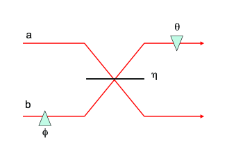
Figure 1: Beamsplitter and phase-shifter circuit for producing an arbitrary single qubit evolution on a spatial dual-rail qubit

More commonly two identical spatio-temporal modes but with different polarizations, say horizontal and vertical, will be used as the dual rails. Then we may write $|{\bf 0}\rangle=|10\rangle=|H\rangle$ and $|{\bf 1}\rangle=|01\rangle=|V\rangle$. Half and quarter-wave plates replace the phase shifters and beamsplitters in achieving arbitrary unitaries DOD03 . In particular the key operation the Hadamard gate, defined by $|{\bf 0}\rangle\to|{\bf 0}\rangle+|{\bf 1}\rangle$ and $|{\bf 1}\rangle\to|{\bf 0}\rangle-|{\bf 1}\rangle$, is implemented by a half wave-plate oriented at 22.5 degrees to the optic axis. Detection in any basis can be achieved via wave plates and polarizing beamsplitters which effectively converts polarization encoding into spatial encoding (see Fig. 2). The ease of manipulation and stabilty of polarization states has made this encoding the most popular in optics.

Another possibility is a temporal encoding in which the dual rails are spatio-temporal modes which are identical except for a time displacement STU02 . These can again be manipulated at the single qubit level with linear optics, though not deterministically unless fast electro-optic switches are available.

A final possibility is a frequency encoding in which, this time, the dual rail modes are identical except for a frequency off-set. Here an active element is required in order to move power coherently between different frequencies. If the frequency off-set is in the radio to micro-wave band then acousto-optic modulators and asymmetric interferometers can be used for this purpose HUN04 . Although the most difficult to manipulate the frequency encoding would likely be the most robust to fibre transmission.

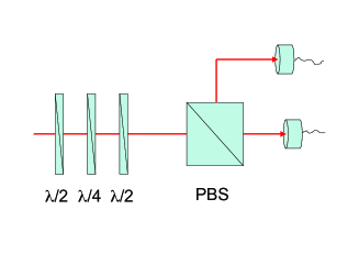
Figure 2: Combination of half and quarter wave plates oriented at particular angles, a polarizing beamsplitter (PBS) and photon counting, enables detection of polarization dual-rail qubits in any basis.

III.2 Single-Rail Encoding

Single-rail encoding requires only a single quantum mode, that can be placed into the states $|{\bf 0}\rangle=|\phi\rangle$ and $|{\bf 1}\rangle=|\psi\rangle$ or any superposition of them. The only requirement on these states is that they are orthogonal, i.e. that $\langle\phi|\psi\rangle=0$. In general such qubits will be non-stationary, so a good ”clock” is required in order to detect and manipulate them. In optics this clock, or phase reference, will typically be a classical optical mode derived from the master laser which is driving all the optical modes, in other words a local oscillator (LO).

Perhaps the simplest choice for $|\phi\rangle$ and $|\psi\rangle$ are the vacuum and single photon states, such that $|{\bf 0}\rangle=|0\rangle$ and $|{\bf 1}\rangle=|1\rangle$. Producing and manipulating superposition states of the form $\mu|0\rangle+\nu|1\rangle$, as required for this type of qubit is not so easy. However, a universal set of non-deterministic operations have been described LUN02 and superposition states have been produced non-deterministically in experiments LVO02 ; BAB04 . One important feature of the single-rail encoding is that it is relatively easy to produce entangled states. If a single photon is split on a 50:50 beamsplitter the resulting state is $(1/\sqrt{2})(|0\rangle|1\rangle+|1\rangle|0\rangle)$ which is a maximally entangled two qubit state in the single-rail encoding. Such states can then be used as a resource for quantum processing tasks.

Another possible choice for $|\phi\rangle$ and $|\psi\rangle$ are two different coherent states, such that $|{\bf 0}\rangle=|\alpha\rangle$ and $|{\bf 1}\rangle=|\beta\rangle$. In general such states will not be orthogonal but their overlap is given by $|\langle\alpha|\beta\rangle|^{2}=\exp[-|\alpha-\beta|^{2}]$ which is very small for quite modest differences in the amplitudes of the coherent states. A popular choice is to take $\beta=-\alpha$. By choosing $\alpha\geq 2$ a negligible overlap is achieved. The computational states, $|\alpha\rangle$ and $|-\alpha\rangle$ can be distinguished via homodyne detection. A useful feature of this choice is that the equal superposition state $|\alpha\rangle+|-\alpha\rangle$ ($|\alpha\rangle-|-\alpha\rangle$) contains only even (odd) photon number terms and so these orthogonal diagonal states can be distinguished by photon counting. A number of groups have discussed quantum information tasks using this encoding COC98 ; ENK02 ; JEO02 ; RAL03 . As for the single photon single-rail scheme, single qubit unitaries are difficult with this encoding but entanglement production is relatively easy. Indeed, splitting a superposition state like $|\alpha\rangle+|-\alpha\rangle$ many times on a beamsplitter leads to multi-mode entanglement. Whilst production of the coherent computational states is straightforward, to date the only experimental realizations of the superposition states have come from cavity quantum electro-dynamics experiments BRU96 ; TUR95 , though promising schemes LUN04 and initial results WEG04 suggest small traveling wave superposition states may be possible in the near future.

More exotic optical states have also been suggested for single rail encoding GOT01 that have nice error correction properties, but these are likely to be more difficult again to produce experimentally.

III.3 Postselection and Coincidence Counting

Producing and detecting single photon states efficiently is a major technological challenge. Currently the best single photon detectors have efficiencies around 90% and the most efficient single photon sources are around 55%, but typically in practical situations these numbers are much lower. This presents a major problem for single rail schemes where typically the loss of a photon results in a change to the qubit state and hence logical errors. In dual-rail schemes on the other hand, photon loss results in no qubit arriving (rather than the wrong qubit) and so can quite easily be filtered out of the data as we shall now describe. This is another reason why most optical quantum information demonstrations are currently based on dual-rail logic.

We begin by discussing how single photon experiments can be performed by strongly attenuating a single mode laser source. We can represent the state of such a laser source by the state

$$|\psi\rangle=|0\rangle+\alpha|1\rangle+{{\alpha^{2}}\over{2!}}|2\rangle+\ldots$$ (15)

As we attenuate the source more and more, $\alpha$ becomes much less than one and we can write to a good approximation

$$|\psi\rangle=|0\rangle+\alpha|1\rangle$$ (16)

We now have a source which in any particular time interval (length determined by the frequency dependence) has a high probability of producing vacuum; some small probability of producing a single photon state and; a negligible probability of producing a multi-photon state. If a photon counter is placed at the end of the experiment and we only worry about those times when the detector “clicks” then we will postselect just the single photon part of the state. If the source is polarized then it can be manipulated as a dual-rail qubit. Notice, however, that it is a rather inconvenient qubit source as it rarely works and you only know it worked after the fact, by evaluating the detection record. Never-the-less this type of source has successfully been used to demonstrate single qubit type experiments such as quantum key distribution (see section IV).

A major problem arises with an attenuated coherent source if we try to move to experiments requiring two qubits. One might assume we could use two highly attenuated coherent sources and then postselect only those events where two photons appear at the end of the experiment. However, the joint state of two equal power, attenuated lasers is

$$|\psi\rangle_{ab} = (|0\rangle+\alpha|1\rangle+{{\alpha^{2}}\over{2!}}|2\rangle+\ldots)_{a}$$ (17)

$$\;\;\;\;\;(|0\rangle+\alpha|1\rangle+{{\alpha^{2}}\over{2!}}|2\rangle+\ldots)_{b}$$

$$= |0\rangle_{a}|0\rangle_{b}+\alpha(|1\rangle_{a}|0\rangle_{b}+|0\rangle_{a}|1\rangle_{b})+$$

$$\;\;\;{{\alpha^{2}}\over{2!}}(2!|1\rangle_{a}|1\rangle_{b}+|2\rangle_{a}|0\rangle_{b}+|0\rangle_{a}|2\rangle_{b})+\ldots$$

where the first ket refers to one source whilst the second one to the other source. Notice that if we go to order $\alpha^{2}$ then there is indeed a term with a single photon state in each beam. However, terms involving pairs of photons in one beam with vacuum in the other occur with the same probability. Postselecting on two photon events will not in general remove these terms. Hence it is not possible in general to perform two qubit experiments using highly attenuated laser sources. A more sophisticated solution is required.

Since the late eighties, the solution of choice has been parametric down conversion in a $\chi_{2}$ medium GHO87 . Weak parametric down conversion results in the spontaneous converstion of single pump photons at the harmonic frequency into pairs of photons at the fundamental. If the down conversion is spatially non-degenerate then, in the Schrödinger picture, initial vacuum inputs are transformed according to

$$|0\rangle_{a}|0\rangle_{b}\to(|0\rangle_{a}|0\rangle_{b}+\chi^{\prime}|1\rangle_{a}|1\rangle_{b}+\chi^{\prime 2}|2\rangle_{a}|2\rangle_{b}+\ldots)$$ (18)

where $\chi^{\prime}$ is an effective non-linear interaction strength, proportional to the pump power. If we now allow $\chi^{\prime}$ to be very small, which is not hard to arrange experimentally, then the state produced is given to an excellent approximation by

$$|\psi\rangle_{ab}=|0\rangle_{a}|0\rangle_{b}+\chi^{\prime}|1\rangle_{a}|1\rangle_{b}$$ (19)

In contrast to equ.(17) the state in equ.(19) has only the desired two photon term to first order in $\chi^{\prime}$. If we postselect only those events from the detection record in which 2 photons are detected “simultaneously” or in coincidence (within some preset time window) then we will only record the part of the state which is due to the pairs of photons. Thus by using the combination of parametric down-conversion, the polarization degree of freedom and postselection, we can perfom, at least in principle, 2 qubit experiments. Experiments carried out this way are sometimes referred to as coincidence basis experiments and we will discuss various examples in later sections. However, note that this source is still spontaneous, ie successful events are rare, random and we do not know if they have occurred until after the fact. Although, 3 and 4 qubit experiments have been achieved by a simple generalization of the techniques just outlined, the cost is an exponential drop in the probability of success. Thus, although experiments carried out in coincidence can demonstrate the basic physics of particular systems, they are intrinsically not scaleable to large scale quantum information processing. Progress in producing sources without this drawback are discussed in the next section.

III.4 True Single Photon Sources

We now discuss two distinct approaches to producing better approximations to single photon states. The first is to create a heralded single photon source. That is a source which, though not always producing a single photon state, produces a clear signal when successful. Such a source could be made semi-deterministic by the use of quantum memory. The second approach is to produce an on-demand source, which deterministically produces a single photon state when requested.

III.4.1 Heralded Single Photons

By detecting one of the output modes and only accepting the other output if a photon is detected, a heralded single photon source can be created using spatially non-degenerate down-conversion. From an idealistic point of view the conditional state when a single photon is detected in mode $a$ can be obtained from equation (19) as

$$\langle 1|_{a}|\psi\rangle_{ab}=\chi^{\prime}|1\rangle_{b}$$ (20)

indicating that a single photon state is created in mode $b$ with probability $|\chi^{\prime}|^{2}$. In reality things are not so simple.

We expand the output state of the down-converter in a basis of wave-number eigenstates, each defining a single frequency spatial mode, to obtain

$$|\psi\rangle_{ab}=|0\rangle_{a}|0\rangle_{b}+\chi^{\prime}\int dk_{a}dk_{b}F(k_{a},k_{b})|1\rangle_{a}|1\rangle_{b}$$ (21)

where $k_{i}$ is the wave vector of the $i$th beam and the function $F(k_{a},k_{b})$ describes the spatio-temporal structure of the modes. The intrinsic spatio-temporal resolution of the photon counter far exceeds the read-out resolution. Thus the photon counter selects an ensemble of distinguishable single photon modes of which the experimenter is ignorant. This situation can be described by the mixed state

$$\rho_{a}=\int dk_{a}T(k_{a})|1\rangle_{a}\langle 1|_{a}$$ (22)

where $T(k_{a})$ is the spatio-temporal distribution of the detected ensemble. The output state, conditional on a photon count, is then

$$\rho_{b}=Tr_{a}[|\psi\rangle_{ab}\langle\psi|_{ab}\rho_{a}]$$ (23)

In general $\rho_{b}$ is a mixed state, however if $T(k_{a})$ is centred on but much “narrower” (both spatially and temporally) than $F(k_{a},k_{b})$, then to a good approximation the pure single photon number state

$$|\psi\rangle_{b}=\chi^{\prime}\int dk_{b}T(k_{b})|1\rangle_{b}$$ (24)

is produced.

Perhaps the most conclusive demonstration of photon production by this (or indeed by any) method was the experiment by Lvovsky et al.LVO01 . A beta-barium borate crystal was used in a type I arrangement to produce frequency degenerate but spatially non-degenerate photon pairs. Transform limited pulses at 790[nm] from a Ti:Sapphire laser were doubled and used to pump the crystal. Dispersion tends to make the pump and signal beams follow different paths through the crystal. Great care was taken to minimize any distortions of the spatial and temporal modes of the outputs due to this walk-off of the pump beam. The trigger photons were passed through a spatial filter and a $0.3$ [nm] frequency filter before being counted on a single photon detector. The success of the heralding process was characterised by performing homodyne tomography on the conditionally produced photon states. For best results the local oscillator pulse (LO) used in the homodyne detection of the signal must be accurately mode-matched to the single photon state. Mode matching with a visibility of about $80$% was achieved.

The homodyne data collected was then used to produce the Wigner distribution of the single photon state SMI93 . The Wigner distribution is a quasi-probability function for the quadrature amplitudes of the field state. The marginal distributions for the individual quadratures obtained from the Wigner function correspond to their respective probability distributions. Normalization of the distribution was achieved by simultaneously collecting vacuum state data. The resulting Wigner function was consistent with a mixed state comprised of $55$% single photon state and $45$% vacuum. Although imperfect the single photon state was still pure enough to display negative regions in the Wigner distribution, a highly non-classical effect that demonstrates the strongly quantum mechanical nature of the detected single photon state.

Lvovsky et al’s results clearly show that a single photon state can in principle be produced in this manner but it also highlights problems with this approach. For example, in order to obtain a conditional state which is as pure as possible, strong attenuation was applied to the trigger photon resulting in low single photon state production rates of about one photon every 4 seconds. Also, mode matching of the single photon state is seen to be a difficult problem. A more promising and practical solution would be to mode-match the single photon state into an optical fibre for subsequent use down-stream. The best results to date for this difficult problem were achieved by Kurtsiefer, Oberparleiter, and Weinfurter KUR01 who obtained about $40$% single photon contribution to the conditional state,

Finally, it is clearly inconvenient that the photons in these experiments are produced at random times. A possible solution to this problem suggested by Migdall, Branning and Casteletto MIG02 is to pump many crystals simultaneously so that the probability that at least one of them produces a pair is high. Electro-optic switches could then route the successfully triggered photon into the output mode (see Fig. 3(a)). Another solution to this problem, proposed and demonstrated in principle by Pittman, Jacobs, and Franson PIT02 , is to inject the single photon state into an optical fibre storage loop when the trigger photon is detected. The captured photon is then held there till required, when it is switched out of the loop (see Fig. 3(b)). If the round trip time of the loop is matched to the repetition rate of the pulsed pump laser then a number of loops can be loaded and then released simultaneously to produce several single photons states at the same time. Currently (as well as the mode matching problem discussed above) the losses associated with the Pockell cells used to switch the photons are prohibitively large.

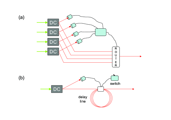
Figure 3: Two schemes for producing pseudo on-demand sources from heralded sources. In (a) an array of downconverters (DC) are pumped simultaneously. Photon counters monitor one of the output modes of each DC to see if it fired. If one of the counters triggers the other mode of the corresponding DC is sent to the output via an optical router. For a sufficiently large array the probability of at least one DC producing a pair becomes large. In (b) a single DC is pumped. If the trigger detector fires a fast optical switch captures the photon in a delay line. At some later time the photon can be released on demand by flicking the optical switch open.

III.4.2 Single Photons on Demand

The dream of a push-button single photon source can most nearly be realized by generating light from a single isolated emitter such as a single ion or atom. The trick here is that a single emitter can only produce a single photon “at a time” with some dead time between emissions while the source is re-excited. The effect is that the output state can be written (in an idealised fashion) as

$$|\psi\rangle=|0\rangle+\alpha|1\rangle+\tau({{\alpha^{2}}\over{2!}}|2\rangle+\ldots)$$ (25)

where $\tau$ is a number between $0$ and $1$ representing the suppression of higher photon number terms. If $\tau$ is very small then $\alpha$ can be made large, such that there is a high probability that a single photon will be emitted, whilst the probability of multiple photon emission remains very low.

The first experiments of this kind were performed in the late seventies KIM77 . However, although they clearly displayed the photon anti-bunching expected of a single photon source, they were very inefficient because they radiated into $4\pi$ steradians and, being based on atomic beams, there was little that could be done to improve matters. More recently various attempts have been made to create more efficient single emitters. These included: placing single neutral atoms or ions into high finesse optical cavities KUH02 ; KEL04 such that the photon emission should be into a single Gaussian mode; close coupling to single solid-state emitters such as neutral vacancy (NV) centre in diamond BEV02 and; the construction of single quantum-dot emitters integrated into distributed Bragg reflector (DBR) cavities SAN02 .

Initial experiments on quantum dot emitters were carried out by Santorini et al. SAN02 . Self-assembled InAs quantum dots embedded in GaAs were sandwiched between DBR mirrors to form tiny, high finesse, monolithic cavities in the form of $5$ micron high pillars. These were then cooled to 3-7 [K] and pumped by a pulsed Ti:Sapphire laser. The quantum dot emission, at around 935[nm], was spectrally filtered (0.1 [nm]) and a single polarization was selected before being coupled into single-mode optical fibre. The efficiency of single photon production was estimated to be about $30$%.

The single-photon states thus produced were characterized by their $g^{(2)}$ factor which was typically of the order of $0.06$ ($\tau^{2}\approx g^{(2)}$) showing good suppression of two photon emission. To test the indistinguishability of the photon states the Hong-Ou-Mandel dip HON87 between consecutive emissions was measured. The inferred visibility of the dip when measurement imperfections were taken into account was about $70$%.

Intrinsic time-jitter due to the spontaneous excitation process employed has been identified as the prime cause of the loss of photon indistinguishability between pulses in the quantum dots KIR03 . The prospects for indistinguishability between independent emitters are more remote due to the inherent variability of the structures. A different approach which does not suffer from these drawbacks is to place a single ion in a high finesse cavity, as demonstrated by Keller et al KEL04 . A single calcium $40$ ion was trapped inside an 8mm, high finesse cavity with a $1.2$ MHz decay rate. After laser cooling, a photon is produced through a cavity assisted Raman process, which is coherent and does not suffer from inhomogeneous broadening. Suppression of two photon events was $\tau^{2}\approx 0.01$ and detection limited. The device could produce a stream of single photon events over more than an hour, at a repetition rate of $100$ KHz and a photon production efficiency of about $5$%. Photon temporal indistinguishability was confirmed through observation of the photon wave-packet spread via the photon arrival time probability distribution.

The advantages in purity of the ion-trap photon source over the quantum dots comes at the price of a much more complicated set-up and much slower repetition rates. For both systems, the modest efficiencies mean that they are still effectively spontaneous sources. However, progress is rapid and we may anticipate systems combining the best aspects of the present systems with high efficiency in the not too distant future.

III.5 Characterising photonic qubits and processes

We now discuss the characterization of photonic qubits and processes. Our analysis assumes postselection, i.e. we only consider events in which a photon is detected. Of course this characterization cannot be carried out for a single event because of the probabilistic interpretation of quantum mechanics. But given a large ensemble of detection events, corresponding to identically prepared photons and/or interactions, a recipe can be given for determining the state of the ensemble or the process through which the ensemble was evolved.

We consider polarization encoded qubits. The polarization state of the photons is most generally described by the density operator ${\hat{\rho}}$. Our observables are the Stokes operators (corresponding to the classical Stokes parameters STO52 )

$${\hat{S}}_{1} = {\hat{n}}_{H}-{\hat{n}}_{V}=|H\rangle\langle H|-|V\rangle\langle V|$$

$${\hat{S}}_{2} = {\hat{n}}_{D}-{\hat{n}}_{A}=|H\rangle\langle V|+|V\rangle\langle H|$$

$${\hat{S}}_{3} = {\hat{n}}_{R}-{\hat{n}}_{L}=i(|V\rangle\langle H|-|H\rangle\langle V|)$$ (26)

where ${\hat{n}}_{J}$ is the number operator for the $J$th polarization mode. The eigenstates of ${\hat{S}}_{1}$ are $|H\rangle$ and $|V\rangle$ with eigenvalues $+1$ and $-1$ respectively. Similarly the eigenstates of ${\hat{S}}_{2}$ are $|D\rangle$ and $|A\rangle$ and of ${\hat{S}}_{3}$ are $|R\rangle$ and $|L\rangle$. The expectation values of the Stokes operators are related to measurement by

$$\langle{\hat{S}}_{1}\rangle = {{2R_{H}}\over{R_{H}+R_{V}}}-1$$

$$\langle{\hat{S}}_{2}\rangle = {{2R_{D}}\over{R_{H}+R_{V}}}-1$$

$$\langle{\hat{S}}_{3}\rangle = {{2R_{R}}\over{R_{H}+R_{V}}}-1$$ (27)

where $R_{H}$ and $R_{V}$ are the count rates recorded at the $H$ and $V$ output ports respectively of a horizontal/vertical polarizing beamsplitter and similarly for the diagonal/anti-diagonal and right/left bases.

On the other hand we can also express the expectation values in terms of the density operator as

$$\langle{\hat{S}}_{1}\rangle = Tr[{\hat{\rho}}{\hat{S}}_{1}]=\rho_{h,h}-\rho_{v,v}$$

$$\langle{\hat{S}}_{2}\rangle = Tr[{\hat{\rho}}{\hat{S}}_{1}]=\rho_{h,v}+\rho_{v,h}$$

$$\langle{\hat{S}}_{3}\rangle = Tr[{\hat{\rho}}{\hat{S}}_{1}]=i(\rho_{h,v}-\rho_{v,h})$$ (28)

where $\rho_{i,j}=\langle I|{\hat{\rho}}|J\rangle$ are the elements of the density matrix $\rho$ representing the density operator in the $H/V$ basis. Equations (28) are obtained using the ket representation of the Stokes operators given in equation (26). Combining equations (27) and (28) we can obtain all the elements of the density matrix in terms of the Stokes operators expectation values and hence in terms of count rates. The density matrix contains all the information about the polarization state of the photons and properties such as the purity of the state are readily extracted. A question often asked is how similar the experimentally produced state, ${\hat{\rho}}$, is to some pure target state $|\phi\rangle$. A common measure of this is the fidelity, $F$, given by

$$F=\langle\phi|{\hat{\rho}}|\phi\rangle$$ (29)

which is easily found in terms of the matrix elements of $\rho$. This technique can be extended to two, or more, photons by considering the expectation values of products of Stokes operators of each photon. For example

$$\langle{\hat{S}}_{1,a}{\hat{S}}_{1,b}\rangle=\rho_{hh,hh}-\rho_{hv,hv}-\rho_{vh,vh}+\rho_{vv,vv}$$ (30)

where $a,b$ label the two photons and $\rho_{ij,kl}=\langle i|\langle j|{\hat{\rho}}|k\rangle|l\rangle$. By considering the expectation values of all the different combinations of Stokes operator products the two photon density matrix can be characterised. Whilst 4 measurements are needed to completely characterise a single photon, 16 measurements are needed in general for two photons. Of course if the two photons are known to be in a separable state then 4 measurements on each individual photon will suffice to characterise the state. The greater number of measurements needed to characterise entangled states points to their increased complexity. The exponential increase in measurements required as a function of photon number continues with three photons requiring 64 measurements and so on.

The above techniques were developed and applied by White and James et al WHI99 , JAM01 . One problem that arises is that, due to experimental errors, the density matrix produced from the data may be unphysical. To deal with this, maximum likelihood techniques were applied such that the “closest” physical density matrix to the data can be identified JAM01 .

An unknown process can also be characterized by tomographic techniques NIE00 . An arbitrary single qubit process takes an input state ${\hat{\rho}}$ to an output state ${\hat{\rho}}^{\prime}$. This can be written quite generally in terms of the Stokes operators as

$${\hat{\rho}}^{\prime}=\sum_{i,j=0,3}w_{ij}{\hat{S}}_{i}{\hat{\rho}}{\hat{S}}_{j}$$ (31)

where we have introduced the Stokes identity operator: ${\hat{S}}_{0}=|H\rangle\langle H|+|V\rangle\langle V|$. The coefficients, $w_{ij}$, form a matrix that completely describes the process. The process matrix can be determined from the expectation values of the Stokes operators evaluated for a complete set of input states. As a result 16 mesurement settings are required for single qubit process tomography. these techniques can be generalized to multi-qubit processes with a corresponding exponential increase in the number of measurements required. The process matrix corresponding to a CNOT gate is shown in Fig.4. An experimental demonstration of process tomography on a two qubit circuit has been implemented in optics by O’Brien and Pryde et al JOB04 .

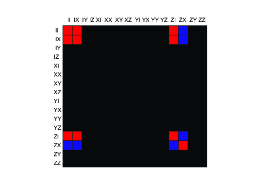
Figure 4: Process matrix in the Stokes (equivalently Pauli) basis of the two qubit entangling gate the CNOT. Red = +0.25; yellow = -.25; black = 0.

IV Quantum Key Distribution

Perhaps the most straightforward application of quantum information technology is in the field of secure communications. It is referred to variously as quantum key distribution (QKD), quantum cryptography or sometimes quantum key expansion and was initially proposed by Bennett and Brassard BEN84 . The idea is to set up a communication channel which is secure in the sense that any attempt to eavesdrop on the communication can be detected after the fact. The channel is used to send a random number encryption key between two parties, usually referred to as Alice (the sender) and Bob (the receiver). The parties then check if an eavesdropper, called Eve, intercepted any information about the key. If no Eve was present they can proceed to use the random number key to encrypt secret messages. If they find an Eve is present they scrap that key and try again.

Actually in any practical situation there will always be some errors in the transmission due to imperfections in the system. Thus what Alice and Bob do in practice is to set limits on the amount of information that Eve can have obtained based on the error rate they observe. Provided this error rate is sufficiently small, post processing of the data using techniques called error reconciliation and privacy amplification BEN95 can be used to produce a shorter secret key. Eve’s information about this shorter key can be made vanishingly small. Another important caveat is that Alice and Bob must initially share some secret information which they can use to identify each other. Otherwise Eve can fool them by pretending to be Bob to Alice and vice versa. Given these conditions QKD is provably secure GOT03 . No comparable result exists for classical communications.

IV.1 QKD using Single Photons

QKD’s ability to detect eavesdroppers is based on the fact that any process which acquires information about an observable of a quantum mechanical system inevitably disturbs the values of other non-commuting observables. To illustrate this consider the situation in which Alice is trying to communicate zero’s and one’s to Bob using polarized photons. First suppose Alice sends out a “zero” encoded as a horizontally polarized photon, $|H\rangle$. Eve measures in the horizontal/vertical basis and obtains the result “zero” and so sends a horizontally polarized photon on to Bob who will definitely get a zero if he measures in the horizontal/vertical basis. However, now suppose Alice and Bob switch to encoding in the diagonal/anti-diagonal basis without Eve knowing. Alice sends a zero as a diagonally polarized photon, $|D\rangle=(1/\sqrt{2})(|H\rangle+|V\rangle)$. Eve still measures in the horizontal/vertical basis and so has a 50/50 possibility of getting either zero or one as the result, regardless of what Alice sent. Further more, what Eve sends on to Bob is basically the mixed state $\rho=1/2(|H\rangle\langle H|+|V\rangle\langle V|)$. So when Bob measures in the diagonal/anti-diagonal basis he also gets a random result. Thus, by measuring in the wrong basis, not only does Eve potentially get the wrong result, but she also completely erases the qubit value which is sent on to Bob who then may also get the wrong result.

The trick then is to arrange a situation in which Eve does not know in which basis the information on any particular photonic qubit has been encoded because then she is bound to make mistakes which Bob will be able to detect. A typical protocol would go as follows:

1. Alice sends a random number sequence to Bob, encoded on the polarization of single photons. She randomly swaps between encoding on the horizontal/vertical basis and encoding on the diagonal/anti-diagonal basis.

2. Bob measures the polarization of the incoming photons and records the results, but he also swaps randomly between measuring in the horizontal/vertical basis and measuring in the diagonal/anti-diagonal basis.

3. After the transmission is complete Alice and Bob communicate on a public channel. First Bob announces which basis he measured for each transmission event. Alice tells him whether or not this corresponded to the basis in which she prepared the photon. They discard all transmission events for which their bases did not correspond.

4. Bob then reveals the bit values he measured for a randomly selected subset of the remaining data. Alice compares the values revealed by Bob with those she sent. Inevitably there will be some errors in the transmission. If this error rate is below a certain threshold then reconcilliation and privacy amplification can be employed to distill a secret key. If there are too many errors the data is discarded and they try again.

The first experimental demonstration of QKD was carried out by Bennett and co-workers in 1992 over a distance of centimetres BEN92a . Demonstrations over distances of tens of kilometers were first carried out by Hughes et al in free space HUG02 and by Gisin et al in fibre STU02 . Typically highly attenuated lasers are used as the qubit source. Switching between the four input states may be achieved through electro-optic control or via the passive combination of four separate laser sources. In all cases it is crucial that the spatial and temporal modes of the four input states are identical so that no additional information is leaked to Eve. The receiver station can be a passive arrangement. A 50/50 beamsplitter is used to randomly send the incoming photons either to a horizontal/vertical analyser or a diagonal/anti-diagonal analyser.

To increase the signal to noise of the detection system the detectors are gated, only opening for the one nanosecond or so window in which the single photon pulse is expected. Synchronization may be arranged via bright timing pulses preceding the single photon pulses or via more standard public communication links. Sophisticated reconciliation and privacy amplification algorithms then need to be implemented over the public channel.

The main motivation for free space systems is to transmit secret keys to satellites securely. For terrestrial systems transmission through fibre optic networks is more desirable. Although this has the advantage of less stray light, it has the problem that optic fibre is birefringent and hence polarization encoded qubits can become scrambled. One solution is to go to the temporal mode qubit encoding. For example one could use the non-commuting encodings

$$|\bf 0\rangle \equiv |T1\rangle+|T2\rangle$$

$$|\bf 1\rangle \equiv |T1\rangle-|T2\rangle$$ (32)

and

$$|\bf+\rangle \equiv |T1\rangle+i|T2\rangle$$

$$|\bf-\rangle \equiv |T1\rangle-i|T2\rangle$$ (33)

where $|Ti\rangle$ represents a single photon occupying a temporal wave packet centred at time $Ti$. Alice could produce the state $|T1\rangle+|T2\rangle$ by allowing a single photon pulse to pass through a Mach Zehnder interferometer with unequal arm lengths, in particular where the arm length difference is $T1-T2$. The other states are created in a similar way but where an additional phase of $\pi$ (for the state $|T1\rangle-|T2\rangle$) or $\pi/2$ or $3\pi/2$ (for the other basis states) is added to one arm of the interferometer. Unfortunately, a readout by Bob would require him to have an interferometer which is phase-locked to Alice’s , something that is difficult to arrange. An elegant solution to this problem is for Bob to first send a bright pulse to Alice STU02 . This pulse acts as a phase reference, thus avoiding the locking issue.

A limit on the secure key rates occurs with the use of attenuated laser sources. The initial intensity cannot be too great otherwise the probability of two-photon events will be too high. Eve can use two photon events to extract information about the key without penalty. One solution to this problem is to use a true single photon source (see section III.4). Beveratos et al. BEV02 were the first to demonstrate such a scheme. They used the fluorescence from a single NV colour centre inside a diamond nano-crystal at room temperature as their single photon source.

The QKD protocol we have discussed here is called BB84. Many other protocols have been proposed and demonstrated and new protocols and demonstrations appear regularly GIS02 . Initial steps to commercialization have already been taken.

IV.2 QKD using Continuous Variables

An alternative approach to QKD is to use non-commuting continuous variables such as the in-phase and out-of-phase quadratures. We saw in section II that information can be encoded on the quadrature amplitudes and read out using homodyne detection. We now examine the use of these techniques for QKD.

Recall the basic mechanism used in QKD schemes is the fact that the act of measurement (by Eve) inevitably disturbs the system. This measurement back-action of course also exists for continuous quantum mechanical variables. In particular let us consider the situation in which Alice sends a series of weak coherent states to Bob whose amplitudes are picked from a two-dimensional Gaussian distribution centred on zero. Bob chooses to measure either the in-phase or out-of-phase projections of the states onto a shared local oscillator using homodyne detection. Bob will effectively see a Gaussian distribution of real amplitude coherent states when he looks in-phase and a Gaussian distribution of imaginary amplitude coherent states when he looks out-of-phase. Alice can encode two different random number sequences on the two. Because the two quadrature measurements do not commute Eve now has a similar problem as in the discrete case: any attempt to extract information about one quadrature from the beam will inevitably erase information carried on the other quadrature. If Alice and Bob compare some of the data at the end of the protocol they will thus notice increased error rates as a result of any intervention. This protocol was developed by Grosshans and Grangier GRO02 based on earlier work RAL00 ; CER01 and has been developed considerably since SIL02 ; WEE04 ; GRO05 . Security proofs for coherent state protocols are based on various reasonable assumptions however, a proof of absolute security on par with those made in the discrete case has only been made for a somewhat different continuous variable protocol based on squeezed states GOT02 .

Coherent state QKD can be implemented either by sending very weak coherent pulses of light or by sending bright, quantum limited light with in-phase or out-of-phase amplitude modulation playing the role of the coherent states. The first in principle experimental demonstration of this technique was performed by Grosshans et al. GRO03 using the former technique. Recently the latter technique has been employed LOR04 ; LAN05 . In the experiment of Lance et al LAN05 end to end key exchange in the presence of 90% loss was achieved with a secret key rate of 1Kbit/s with a 17MHz bandwidth. Since this scheme is truly broadband, it can potentially deliver orders of magnitude higher key rates by extending the encoding bandwidth with higher-end telecommunication technology.

V Quantum Teleportation

We have seen that quantum communication can be more secure than classical communication. When entangled states are allowed a number of new enhanced communication and processing tasks become possible. This is quite remarkable given that entanglement is undirected and carries no information itself. For example, in the presence of entanglement, the classical capacity of a quantum channel (ie the ability of a quantum system to carry classical information) is increased. This is called quantum dense coding and has been described both in the discrete BEN92b and continuous domains BRA00 ; RH02 . In principle experimental demonstrations have also been made in both domains MAT96 ; PAN00 . Another example is quantum state sharing. Here an unknown quantum state can be distributed between $n$ parties in such a way that if $m$ of the parties collaborate (where $m<n$), then the state can be retrieved, but less than $m$ parties can not retrieve the state. Again both discrete CLE99 and continuous TYC03 protocols are known and an experimental demonstration has been made in the continuous case LAN04 .

Perhaps the most surprising (and most useful) of such tasks is quantum teleportation BEN93 . Here the presence of entanglement enables Alice to send Bob an unknown qubit by simply sending a classical message. To understand the novelty of this consider first what Alice can do in the absence of entanglement. Her best strategy is to measure the qubit in some basis and send a message that tells Bob to make a qubit corresponding to the result she gets. Sometimes she will be lucky and will measure in a good basis, then Bob will make a close approximation to the qubit. Other times she will measure in a bad basis and the result she gets will be completely random and Bob will make a poor approximation to the qubit. It can be shown that on average the fidelity of Bob’s qubit with Alice’s original is $2/3$.

If they share entanglement they can perform teleportation. This works in the following way: Alice and Bob share an entangled pair of qubits, say $|0\rangle_{a}|0\rangle_{b}+|1\rangle_{a}|1\rangle_{b}$ where the subscripts indicate the party that has the qubit. Alice also has a qubit in the arbitrary state $\mu|0\rangle_{a^{\prime}}+\nu|1\rangle_{a^{\prime}}$ which she wishes to send to Bob. Alice does not know the state of her qubit. If we write down the state of the three qubits and then rearrange it we notice a remarkable feature: Bob’s qubit can be represented as an equal superposition of four states, each differing from Alice’s unknown qubit by at most a bit-flip and a phase-flip.

$$(\mu|{\bf 0}\rangle_{a^{\prime}} + \nu|{\bf 1}\rangle_{a^{\prime}})(|{\bf 0}\rangle_{a}|{\bf 0}\rangle_{b}+|{\bf 1}\rangle_{a}|{\bf 1}\rangle_{b})$$

$$= (|{\bf 0}\rangle_{a^{\prime}}|{\bf 0}\rangle_{a}+|{\bf 1}\rangle_{a^{\prime}}|{\bf 1}\rangle_{a})\;\;(\mu|{\bf 0}\rangle_{b}+\nu|{\bf 1}\rangle_{b})$$

$$+ \;(|{\bf 0}\rangle_{a^{\prime}}|{\bf 0}\rangle_{a}-|{\bf 1}\rangle_{a^{\prime}}|{\bf 1}\rangle_{a})\;\;(\mu|{\bf 0}\rangle_{b}-\nu|{\bf 1}\rangle_{b})$$

$$+ \;(|{\bf 0}\rangle_{a^{\prime}}|{\bf 1}\rangle_{a}+|{\bf 1}\rangle_{a^{\prime}}|{\bf 0}\rangle_{a})\;\;(\mu|{\bf 1}\rangle_{b}+\nu|{\bf 0}\rangle_{b})$$

$$+ \;(|{\bf 0}\rangle_{a^{\prime}}|{\bf 1}\rangle_{a}-|{\bf 1}\rangle_{a^{\prime}}|{\bf 0}\rangle_{a})\;\;(\mu|{\bf 1}\rangle_{b}-\nu|{\bf 0}\rangle_{b})$$

(34)

What is more, each of Bob’s outcomes corresponds to distinct 2 mode states on Alice’s side. Thus Alice can tell which of these four states Bob actually has by making measurements in the so-called Bell basis of her two qubits, explicitly:

1. $|\phi^{+}\rangle=|{\bf 0}\rangle_{a}|{\bf 0}\rangle_{a^{\prime}}+|{\bf 1}\rangle_{a}|{\bf 1}\rangle_{a^{\prime}}$,

2. $|\psi^{+}\rangle=|{\bf 1}\rangle_{a}|{\bf 0}\rangle_{a^{\prime}}+|{\bf 0}\rangle_{a}|{\bf 1}\rangle_{a^{\prime}}$,

3. $|\phi^{-}\rangle=|{\bf 0}\rangle_{a}|{\bf 0}\rangle_{a^{\prime}}-|{\bf 1}\rangle_{a}|{\bf 1}\rangle_{a^{\prime}}$,

4. $|\psi^{-}\rangle=|{\bf 1}\rangle_{a}|{\bf 0}\rangle_{a^{\prime}}-|{\bf 0}\rangle_{a}|{\bf 1}\rangle_{a^{\prime}}$,

If the result of Alice’s Bell measurement is $|\phi^{+}\rangle$ she tells Bob not to do anything, if it is $|\phi^{-}\rangle$ she tells him to do a phase-flip, if it is $|\psi^{+}\rangle$ a bit-flip is required and finally if she measures $|\psi^{-}\rangle$ she tells him to perform both a bit and a phase-flip. In the end Bob has turned his qubit into an exact copy of Alice’s original but all Alice has sent is a two bit classical message.

V.1 Teleportation of single photon qubits

The key ingredients for a demonstration of teleportation are the ability to produce entangled Bell States and to measure in the Bell basis. Both of these things can be achieved non-deterministically in optics. Down conversion (see section III) can be run in such a way as to produce polarization entangled photon pairs. As shown by Kwiat el al, this can be achieved either in a type I WHI99 or type II KWI95 scenario. In both cases the basic idea is to overlap output modes in such a way that the photon pairs can either be comprised of two horizontal photons or two vertical photons but are otherwise completely indistinguishable (for type II the polarisations are anti-correlated). This leads to an output state that can be written

$$|0\rangle|0\rangle+\chi(|H\rangle_{a}|H\rangle_{a^{\prime}}+e^{i\theta}|V\rangle_{a}|V\rangle_{a^{\prime}})+....$$ (35)

where we assume $\chi<<1$ and so ignore higher order terms. The phase $\theta$ can be tuned experimentally. By tuning $\theta=0$ and working in coincidence, the maximally entangled Bell state, $|\phi^{+}\rangle$, can be post-selected.

Partial Bell state measurements in the polarization basis can be achieved with the beamsplitter and photon counter arrangement shown in Fig.5 WEI94 ; BRA95 . The measurement projects onto the basis states $|\phi^{+}\rangle$, $|\phi^{-}\rangle$, $|HV\rangle$, $|VH\rangle$. We see that in half the cases we project onto Bell states and so can achieve teleportation. The other half of the time we make a separable measurement of the individual values of the qubits, and so teleportation fails.

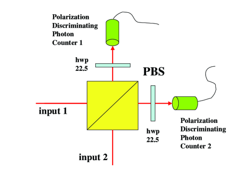
Figure 5: Schematic of a partial Bell state analyser. The polarization discriminating detectors would be constructed from additional polarizing beamsplitters (PBS) and photon counters in practice. If we find a single photon at each output and the polarization of the photons at each output are the same then the Bell state $|\phi^{+}\rangle$ has been identified. If the polarization of the photons at each output are different then $|\phi^{-}\rangle$ has been identified. If both photons are found at the top detector then the separable state $|HV\rangle$ has been identified. If both photons are at the bottom port then the separable state $|VH\rangle$ has been identified. hwp is a half-wave plate at the angle indicated.

The first demonstration of teleportation using these resources was by Bouwmeester et al. at the University of Innsbruck BOU97 . Their experiment used pulsed UV pumping of a non-linear crystal in a type II arrangement to produce pairs of polarization entangled photons at 788[nm] (2 and 3). The pump pulse was then retro-reflected through the crystal such that a second pair of counter-propagating photons (1 and 4) might be produced. Teleportation could then proceed by giving Alice entangled photon 2 and photon 1 as the teleportee (after it had been prepared in some arbitrary state) and giving Bob entangled photon 3. The fourth photon could be used as a trigger.

A simpler form of the partial Bell measurement was implemented by passing photons 1 and 2 through a 50/50 beamsplitter and then photon counting at the outputs. The action of a beamsplitter on the Bell states is to make the photons bunch (i.e. both exit through the same port). For all the Bell states that is except $|\psi-\rangle$, for which case the photons always exit by different ports. Thus if Alice records a coincidence count at the output of the beamsplitter then she has unambiguously identified the $|\psi-\rangle$ Bell state and teleportation has succeeded. The experiment is arranged such that the $|\psi-\rangle$ state is the “do nothing” result. If she does not obtain a coincidence the protocol has failed.

This experiment was very technically challenging. The probability of four photon events was very low. To prevent any temporal distinguishability of photons 1 and 2, a frequency filtering producing a 4[nm] bandwidth was applied, further reducing the counts. Finally the protocol itself only succeeded one quarter of the time. This resulted in roughly one successful event per minute. The fidelity with which the original states were reproduced was about $70\%$.

A sublety of the original experiment was that there was a significant probability for the down-converter to produce two photons each in modes 1 and 4. Then, even under perfect conditions of zero loss, a three-fold coincidence on Alice’s side of the experiment does not guarantee a photon is sent to Bob. In a later manifestation of the experiment the possibility of such errors was made negligible and fidelities of $>80\%$ were observed, well in excess of the $2/3$ limit PAN03 .

Teleportation can also be performed on single rail qubits. Here the Bell state can be produced by simply splitting a single photon on a 50:50 beamsplitter to give $|0\rangle|1\rangle+|1\rangle|0\rangle$. A Bell measurement is achieved also with a 50:50 beamsplitter and can successfully identify the two Bell states $|0\rangle|1\rangle\pm|1\rangle|0\rangle$. Again the other possibilities (two photons at one output) result in the measurement of the logical value of the qubit. A demonstration of single rail teleportation was carried out by Lombardi et al LOM02 .

Teleportation of coherent state qubits is also possible and has the unique property that deterministic Bell state analysis can be carried out with just a beamsplitter ENK02 ; JEO02 (provided the coherent states are sufficiently separated to be considered orthogonal, see section III.2). No experimental demonstration of this type of teleportation has yet been carried out.

As well as a method for quantum communication, all these types of teleportation can also be applied to quantum computation as will be highlighted in section VI.

V.2 Continuous Variable Teleportation

So far we have considered teleportation of qubits, as carried by the polarization degree of freedom of single photons. This technique will only work for single photon states. What if we wish to teleport a general field state with contributions from vacuum and higher photon number terms? The answer is to implement a teleportation protocol based on the measurement of the quadrature amplitudes of the field. Because the quadrature amplitudes are continuous, rather than discrete, variables, this is known as continuous variable (CV) teleportation. It was developed by Braunstein and Kimble BRA98 based on earlier work by Vaidman VAI94 .

Consider the situation depicted in Fig.6(a). Alice wishes to teleport to Bob an unknown coherent state, $|\alpha\rangle$, drawn from a broad Gaussian distribution. In the absence of entanglement Alice’s best approach is to divide the field into two equal parts at a beamsplitter and then measure the in-phase quadrature of one half and the out-of-phase quadrature of the other. The in-phase measurement gives an estimate of the real part of $\alpha$, whilst the out-of-phase measurement gives an estimate of the imaginary part of $\alpha$, however both estimates are imperfect due to noise from the vacuum field which inevitably enters through the open port of the beamsplitter. Alice sends these estimates to Bob who uses them to produce a coherent state by displacing his local vacuum state by the relevant quantities.

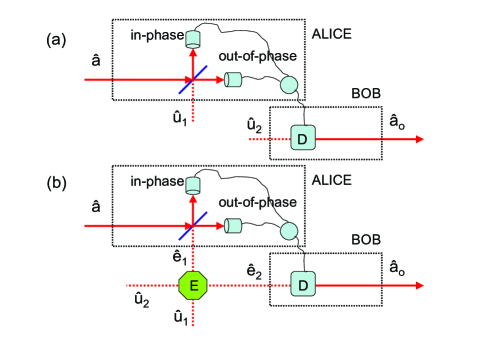
Figure 6: Schematic of continuous variable teleportation. In (a) is depicted the best strategy in the absence of entanglement. In (b) entanglement (E) is included in the protocol. Homodyne detection measures the in-phase and out-of-phase quadratures at Alice’s station. The results of the measurements are fed-forward to displace (D) Bob’s field.

This situation is most easily described in the Heisenberg picture. Let the initial field mode be represented by the annihilation operator ${\hat{a}}$ and the vacuum entering at the 50:50 beamsplitter by ${\hat{u}}_{1}$. The measurement results obtained by Alice are then represented by the quadrature operators

$${\hat{X}}^{+}_{a} = {{1}\over{\sqrt{2}}}({\hat{X}}^{+}_{a}-{\hat{X}}^{+}_{u1})$$

$${\hat{X}}^{-}_{a} = {{1}\over{\sqrt{2}}}({\hat{X}}^{-}_{a}+{\hat{X}}^{-}_{u1})$$ (36)

where $+$ ($-$) signifies the in-phase (out-of-phase) quadrature. These are sent to Bob who uses them to displace his vacuum field, ${\hat{u}}_{2}$ giving the output field

$${\hat{a}}_{o}={\hat{u}}_{2}+g{{1}\over{2}}({\hat{X}}^{+}_{a}+i{\hat{X}}^{-}_{a})-g{{1}\over{2}}({\hat{X}}^{+}_{u1}-i{\hat{X}}^{-}_{u1})$$ (37)

where $g$ is a gain factor for the displacement. Choosing $g=1$, unity gain, Bob’s output field is

$${\hat{a}}_{o}={\hat{a}}+{\hat{u}}_{2}-{\hat{u^{\dagger}}}_{1}$$ (38)

Notice that two vacuum fields have been added to the output, one entering through Alice’s measurement, the other through Bob’s reconstruction. Measurement of Bob’s quadrature amplitudes will show the same average value as Alice’s input: $\langle{\hat{X}}^{\pm}_{ao}\rangle=\langle{\hat{X}}^{\pm}_{a}\rangle$ as the vacuums have zero mean. On the other hand the quadrature variances of Bob’s state will be larger than the initial state:

$$V_{ao} = \langle({\hat{X}}^{\pm}_{ao})^{2}\rangle-\langle{\hat{X}}^{\pm}_{ao}\rangle^{2}$$ (39)

$$= \langle({\hat{X}}^{\pm}_{a})^{2}\rangle+\langle({\hat{X}}^{\pm}_{u1})^{2}\rangle+\langle({\hat{X}}^{\pm}_{u2})^{2}\rangle-\langle{\hat{X}}^{\pm}_{a}\rangle^{2}$$

$$= 3$$

As a result Bob’s state is mixed (no longer minimum uncertainty) and is 3 times noisier than the QNL level of the input coherent state.

Now suppose Alice and Bob share an entangled state. In particular we assume they share an EPR entangled state REI88 ; OU92 named after the famous paradox proposed by Einstein, Podolsky and Rosen EIN35 . This state, also commonly known as a two mode squeezed state, exhibits strong correlations between both the in-phase and out-of-phase quadratures of its component beams. It can be described by its Heisenberg evolution:

$${\hat{u}}_{1} \to \sqrt{G}\;{\hat{u}}_{1}+\sqrt{G-1}\;{\hat{u}}_{2}^{\dagger}$$

$${\hat{u}}_{2} \to \sqrt{G}\;{\hat{u}}_{2}+\sqrt{G-1}\;{\hat{u}}_{1}^{\dagger}$$ (40)

where ${\hat{u}}_{i}$ are initially vacuum states and $G$ is the parametric gain (or squeezing). This interaction is produced by parametric amplification WU87 either directly by a non-degenerate system or alternatively via degenerate parametric amplification (ie squeezing) followed by the out-of-phase mixing of the two modes on a 50:50 beamsplitter. A non-degenerate parametric amplifier is basically just a high efficiency down converter as can be seen from the Scrödinger picture evolution equivalent to Eq.40:

$$|EPR\rangle = {{1}\over{\sqrt{G}}}\;\;(|0\rangle_{1}|0\rangle_{2}+{{\sqrt{G-1}}\over{\sqrt{G}}}|1\rangle_{1}|1\rangle_{2}$$ (41)

$$+ \left({{\sqrt{G-1}}\over{\sqrt{G}}}\right)^{2}|2\rangle_{1}|2\rangle_{2}+\ldots..)$$

Alice again divides and measures her beam but this time instead of allowing vacuum to enter the empty port of her beamsplitter she sends in her half of the EPR pair. As a result her quadrature measurement results are now given by

$${\hat{X}}^{+}_{a} = {{1}\over{\sqrt{2}}}({\hat{X}}^{+}_{a}-\sqrt{G}\;{\hat{X}}^{+}_{u1}-\sqrt{G-1}\;{\hat{X}}^{+}_{u2})$$

$${\hat{X}}^{-}_{a} = {{1}\over{\sqrt{2}}}({\hat{X}}^{-}_{a}+\sqrt{G}\;{\hat{X}}^{-}_{u1}-\sqrt{G-1}\;{\hat{X}}^{-}_{u2})$$ (42)

where we have used equation (40) to describe the entanglement. These results are sent to Bob who now uses them to displace his half of the EPR pair, obtaining (at unity gain)

$${\hat{a}}_{o}={\hat{a}}+(\sqrt{G}-\sqrt{G-1}){\hat{u}}_{2}+(\sqrt{G}-\sqrt{G-1}){\hat{u^{\dagger}}}_{1}$$ (43)

Now in the limit $G\to\infty$, $(\sqrt{G}-\sqrt{G-1})\to 0$, hence in this limit equation (43) reduces to

$${\hat{a}}_{o}={\hat{a}}$$ (44)

Evolution through the teleporter is the identity and so the output state is identical to the input (this is obviously true not only for the coherent input states we have been considering but for any input state).

The first demonstration of this type was made by Furusawa et al. FUR98 . EPR entanglement was produced by the mixing of two out-of phase squeezed beams on a 50/50 beamsplitter. Both squeezed beams (at 860[nm]) were generated in a single ring-cavity parametric oscillator by simultaneously pumping counter-propagating cavity modes. One of the EPR beams was sent to Alice who mixed it with her signal beam and performed dual balanced homodyne measurements, actively locked to be 90 degrees out of phase, such that conjugate quadrature measurements were made. The photo-currents thus generated are sent to Bob who uses them to impose phase and amplitude modulations on a bright laser beam. By mixing this bright beam with his EPR beam on a highly reflective beamsplitter Bob can efficiently impose on the EPR beam a displacement proportional to the modulations. All the beams in the experiment originate from a single Ti:Sapph master laser, including the signal beam which has a known modulation amplitude (effectively the coherent amplitude of the coherent state) imposed on it before being sent to Alice. When, based on the signal size observed on Bob’s side, unity gain was achieved, the quadrature noise floors of the teleported beam were measured by an independent balanced homodyne detector, both with and without entanglement.

The quality of Bob’s reconstruction can be evaluated via the fidelity of it compared with the initial coherent state Alice sent (see Eq.29). Provided the output is Gaussian (which it is) this fidelity is given by

$$F = {{2}\over{\sqrt{(V^{+}_{ao}+1)(V^{-}_{ao}+1)}}}$$ (45)

$$\times \exp\left[-{{2}\over{\sqrt{(V^{+}_{ao}+1)(V^{-}_{ao}+1)}}}|\alpha|^{2}(1-g)^{2}\right]$$

Recalling from our earlier discussion that without entanglement the quadrature variances of the outputs are $V^{+}_{ao}=V^{-}_{ao}=3$, then we find from equation (45) that for large $\alpha$ the best fidelity with no entanglement is achieved at unity gain and is $F=0.5$. This is confirmed by Furusawa et al who find a best fidelity without entanglement of $F_{c}=0.48\pm 0.03$. On the other hand, with entanglement, a fidelity of $F_{q}=0.58\pm 0.02$ is measured, clearly exceeding the classical bound.

A subsequent experiment by Bowen et al BOW03 . achieved higher fidelities ($F_{q}=0.64\pm 0.02$) and stable operation over long periods. Their experiment used two independent, monolithic, sub-threshold parametric oscillators to produce twin squeezed beams at 1064 [nm] which were then mixed on a beamsplitter to produce the required EPR entanglement.

The performance of the Bowen et al teleporter was also characterised in terms of the signal to noise transfer ($T$) and the conditional variance ($V$) between the input and output fields: the teleportation T-V diagram RAL98 . As we have seen, in the absence of entanglement strict bounds are placed on both the accuracy of measurement and reconstruction of an unknown state. These are represented by the vacuum modes that appear in equation (38). These bounds can be quantified in the following way.

Alice’s measurement accuracy is limited by the generalized uncertainty principle of Arthurs and Goodman, $V^{+}_{M}V^{-}_{M}\!\geq\!1$ ART88 , where $V+_{M},V^{-}_{M}$ are the quadrature measurement penalties, which holds for any simultaneous measurements of conjugate quadrature amplitudes of an unknown quantum optical system. For Gaussian input states this relationship can be re-written in terms of quadrature signal transfer coefficients, $T^{+}={S/N}^{+}_{\rm out}/{S/N}^{+}_{\rm in}$ and $T^{-}={S/N}^{-}_{\rm out}/{S/N}^{-}_{\rm in}$ as

$$T_{q}=T^{+}+T^{-}-T^{+}\;T^{-}\left(1-\frac{1}{V^{+}_{in}V^{-}_{in}}\right)\leq 1$$ (46)

where ${S/N}^{+}$ (${S/N}^{-}$) is the signal-to-noise ratio of the in-phase (out-of-phase) quadratures. This expression reduces to $T_{q}=T^{+}+T^{-}$ for minimum uncertainty input states ($V^{+}_{in}V^{-}_{in}=1$). Without entanglement it is not possible to break the inequality given in equation (46).

Bob’s reconstruction must be carried out on a mode of the E/M field the fluctuations of which must already obey the uncertainty principle. In the absence of entanglement these intrinsic fluctuations remain present on any reconstructed field, thus the amplitude and phase conditional variances, $V^{+}_{{\rm in|out}}\!=\!V^{+}_{{\rm out}}\!-\!|\langle\delta\hat{X}^{+}_{{\rm in}}\delta\hat{X}^{+}_{{\rm out}}\rangle|^{2}\!/V^{+}_{{\rm in}}$ and $V^{-}_{{\rm in|out}}\!=\!V^{-}_{{\rm out}}\!-\!|\langle\delta\hat{X}^{-}_{{\rm in}}\delta\hat{X}^{-}_{{\rm out}}\rangle|^{2}\!/V^{-}_{{\rm in}}$ respectively, which measure the noise added during the teleportation process, will satisfy $V_{q}=V^{+}_{{\rm in|out}}V^{-}_{{\rm in|out}}\!\geq\!1$. For Gaussian input states this can be written in terms of the signal transfer and quadrature variances of the output state as

$$V_{q}=(1-T^{+})(1-T^{-})\;V^{+}_{\rm out}V^{-}_{{\rm out}}\;\geq 1$$ (47)

The criteria of equations (46) and (47) can then used to represent quantum teleportation on a T-V graph. An important feature of the T-V criteria is that it can characterize teleportation at non-unity gains RAL99 .

The $T_{q}$ and $V_{q}$ bounds have independent physical significance. If Bob’s state passes the $T_{q}$ bound (equation (46)) then he can be sure, regardless of how it was transmitted to him, that no other party can possess a copy of the state which also passes this bound (ie carries as much information about the original). Surpassing the $V_{q}$ bound is a necessary prerequisite for reconstruction of non-classical features of the input state such as squeezing or negativity of the Wigner function. Clearly it is desirable that the $T_{q}$ and $V_{q}$ bounds are simultaneously exceeded, thus demonstrating fully quantum operation. The cross-over point (1,1), corresponds to a fidelity of $2/3$. The significance of crossing this boundary has been investigated by a number authors GRO01 ; CAV04 . Perfect reconstruction of the input state would result in $T_{q}\!=\!2$ and $V_{q}\!=\!0$. In the Bowen et al experiment a number of results were obtained that passed the $T_{q}$ bound and one point (marginally) exceeded both $T_{q}$ and $V_{q}$ simultaneously.

More recently Takei et al TAK05 conclusively demonstrated passage into the fully quantum region by obtaining a fidelity of $0.7$ and realizing entanglement swapping at unity gain. The experiment was carried out with an array of 4 parametric oscillators operating at 860 [nm]. By combining pairs of beams, 2 strongly entangled EPR sources were created. One beam from the first EPR source was teleported by the second EPR source. By looking for correlations between the teleported beam and the other beam of the first source it could be established that they were still entangled. The input beam represented a good approximation to an unknown state and the preservation of entanglement showed that quantum features of the state could be successfully transferred.

VI Quantum Computation

We have now examined a number of quantum information tasks that have been achieved using optics. We have seen that with some encodings arbitrary control of single qubits can be achieved and specific entangled states can be produced and used as resources for small scale operations. But what about the more challenging task of quantum computation? The skills so far discussed are insufficient to implement quantum computation. It turns out that to be able to implement arbitrary processing of information encoded on a set of qubits it is sufficient to possess at least one non-trivial two qubit operation, in addition to arbitrary operations on single qubits.

An example of a non-trivial two-qubit gate is the CNOT gate. In terms of polarisation qubits its operation is summarised by the following truth table

$$|H\rangle_{c}|H\rangle_{t} \to |H\rangle_{c}|H\rangle_{t}$$

$$|H\rangle_{c}|V\rangle_{t} \to |H\rangle_{c}|V\rangle_{t}$$

$$|V\rangle_{c}|H\rangle_{t} \to |V\rangle_{c}|V\rangle_{t}$$

$$|V\rangle_{c}|V\rangle_{t} \to |V\rangle_{c}|H\rangle_{t}$$ (48)

When the control qubit is in the horizontal state, $|H\rangle_{c}$, the value of the target qubit $|H\rangle_{t}$ or $|V\rangle_{t}$ is unchanged. However, when the control is vertical, $|V\rangle_{c}$, the value of the target qubit is flipped, horizontal to vertical and vice versa. The effect of a CNOT gate on superposition states is simply a superposition of the transformations of equation (48). For example if the control is in the diagonal basis we get the following transformations

$$(|H\rangle_{c}+|V\rangle_{c})|H\rangle_{t} \to (|H\rangle_{c}|H\rangle_{t}+|V\rangle_{c}|V\rangle_{t})$$

$$(|H\rangle_{c}+|V\rangle_{c})|V\rangle_{t} \to (|H\rangle_{c}|V\rangle_{t}+|V\rangle_{c}|H\rangle_{t})$$

$$(|H\rangle_{c}-|V\rangle_{c})|H\rangle_{t} \to (|H\rangle_{c}|H\rangle_{t}-|V\rangle_{c}|V\rangle_{t})$$

$$(|H\rangle_{c}-|V\rangle_{c})|V\rangle_{t} \to (|H\rangle_{c}|V\rangle_{t}-|V\rangle_{c}|H\rangle_{t})$$ (49)

Notice that the resulting output states are the four Bell-states, see section (V). If we run this interaction back-wards, that is input the Bell states, we see that orthogonal, separable states are outputted, hence enabling efficient Bell-state analysis. Thus the CNOT gate is a very useful device even for small-scale applications. So how might such an interaction between two photons be implemented? One solution is to use a $\chi_{3}$ non-linear medium to induce a cross-Kerr effect between two photon modes, as first suggested by Milburn MIL89 . Ideally the cross-Kerr effect will produce the unitary evolution ${\hat{U}}_{K}=\exp[i\chi{\hat{a}}^{\dagger}{\hat{a}}{\hat{b}}^{\dagger}{\hat{b}}]$, where ${\hat{a}}$ represents one optical mode and ${\hat{b}}$ another. Consider the schematic set-up of Fig.7. Two polarization encoded qubits are converted into spatial dual rail qubits using polarizing beamsplitters. One mode from each of the qubits is sent through the cross-Kerr material. The operation of this device on an arbitrary two qubit input state is given by the following evolution:

$$|\psi\rangle \to {\hat{U}}_{K}|\psi\rangle$$

$$= e^{i\chi{\hat{a}}_{2}^{\dagger}{\hat{a}}_{2}{\hat{b}}_{1}^{\dagger}{\hat{b}}_{1}}(\alpha|01\rangle_{a}|01\rangle_{b}+\beta|10\rangle_{a}|10\rangle_{b}$$

$$\;\;\;\;\;\;\;\;\;\;\;\;\;\;\;\;\;\;\;\;\;\;\;\;\;+\gamma|10\rangle_{a}|01\rangle_{b}+\delta|01\rangle_{a}|10\rangle_{b})$$

$$= \alpha|01\rangle_{a}|01\rangle_{b}+\beta|10\rangle_{a}|10\rangle_{b}$$

$$\;\;\;\;\;\;\;\;\;\;\;\;\;\;\;\;\ +\gamma|10\rangle_{a}|01\rangle_{b}+e^{i\chi}\delta|01\rangle_{a}|10\rangle_{b}$$

Only when both modes entering the Kerr material are occupied is a phase shift induced. If we now choose the strength of the non-linearity such that $\chi=\pi$, the effect is to flip the sign of one element of the superposition. This is called a controlled-sign (CS) gate. If Hadamard gates are placed on qubit $b$, before and after the CS gate (as could be implemented with wave plates, see section III.1) then CNOT operation is achieved with qubit $a$ as the control and qubit $b$ as the target.

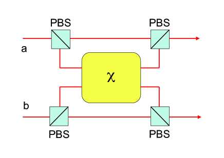
Figure 7: Schematic of the implementation of an optical CS gate using a strong cross-Kerr non-linearity $\chi$. PBS are polarizing beamsplitters.

The problem with this idea in practice is that typical non-linear materials have values of $\chi$ that are an order of magnitude of orders of magnitude too small. One might consider making the interaction region of the material very long in order to boost the non-linearity, but such a strategy generally leads to very high levels of loss, which negate the desired effect. Non-linearities close to those required can be realized in cavity quantum electro-dynamic (QED) situations featuring single atoms in cavities of extremely high finesse and small volume BRU96 ; TUR95 . This occurs in the so-called strong coupling regime, in which the dipole coupling between the cavity field and the atom is significantly greater than the relaxation rates of both the cavity and the dipole. Many problems exist with this approach including: the difficulty of coupling photons efficiently into and out of the cavity mode; the need to isolate the cross-Kerr non-linearity from other non-linear effects and; the difficulty in maintaining a constant coupling strength between the atom and the field. A number of ingenious solutions have been suggested DUA04 ; NEM04 but remain unproven experimentally to date.

These problems led most to conclude that large scale quantum processing with optics was untenable. However a number of results in the late nineties and early noughties, culminating in the 2001 paper by Knill, Laflamme and Milburn (KLM) KNI01 led many to change their view. KLM found a way to circumvent the problem of needing a huge non-linearity and showed that it was possible to implement efficient quantum computation using only passive linear optics, photodetectors, and single photon sources. In the following we will first describe how Grover’s quantum algorithm can be implemented in a straight forward manner using linear optics. We then describe KLM’s more ambitious scheme for general quantum computation and the experimental steps that have so far been taken.

VI.1 Grover’s Algorithm

Grover’s algorithm GRO97 is an important algorithm in quantum computation giving a provable speed-up over classical algorithms in searching an unstructured data-base. The best classical algorithm for finding a single marked item in an unstructured data base is to simply randomly sample. On average, it will take $N/2$ attempts to find the item. Quantum information allows a better solution which is depicted in Fig. 8(a). Dependent on the logical state of a qubit bus a quantum oracle samples the data base. If the nominated item is found, the qubit bus is marked by a phase flip, otherwise the qubit bus is left unchanged. By placing the qubit bus in an equal superposition of all logical states all the data base states can be interogated by a single oracle call. The result is an equal superposition output state with a single phase flip against the qubit state corresponding to the marked item. Inversion about the mean is then performed on the qubit bus, which has the effect of amplifying the marked item with respect to the others. After iterating this process for order $\sqrt{N}$ times the item can found with high accuracy by a measurement on the qubit bus in the computational basis. Although not an exponential speed-up, the improvement in search speed can be quite significant for large $N$. In Fig. 8(b) we show explicitly the smallest non-trivial example: a 4 element data base. In this case a single iteration is sufficient to determine the marked element with unit probability.

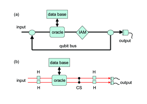
Figure 8: Schematic representations of the implementation of Grover’s algorithm. (a) General case showing basic flow structure. IAM stands for inversion about the mean. The iterative step is carried out of order $\sqrt{N}$ times, where $N$ is the size of the unstructured data base. (b) Specific implementation for case of $N=4$. The qubits are input in the state $|\bf 0\bf 0\rangle$ and the output is measured in the computational basis. The 4 possible separable output states unambiguously identify the 4 possible tagged elements with a single query. CS indicates a CS gate and H indicates Hadamard gates.

We will now consider the implementation of Grovers algorithm in optics. The oracle plays a key role in search algorithms so we shall begin by describing how, in general, a search oracle can be implemented in optics. Initially we will assume that CNOT gates operating on the principle of Eq.LABEL:c-K are available. We will additionally use the feature that the action of the gate on an unoccupied (vacuum) target mode leaves both modes unchanged, that is

$$\alpha_{1}|H\rangle|0\rangle+\alpha_{2}|V\rangle|0\rangle\to\alpha_{1}|H\rangle|0\rangle+\alpha_{2}|V\rangle|0\rangle$$ (51)

where $0$ represents the vacuum. We will then show the rather surprising result that such gates are not in fact required in order to implement Grover’s algorithm.

VI.1.1 The Oracle

We require that the oracle, when queried by some $n$ qubit state will query the corresponding element of an unstructured $2^{n}=N$ element classical data-base and either return the same $n$ qubit state (if the element is not tagged) or a phase flipped version (if the element is tagged). We assume the simplest case that only one element is tagged. In order that superpositions of the input state should be preserved it is clear that we need a classical data-base which can be interogated by a quantum particle. Optics provides a straightforward solution to this problem.

To illustrate the technique we shall begin by considering an oracle querying a 4 element data-base. We will then generalize the result. The proposed arrangement is shown in Fig.9. The classical data-base is comprised of a piece of glass partioned into four domains. One of the domains (representing the tagged element) has an optical pathlength which is $\lambda/2$ longer than the pathlengths of the other domains. Here $\lambda$ is the optical wavelength.

The principle of the oracle is to direct a single photon through one of the four domains as a function of the state of a 2 qubit input. If it traverses the tagged domain it will pick up a $\pi$ phase shift relative to passage through the other domains. Path information carried by the single photon is then erased via a measurement protocol leaving the phase flip on the corresponding 2 qubit state. Because the photon is a quantum particle it can be placed into a superposition of traversing various domains simultaneously.

We start with the qubits in an arbitrary superposition state and the “oracle photon” in the horizontal state:

$$|H\rangle(\alpha_{1}|H\rangle|H\rangle+\alpha_{2}|H\rangle|V\rangle+\alpha_{3}|V\rangle|H\rangle+\alpha_{4}|V\rangle|V\rangle)$$ (52)

Here the ordering of the kets from left to right in Eq.52 corresponds to the rail sequence from top to bottom in Fig.9.

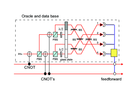
Figure 9: Schematic of oracle for 4-bit data base. PBS are polarising beamsplitters whilst BS are 50:50 non-polarising beamsplitters. The dashed line on the beamsplitters indicates the surface from which reflection induces a sign change. Polarising beamsplitters are assumed to reflect the horizontal component and transmit the vertical component of the incident light. Half-wave-plates are indicated by $\lambda/2$ and are oriented at 45 degrees to horizontal, thus flipping the polarization of the incident beam. Single lines indicate optical rails whilst double lines indicate electrical rails. See text for description of operation.

Next a CNOT gate with the first qubit as the control and the oracle photon as the target is applied. Depending on the value of the first qubit the polarization of the photon is either left alone or flipped to $V$. The oracle photon then passes through a polarizing beamsplitter which separates the polarization modes into two separate spatial paths. We now apply CNOT’s with the second qubit as their control and each of the new oracle photon spatial modes as targets. Subsequent polarizing beamsplitters again divide polarization modes into different spatial modes resulting in four different paths that the photon can take. Each of the different paths is uniquely determined by one of the four possible logical basis input states of the qubit. Thus the state of the system has now evolved to:

$$\alpha_{1}|p_{1}\rangle|H\rangle|H\rangle + \alpha_{2}|p_{2}\rangle|H\rangle|V\rangle$$ (53)

$$+ \alpha_{3}|p_{4}\rangle|V\rangle|H\rangle+\alpha_{4}|p_{3}\rangle|V\rangle|V\rangle$$

where we have used the $|p_{1}\rangle\equiv|1,0,0,0\rangle$, $|p_{2}\rangle\equiv|0,1,0,0\rangle$, etc. The oracle photon then passes through the glass plate data base. For concreteness we will assume that it is the first domain which has the increased path length, thus the state of the system after the interaction with the data base is

$$-\alpha_{1}|p_{1}\rangle|H\rangle|H\rangle + \alpha_{2}|p_{2}\rangle|H\rangle|V\rangle$$ (54)

$$+ \alpha_{3}|p_{4}\rangle|V\rangle|H\rangle+\alpha_{4}|p_{3}\rangle|V\rangle|V\rangle$$

The tag has successfully been attached to the qubit state however the oracle photon still carries information about the qubit state which must be erased. This could be done by reversing the sequence of gates used before the data-base as was suggested by Nielsen and Chuang NIE00 . However, the need for more quantum gates can be avoided by employing a measurement based erasure protocol. This is achieved by mixing all the possible photon paths on 50:50 beamsplitters. There is then an equal probability of finding the photon in any of the four paths, thus erasing the qubit information. The photon is then detected. Depending on where the photon is found the following phase corrections must be made to the qubits: (i) If the photon is counted at detector 1, do nothing; (ii) if the photon is counted at the second detector then a phase shift (defined by $Z|H\rangle=|H\rangle$, $Z|V\rangle=-|V\rangle$ and implementable with a quarter-wave plate) is applied to qubit 2; (iii) if the photon is counted at the third detector then a phase shift is applied to both qubits and; (iv) if the photon is counted at the fourth detector then a phase shift is applied to the first qubit. After the correction has been made the qubits are left (up to a global phase factor) in the state

$$-\alpha_{1}|H\rangle|H\rangle+\alpha_{2}|H\rangle|V\rangle+\alpha_{3}|V\rangle|H\rangle+\alpha_{4}|V\rangle|V\rangle$$ (55)

which is the required state.

This scheme is easily generalized to larger data-bases. For example to search an eight element data-base we require a three qubit register and a glass plate with eight domains. The first two steps of the protocol run the same as before with the photon being fanned out to four different paths. Now four CNOT’s, all controlled by the third qubit and with the four photon paths as their respective targets, direct the oracle photon into eight possible paths, each uniquely determined by the qubit values. The paths are passed through the data-base, resulting in tagging, and the qubit information is erased by mode mixing followed by detection in an analogous way to the four element protocol. It is clear that the scheme can be further expanded in this way to any finite sized data-base. In general the oracle will require $(N-1)$ CNOT gates where $N=2^{n}$ is the data-base size and $n$ is the number of qubits in the register.

VI.1.2 Grover’s Algorithm with Linear Optics

In the previous section we showed how a search oracle could in general be implemented in an optical quantum computation circuit, given a cross-Kerr type two-qubit gate. We now consider the specific case of Grover’s algorithm and show that in fact the entire algorithm can be performed using only linear optics.

Consider the initial interaction between the qubit bus and the oracle. In Grover’s this step is used to instruct the oracle to make an equal superposition query of all data base elements. However, this can be achieved using only linear optics by simply fanning out a single photon mode into $N$ modes using 50:50 beamsplitters. After the oracle the result is read to the qubit bus for the processing step of inversion about the mean. After processing it is read back to the oracle that then queries the data base again. But actually it is unnecessary to read the information back to a qubit bus in order to perform the processing. As shown by Kwiat and Zeilinger REC94 , any unitary operation can be performed on a unary data bus using only linear optics. A unary data bus is one in which a particular number, $n$, is represented by having the $nth$ bit flipped with respect to all the others. For the optical bus this is represented in single rail logic (see section III.2) by having only the $nth$ mode occupied by a single photon. This is in contrast to a binary data bus in which $n$ would be represented by the binary digit $n_{base2}$.

In a general quantum computation circuit such a unary encoding would lead to an exponential expense in the number qubits needed in comparison to a binary encoding and would in most cases quickly nullify any gain made through the quantum approach. However, for the specific case of a search algorithm like Grover’s, it is a required step to introduce a unary qubit bus in order that the unstructured data base can be queried. It is thus of no benefit to continually shift back and forth between the binary and unary qubit buses and is just as efficient to remain in the unary qubit bus and perform all the processing using linear optics.

A number of groups have performed in principle demonstrations of Grover’s algorithm using linear optics. Kwiat el al KWI99 searched a 4 element data base. They used a combination of polarization and spatial encoding to form the unsorted data bus and a Sagnac interferometer to form a passively stable interferometric arrangement. The data base was electro-optically ”programmed” via waveplates and a Pockell cell. They achieved around 90% probability of successfully identifying the marked data base element. Bahattacharya et al BAH02 , motivated by a proposal of Lloyd LLO00 , were able to search up to a  32 element data base, represented by a thin groove in glass plate. They used a standing-wave cavity to achieve repeated interactions with the data base and Fourier optics to produce the required inversions about the mean.

In neither of these experiments were single photon states used. Rather, bright optical pulses containing huge numbers of photons passed through the systems. Although in the case of the Kwiat experiment it would have been reasonably straightforward to run the experiment with single photons NOTE1 , a significantly more difficult set-up would be required to allow the Bahattacharya experiment to be run with any reasonable efficiency in the single photon domain. This prompts the question of whether, if the basic effect of Grover’s algorithm is observable with bright beams of light, the algorithm should be considered ”quantum”. We now briefly address this question.

VI.1.3 Is Grover’s Algorithm Quantum?

In order to answer the question ”Is Grover’s Algorithm Quantum?” we first need to define what we mean by ”a single query of the data base” and what we mean by ”quantum”. We will adopt the following definitions:

1. A single query of the data base occurs when, on average, a single photon interacts with the data base.

2. The algorithm will be considered quantum if it is necessary for entanglement to exist between the optical modes comprising the unsorted data bus in order to achieve the $\sqrt{N}$ scaling.

Notice that by this definition neither of the experiments so far performed strictly realized Grover’s algorithm as both involved many photons interacting with the oracle per query. We now consider three examples that satisfy the query definition, two of which involve entanglement and one of which does not.

Firstly, the implementation of the oracle represented in Fig. 9 clearly satisfies the query definition and also produces a $\sqrt{N}$ scaling. The state of the data bus just before the first interaction with the data base is

$$|\psi\rangle=|100...00\rangle+|010...00\rangle+.....|000...01\rangle$$ (56)

which clearly exhibits modal entanglement.

Can we remove the entanglement and still retain the $\sqrt{N}$ scaling. As a second example we could consider using a weak coherent state with amplitude $\alpha=1$ as the input instead of a single photon state. We still satisfy the query requirement on average and the algorithm still achieves a $\sqrt{N}$ scaling. Because we are using a weak coherent state there is a $37\%$ probability for any particular query that we will inject vacuum into the circuit and hence get a null result. However this efficiency is constant, independent of the size of the data base and thus does not affect the scaling. Is there still entanglement present? At first sight the answer to this question may appear to be ”no”, as the unitary evolution of a coherent state through a beamsplitter does not produce entanglement. However the photon counters used to detect the final state have microscopic resolution and reject the vacuum state realizations. As a result, on the occasions the algorithm succeeds, the detectors post-select circuit states similar to that in Eq.56. Again, entanglement is seen to be present.

To avoid both unitary and post-selected entanglement we consider a third example in which again we use a weak coherent state with amplitude $\alpha=1$ as the input but now use homodyne detection of the final state. Homodyne detection measures the field amplitude and so does not resolve individual quanta. As a result it cannot post-select entanglement from coherent state inputs. Now the state of the data bus just before the first interaction with the data base is

$$|\psi\rangle=|\alpha^{\prime},\alpha^{\prime},...,\alpha^{\prime}\rangle$$ (57)

where $\alpha^{\prime}=1/\sqrt{N}$. Eq.57 is clearly a separable state. The output state after the correct number of iterations will be approximately

$$|\psi\rangle_{out}=|0,0,..,\alpha,...,0\rangle$$ (58)

where the mode position of the displaced state gives the marked element. However, using homodyne detection means that there is vacuum noise associated with the unoccupied modes meaning we cannot unambiguously identify the marked element. Indeed the signal to noise with which we can identify the correct element is now $1/N$. In order to maintain a constant signal to noise, say of $1$, we need to repeat the algorithm $\sqrt{N}$ times. As a result we find that the number of data base queries scales with $N$ in this case, just as for the classical algorithm. Given our energy constraint it is hard to imagine how this problem can be avoided whilst still maintaining separable states.

These examples suggest strongly that, given our definitions, Grover’s algorithm should be considered a quantum algorithm not-with-standing its classical field analogues.

VI.2 Linear Optical Quantum Computation

As we have already mentioned, it is not possible to construct a general quantum computation network using the unsorted encoding scheme without incurring an exponential overhead. In the following we will describe the scheme of KLM, in which the standard dual-rail qubit encoding is used, but arbitrary processing is achieved without Kerr type non-linearity or an exponential overhead. Instead the KLM toolbox comprises: single photon sources; photon counting detectors and; electro-optic feed-forward.

There are three tiers to the KLM scheme:

1. Non-deterministic two qubit gates which can be used to produce entangled resource states.

2. Non-deterministic teleportation gates which are driven by entangled resource states and fail by accidentally measuring the value of the qubit.

3. Error correcting codes that protect the qubits from accidental measurement during the application of the teleportation gates and hence allow scale up of universal circuits without an exponential overhead.

We now discuss each of these tiers in turn and the experimental progress that has been made towards quantum computing based on this paradigm.

VI.2.1 Non-Deterministic Entangling Gates

At the first level, KLM introduced two qubit gates that could take separable, single photon inputs, and produce entangled outputs. In particular KLM showed how to make a CNOT gate that was non-deterministic, but heralded. That is, the gate does not always work, but an independent signal heralds successful operation. A somewhat simplified version of this gate is shown in Fig.(10) RAL01 . In addition to the single photon, polarisation qubits incident at ports $c$ (control) and $t$ (target), the gate also has ancilla inputs comprising two vacuum input ports, $v1$ and $v2$, and two single photon input ports, $p1$ and $p2$. The beamsplitter reflectivities are given by $\eta_{1}=5-3\sqrt{2}$ and $\eta_{2}=(3-\sqrt{2})/7$. It can be shown that when no photons are detected at outputs $vo1$ and $vo2$, and one and only one photon is detected at each of $po1$ and $po2$, then the gate has succeeded and the photon qubits exiting through $co$ and $to$ have had the CNOT transformation applied to them. The probability of successful operation is $\eta_{2}^{2}\approx 0.05$. Recently it has been proved by Eisert EIS05 that $1/16$ is the upper bound for success probability for a gate of this type (as achieved by the original KLM proposal).

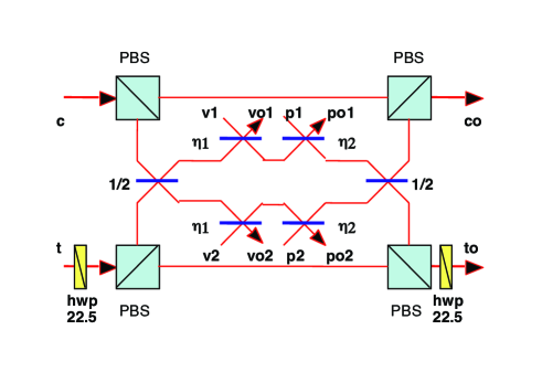
Figure 10: Schematic representation of a non-deterministic CNOT gate. Polarization encoded qubits are injected at $c$ and $t$. Acillary photons are injected at $p1$ and $p2$. Successful operation is heralded by the detection of no photons at outputs $vo1$ and $vo2$ and the detection of one and only one photon at each of outputs $po1$ and $po2$. PBS are polarizing beamsplitters and hwp are half-wave plates.

Even at this first level the technical requirements are demanding. Four photons need to simultaneously enter the circuit. The detections at $po1$ and $po2$ have to distinguish between zero, one or two photons. Any inefficiency in the production or detection of photons will lead to mistakes and rapidly erase the operation of the gate. High visibility single photon and two photon (HOM type) interference are required simultaneously: as a result excellent mode-matching and photon indistinguishability are essential.

A significantly simpler CNOT design can be realised by working in coincidence as discussed by Ralph et al RAL02 and independently by Hofmann and Takeuchi HOF02 . In particular we can allow the photon qubits to be their own ancilla, such that only two photons are required. The gate is shown schematically in Fig.(11). Consider the input $|H\rangle_{c}|H\rangle_{t}$. The target waveplate produces the transformation

$$|H\rangle_{c}|H\rangle_{t}\to{{1}\over{\sqrt{2}}}|H\rangle_{c}(|H\rangle_{t}+|V\rangle_{t})\\$$

The polarizing beamsplitters then spatially separate the polarization modes of the two beams. An array of different possibilities are present after the middle beamsplitters, however, we select (by postselection) only those where a photon arrives at both the target and control outputs. There are two ways for this to happen: the control photon must take the top path and reflect off beamsplitter 1; the target photon may take its upper path and reflect off beamsplitter 2 or take the bottom path and reflect off beamsplitter 3. In both cases the effect is just to reduce the amplitude of the successful components by a factor of $1/3$. The output state is then transformed by the second target waveplate such that

$${{1}\over{3}}{{1}\over{\sqrt{2}}}|H\rangle_{c}(|H\rangle_{t}+|V\rangle_{t})\to{{1}\over{3}}|H\rangle_{c}|H\rangle_{t}\\$$

Similarly the input $|H\rangle_{c}|V\rangle_{t}$ is unchanged by passage through the circuit, other than a $1/3$ reduction in amplitude.

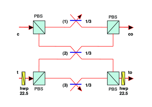
Figure 11: Schematic representation of non-deterministic coincidence CNOT gate. Polarization encoded qubits are injected at $c$ and $t$. PBS are polarizing beamsplitters and hwp are half-wave plates.

Things are different when the control is in the vertical state. Consider the input state $|V\rangle_{c}|H\rangle_{t}$. The target waveplate produces the transformation

$$|V\rangle_{c}|H\rangle_{t}\to{{1}\over{\sqrt{2}}}|V\rangle_{c}(|H\rangle_{t}+|V\rangle_{t})\\$$

Now there are three ways for a successful detection to occur. The control takes its lower path. If the target photon takes the bottom path then both must reflect off their respective beamsplitters as before, simply reducing the amplitude by $1/3$. However, if the target photon follows its upper path then there are two possibilities at beamsplitter 2: either both photons may be reflected, giving an amplitude of $1/3$, or; both may be transmitted, giving an amplitude of $-2/3$. If the photons are indistinguishable then these amplitudes are added giving a total amplitude for that component of $-1/3$! Thus when the polarization modes are recombined the state carries a minus sign on one target component and the second target waveplate makes the transformation

$${{1}\over{3}}{{1}\over{\sqrt{2}}}|V\rangle_{c}(|H\rangle_{t}-|V\rangle_{t})\to{{1}\over{3}}|V\rangle_{c}|V\rangle_{t}\\$$

and the value of the target qubit is flipped as required. Similarly the circuit does the transformation $|V\rangle_{c}|V\rangle_{t}\to 1/3|V\rangle_{c}|H\rangle_{t}$. Hence CNOT operation is realized whenever a coincidence is recorded. The probability of success is $(1/3)^{2}=1/9$.

J.O’Brien and G.Pryde et al used this technique to demonstrate CNOT operation for single photon qubits OBR03 . In their experiment a pair of polarisation beam displacers was used to create an interferometrically stable configuration. Down conversion was used to produce suitably pure photon pairs in separable polarization states which were injected into the gate. State tomography (see section III.5) was used to compare the experimental output with the expected outcome. Good agreement was found. In particular entanglement could be produced as expected. In later experiments full process tomography was carried out OBR04 from which an average fidelity of around 90% for the gate was calculated.

VI.2.2 Teleportation Gates

We now proceed to the second tier of the KLM scheme. Although the gates discussed in the previous section give us access to non-trivial two-qubit operations and small scale circuits, they are ultimately not scaleable. A cascaded sequence of such non-deterministic gates would be useless for quantum computation because the probability of many gates working in sequence decreases exponentially. In order to make a scaleable system we must move to teleportation gates.

The idea that teleportation can be used for universal quantum computation was first proposed by Gottesman and Chuang GOT99 . Consider the quantum circuit shown in Fig.(12) (a). Two unknown qubits are individually teleported and then a CNOT gate is implemented. Obviously, but not very usefully, the result is CNOT operation between the input and output qubits. However, the commutation relations between CNOT and the $X$ and $Z$ operations used in the teleportation are quite simple, such that in the circuits of Fig.12 the alternatives (a) and (b) are in fact equivalent. But in the circuit of Fig.12 (b) the problem of implementing a CNOT gate has been reduced to that of producing the required entanglement resource. The main point is that this need not be done deterministically. Non-deterministic CNOT gates could be used in a trial and error manner to build up the necessary resource off-line. From this point of view the gates of the previous section can be regarded as entanglement factories - producing entangled states for use in teleportation. Alternatively we can note that some photon sources, such as parametric down-conversion, can produce entangled photons directly.

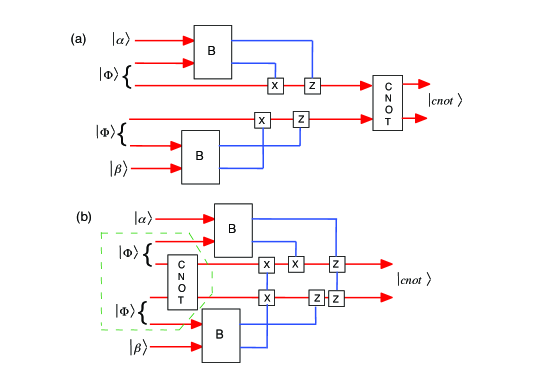
Figure 12: Schematic representation of gate operation via teleportation. Figures (a) and (b) are equivalent, yet in (b) a non-deterministic CNOT gate is sufficient as failure only destroys the entanglement: the operation can be repeated till successful without losing the qubit.

The simplest teleportation gate is shown in Fig.13. The heart of the gate is a teleported single-rail CS gate. CS operation on single-rail qubits can equally well be used to produce CS operation on dual-rail qubits simply by adding additional rails which do not participate in the interaction (Fig.13). The entangled resource is the state

$$|0101\rangle+|0110\rangle+|1001\rangle-|1010\rangle$$ (59)

which can be interpreted as two single rail Bell states which have had a CS gate applied between them in analogy with the resource state in Fig.12 (b). Alternatively one can recognize this state as the dual-rail Bell state $|0101\rangle+|1010\rangle$ with a Hadamard gate applied to the second qubit. Such a state can be generated directly by down conversion. This latter interpretation is due to Pittman, Jacobs and Franson PIT01 .

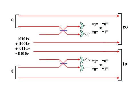
Figure 13: Schematic representation of optical CS gate operation via teleportation. Success is heralded by a single photon being detected at each of the two pairs of detectors. If zero (two) photons are detected at one of the detector pairs then the corresponding qubit has been measured to be in the zero (one) logical state and the gate has failed. The probability of success of the gate is 25%.

Single-rail partial Bell measurements are used, as described in section V. These fail 50% of the time thus the probability of success of this gate is 25%. Because the partial Bell measurements fail by measuring their inputs in the computational basis, so the teleportation gate fails in the same way by measuring the logical values of the input qubits. The key to scale up is that this failure mode can be encoded against, as will be described in the next section.

An in principle demonstration of this gate was made by Gasparoni et al GAS04 . A femto-second pump pulse was double passed through a down conversion crystal to produce two entangled pairs of photons, one of which was used as the entangled resource whilst the other pair served as the input qubits. Gate operation was demonstrated with an average gate fidelity that can be estimated to be about 78%. Other demonstrations of this type of gate have been made by Pittman et al PIT03 and Zhao et al ZHA04 . Although this gate is in principle heralded it is important to note that the current low efficiencies of the sources and detectors mean all experiments so far have relied on coincidence detection.

KLM showed that by using more complex entangled states teleportation gates with a higher probability of success could be implemented. Consider the entangled state

$$|0011\rangle+|1010\rangle+|1100\rangle.$$ (60)

If the first two modes of this entangled state are mixed with an input qubit on a beam tritter (i.e. an arrangement of beamsplitters that coherently mixes three input fields in equal ratios) and are then photon counted, teleportation can be achieved for certain measurement outcomes. For example if the measurement result is ”$100$”, then the conditional state of the remaining two modes of the entanglement will be $\alpha|10\rangle+\beta|11\rangle$. The state has been successfully teleported to the last mode. The other mode is definitely in the ”$1$” state and can be discarded. Similarly if the measurement result ”$200$” was recorded then the conditional state of the remaining two modes of the entanglement will be $\alpha|00\rangle+\beta|10\rangle$. Now the state has been successfully teleported to the first of the remaining modes, whilst the other mode is definitely in the ”$0$” state and can be discarded. Other measurement results will require phase shifts of $\pm\pi/\sqrt{3}$ to recover the qubit. If no photons are counted (assuming unit detection efficiency) or $3$ photons are counted then the original qubit must have been in the ”$0$” or ”$1$” states respectively and the teleportation fails by measurement of the qubit. The combined probability of these failure modes is $1/3$ so the teleporter has a $2/3$ probability of success.

This more efficient teleporter can then be used to implement a teleportation gate with a probability of success of $4/9$ using the entanglement resource

$$|00110011\rangle+|00111010\rangle+|00111100\rangle+|10100011\rangle$$

$$\;\;\;-|10101010\rangle+|10101100\rangle+|11000011\rangle$$

$$\;\;\;\;\;\;+|11001010\rangle+|11001100\rangle.$$ (61)

which is two entangled states of the form of Eq.60 with CS gates applied between all the possible combinations of output modes. This state could be produced non-deterministically using the level one gates but with considerable overhead. Higher order gates with even better probabilities of success are possible with correspondingly more complicated resource entanglement. Because of the high cost of producing the entanglement this is not a viable approach to scalability. Instead, in the next section, we discuss the much more promising approach of error encoding.

VI.2.3 Error Encoding Against Teleportation Failure

In the previous section we have seen that teleportation gates can be implemented which have higher probability of success than the first tier non-deterministic gates. A key feature of these gates is that failure results in the measurement of the logical values of the qubits. KLM introduced an error correction code to protect against such computational basis measurements (Z-measurements) of the qubits. A logical qubit can be encoded across 2 physical qubits as KNI01

$$|\phi\rangle^{(2)}=\alpha(|\bf 0\rangle|\bf 0\rangle+|\bf 1\rangle|\bf 1\rangle)+\beta(|\bf 0\rangle|\bf 1\rangle+|\bf 1\rangle|\bf 0\rangle)$$ (62)

This is a parity encoding, that is the “zero” state is represented by an equal superposition of all the even parity combinations of the 2 qubits whilst the “one” state is represented by all the odd parity combinations. Notice that if a Z-measurement is made on either of the physical qubits of the state in Eq.62 and the result “0” is obtained, then the state collapses to an unencoded qubit, however the superposition is preserved. Similarly if the measurement result is “1” a bit-flipped version of the unencoded qubit is the result, but again the superposition is preserved so the qubit can be recovered.

This encoding thus enables recovery from teleportation gate failure and so improves the probability of success of the gate by allowing second attempts. An in principle demonstration of this encoding was made by O’Brien et al OBR05 using the two photon CNOT gate discussed in section VI.2.1 to produce the required parity encoded states, where the CNOT gate takes an unencoded qubit as its target input and a diagonal state as its control input. It was shown that measurement of either physical qubit led to the expected unencoded qubit being projected onto the remaining photon to an accuracy of greater than 90% fidelity.

Notice that a two-qubit (and thus non-deterministic) gate is needed to produce the parity encoding. It is not immediately obvious that producing encoded states non-deterministically which then can be used to improve the performance of more non-deterministic gates, is a winning strategy. KLM showed however, that provided you start with teleporters with a probability of success greater than 50%, this strategy does improve gates success. For example a $2/3$ teleporter used with the parity encoding leads to a CS gate success probability of about 58% (as opposed to 44% without encoding). In order to further improve the probability of success KLM concatenates the two qubit parity code. For example the next level up logical qubit is given by

$$|\phi\rangle_{L4} = \alpha(|{\bf 0}\rangle^{(2)}|{\bf 0}\rangle^{(2)}+|{\bf 1}\rangle^{(2)}|{\bf 1}\rangle^{(2)})$$ (63)

$$\;\;\;\;\;\;\;\;+\beta(|{\bf 0}\rangle^{(2)}|{\bf 1}\rangle^{(2)}+|{\bf 1}\rangle^{(2)}|{\bf 0}\rangle^{(2)})$$

High probabilities of success are obtained after a few levels of concatenation, leading to the claim of a scalable system.

VI.2.4 Parity States and Cluster States

KLM was a major step forward both in opening the door to small-scale demonstrations of optical quantum circuits, and in pointing the way towards a scalable system. However, in its original form the resources required for scale-up were exorbitant. For example the number of Bell pairs needed to implement a single CS gate with 95% probability of success using the original KLM approach can be estimated to be in the 10,000’s. Fortunately, considerable progress has been made in recent years in reducing this overhead YOR03 ; NIE04 ; HAY04 with the most efficient approaches requiring of order 100 Bell pairs for a CS with $>95\%$ success BRO05 ; GIL05 . Two related but distinct approaches have emerged which we now discuss.

An alternative way to scale up the parity states, introduced by Hayes et al HAY04 , is not to concatenate the code as per Eq.63, but instead to increase it incrementally. Hence a logical qubit can be encoded across $n$ qubits by representing logical “zero” by all the even parity combinations of the $n$ qubits and logical “one” by all the odd parity combinations. This code retains the feature that if the logical qubit is encoded across $n$ physical qubits then a computational basis measurement on any one of the qubits reduces the state to a logical qubit encoded across $(n-1)$ physical qubits (with the possible need for a bit-flip). Specifically, this parity encoding is given by

$$|{\bf 0}\rangle^{(n)} \equiv (|+\rangle^{\otimes n}+|-\rangle^{\otimes n})/\sqrt{2}$$

$$|1\rangle^{n} \equiv (|+\rangle^{\otimes n}-|-\rangle^{\otimes n})/\sqrt{2},$$ (64)

where $|\pm\rangle=(|{\bf 0}\rangle\pm|{\bf 1}\rangle)/\sqrt{2}$.

There are two operations which are easily performed on parity encoded states: a rotation by an arbitrary amount around the $x$ axis of the Bloch sphere (i.e. $X_{\theta}=\cos(\theta/2)I+i\sin(\theta/2)X$) NOTE2 , which can be performed by applying that operation to any of the physical qubits and; a $Z$ operation, which can be performed by applying $Z$ to all the physical qubits (since the odd-parity states will acquire an overall phase flip).

The teleportation gates are reduced to just partial single-rail and dual-rail Bell-state measurements. A dual-rail Bell measurement can be used to add $n$ physical qubits to a parity encoded state using a resource of $|{\bf 0}\rangle^{(n+2)}$. This is referred to as type-II fusion ($f_{II}$) BRO05 . The result of $f_{II}$ is

$$f_{II}|\psi\rangle^{(m)}|{\bf 0}\rangle^{(n+2)}\rightarrow\left\{\begin{array}[]{cl}|\psi\rangle^{(m+n)}&\mbox{(success)}\\ |\psi\rangle^{(m-1)}|{\bf 0}\rangle^{(n+1)}&\mbox{(failure)}\end{array}\right.$$ (65)

When successful (with probability $1/2$), the length of the parity qubit is extended by $n$. A phase flip correction may be necessary depending on the outcome of the Bell-measurement. If unsuccessful a physical qubit is removed from the parity encoded state, and the resource state is left in the state $|{\bf 0}\rangle^{(n+1)}$ (which may be recycled). This encoding procedure is equivalent to a gambling game where we either lose one level of encoding, or gain $n$ depending on the toss of a coin. Clearly if $n\geq 2$ this is a winning game. The required resource states can be built from Bell pairs using a combination of single-rail Bell measurements (type I fusion) and $f_{II}$. The remaining gates in order to achieve a universal gate set (a $Z_{90}$ and a cnot gate) can be efficiently performed using these fusion techniques GIL05 . The resource overhead for performing gates in this way is of order 100 Bell pairs per gate.

Raussendorf and Briegel have suggested an alternative way of performing quantum computing, distinct from the usual circuit model, called cluster-state quantum computation RAU01 . It is based on measurement induced quantum evolution and so is sometimes referred to as ”one-way” quantum computation. In their approach a large entangled state of a particular form, called a cluster state, is constructed first. Quantum computation is then carried out by making a series of measurements on the cluster state. For example any evolution of a single qubit can be simulated by: (i) preparing a string of qubits all in the states $|\bf 0\rangle+|\bf 1\rangle$; (ii) linking each nearest neighbour by C-S gates (this forms a linear cluster state), and then; (iii) measuring the single qubits in the string in sequence. The measurement basis chosen for each qubit depends on the single qubit unitaries one wishes to simulate and the result of the measurement of the preceding qubit. Each qubit measurement simulates the unitary evolution $HZ_{\theta}$ where $H$ is the Hadamard transformation and $Z_{\theta}$ is a rotation about $z$. An arbitrary single qubit unitary can be simulated using a four qubit cluster state and three measurements.

We can illustrate this by considering an arbitrary rotation about $x$, $X_{\theta}=HZ_{\theta}H$ which can be achieved with a 3 qubit cluster state and 2 measurements. The first qubit is prepared in some arbitrary state $\alpha|\bf 0\rangle+\beta|\bf 1\rangle$. A cluster state is then formed by applying C-S gates to the arbitrary qubit and two other qubits prepared in diagonal states, resulting in the state $\alpha(|\bf 000\rangle+|\bf 010\rangle+|\bf 001\rangle-|\bf 011\rangle)+\beta(|\bf 100\rangle+|\bf 101\rangle-|\bf 110\rangle+|\bf 111\rangle)$. The idea is then to simulate the single qubit x rotation via measurement. The first qubit is measured in the diagonal basis: $|D1\rangle=|\bf 0\rangle+|\bf 1\rangle$, $|D2\rangle=-|\bf 0\rangle+|\bf 1\rangle$. If the outcome is $D1$ then the second qubit is measured in the phase rotated basis: $|R1(\theta)\rangle=|\bf 0\rangle+\exp{i\theta}|\bf 1\rangle$, $|R2(\theta)\rangle=-|\bf 0\rangle+\exp{i\theta}|\bf 1\rangle$. If, on the other hand, the outcome is $D2$ then the second qubit is measured in the phase anti-rotated basis: $|R1(\theta)\rangle=|\bf 0\rangle+\exp{-i\theta}|\bf 1\rangle$, $|R2(\theta)\rangle=-|\bf 0\rangle+\exp{-i\theta}|\bf 1\rangle$. After these measurements the state of the last qubit is the same as that of the original qubit, but rotated about x by an angle $\theta$. However the effective computational basis of the qubit depends on the outcomes of the measurements in the following way:
(i) $D1$, $R1(\theta)$: the original computational basis. (ii) $D1$, $R2(\theta)$: bit-flip of the original computational basis. (ii) $D2$, $R1(-\theta)$: phase-flip of the original computational basis. (ii) $D2$, $R2(-\theta)$: bit-flip and phase-flip of the original computational basis.

By joining linear chains with CS gates to create 2-dimensional cluster states, two qubit gates can be built into the cluster, enabling universal quantum computation. The first suggestion that measurement based quantum computation could help to reduce the resources in an optical system was made by Yoran and Resnik YOR03 . Subsequently Nielsen adapted the complete cluster state approach to LOQC NIE04 . He showed that cluster states could be efficiently built up using the teleportation gates. This follows from the fact that the cluster states are able to recover from computational basis measurements in a similar (but not identical) way to that of the parity states. The application of the fusion techniques described above BRO05 (which were in fact initially developed by Browne and Rudolph for cluster state production) further reduces the resource overhead. In this approach ”mini-cluster” states are built up non-deterministically and then fused on to the main cluster in a similar way to that already described for parity states. This is perhaps the most efficient of the photonic schemes, requiring approximately 60 Bell pairs per two-qubit gate, though the exact meaning of ”per gate” in the cluster state paradigm is more ambiguous than in circuit models such as the parity state approach.

In principle optical demonstrations of one-way quantum computation have now been achieved with coincidence counting. Simple cluster state computation using a 4 qubit cluster was demonstrated experimentally by Walther et al WAL05 . In this experiment the cluster state was generated directly from parametric down conversion. In other experiments the cluster states were constructed from Bell pairs by Zhang et al using the fusion technique ZHA05 and by Kiesel et al using the C-Sign gate KIE05 .

VI.2.5 Coherent States

Finally we note that a linear optics quantum computation scheme can also be constructed using the coherent state qubits discussed in section III. The basic resource state required is the superposition state: $|\alpha\rangle+|-\alpha\rangle$. These, in conjunction with homodyne detection, photon counting and linear optics, are sufficient to produce a scaleable system RMM ; RAL03 . As for the photonic approach the basic gates are non-deterministic and need to be scaled up by teleportation. Unlike the photonic approach the probability of success of the basic gates is much higher (80-90%) and (as we noted in section V) coherent state qubit teleportation is deterministic. This means that the over-heads for scale-up are much lower. On the other hand, the relative cost of the required superposition state resources compared to the Bell pairs needed for the photonic scheme are not known, making direct comparison’s difficult. A number of groups are currently working towards demonstrations of coherent state superpositions so these issues may become clearer soon.

VI.3 Fault Tolerance

When large scale quantum processing is considered we have to worry about the propagation of small errors inevitably introduced during gate operations. If uncorrected, such errors would grow uncontrollably and make the computation useless. The answer to this problem is fault tolerant error correction SHO95 ; STE96 . The idea of error correction is self-explanatory, though its implementation on quantum systems requires some care. Classically we might consider using a redundancy code such that (for example) $0\to 0,0,0$ and $1\to 1,1,1$. If a bit flip occurs on one of the bits we might end up with $0,1,0$ or $1,0,1$, but we can recover the original bit value by taking a majority vote. At first it may seem that such a code cannot be used for quantum mechanical systems because: (i) the no-cloning theorem WOO82 means we can not make copies of an unknown qubit and; (ii) taking the majority vote is a measurement that will collapse our quantum superposition. It turns out however that a quantum analog is possible. A quantum redundant encoding might be $\alpha|{\bf 0}\rangle+\beta|{\bf 1}\rangle\to\alpha|{\bf 000}\rangle+\beta|{\bf 111}\rangle$ where we have created an entangled state rather than copies. It is then possible, using two CNOT gates and two ancillas, to identify an error without collapsing the state, by reading out the parity of pairs of qubits. For example a bit-flip error might result in the state $\alpha|{\bf 001}\rangle+\beta|{\bf 110}\rangle$. The parity of the first two qubits will be zero whilst the parity of the second two qubits will be one, thus unambiguously identifying that an error has occured on the last qubit. Because we are measuring the parity, not the qubit value, the superposition is not collapsed. Such codes can be expanded to cope with the possibility of more than one error occurring between correction attempts and to cope with multiple types of errors. Of course the CNOT gates being used to detect and correct the errors may themselves be faulty. An error correction code is said to be fault tolerant if error propagation can be prevented even if the components used to do the error correction introduce errors themselves. Typically this is only possible if the error rate is below some level known as the fault tolerant threshold.

The original KLM paper KNI01 showed that in principle LOQC was fault tolerant, though a general threshold was not calculated. Optical cluster state computation has also been shown to be fault tolerant, with thresholds against depolarization errors of about a hundredth of a percent DAW05 . Although such a number is daunting, the precision of optics is such that it is not inconceivable. Presently the dominant error in optical quantum processing is loss, both in components, detectors and sources. The prospects for reducing loss to such levels are remote so some effort has gone into optimizing codes specifically against loss. KLM estimated a threshold of about 1% for loss tolerance (i.e. fault tolerance where the only error considered is loss). Remaining with the original KLM gate approach Silva et al were able to show that the loss threshold might lie as high as 11% SIL05 . Using the parity state approach and assuming that components, sources and detectors all had an equal loss of $x\%$, Ralph et al numerically obtained a loss threshold of $x=17\%$ RAL05 . A roughly equivalent value was obtained by Varnava et al for loss tolerance of cluster states VAR05 . These nice results for loss tolerance must be treated with some caution given the tougher figures for general fault tolerance, however it is encouraging that the most resource efficient approaches also seem to display good resilience.

VII Conclusion

Light holds a privileged position in quantum information science as the only reasonable candidate for quantum communication. This is not just because of its mobility, but also, as we have seen, because of the ease with which certain critical manipulations of quantum optical states can be achieved. The scope of quantum processing tasks that can be achieved in optics has expanded rapidly in recent years leading to remarkable progress in implementing quantum information protocols. The progress in QKD in particular is sufficiently advanced that commercial applications are seriously considered. Teleportation, of a quality clearly exceeding the limits set in the absence of entanglement, has been demonstrated in both the discrete and continuous domains. The demonstration of basic two-qubit quantum gates is promising but is a long way short of full-scale quantum computation. Continued advances along this path require technical solutions to the problem of efficient single photon production, detection and memory.

An exciting new direction that we have not discussed much here is the possibility of hybrid optical/atomic and/or solid-state systems. It has long been recognized that optical ”flying qubits” acting as a data bus can solve the connectivity problem in atomic or solid-state quantum computer architectures. Alternatively we might use the ”standing qubits” as memory, whilst processing the quantum information optically. The major problem with this idea has been the interface between the standing and flying qubits. Recently significant progress has been made in this direction. For example the ion trap photon source discussed in section III.4 KEL04 , being coherent, could in principle also act as an interface. Another possibility is to use optical quantum processing to entangle distant standing qubits, thus enabling teleportation of information between distant sites or the formation of cluster states for quantum computation KOK05 ; DUA05 . Recent experimental progress in this direction has included the demonstration of entanglement between ions and photons BLI04 . These and other emerging technologies combined with achievements described in this review indicate a bright future for quantum information processing in optics.

References

- (1) R.Landauer, Physics Today, 23 (May 1991).
- (2) M. Nielsen and I. Chuang, Quantum computation and quantum information (Cambridge University Press, Cambridge, UK 2000).
- (3) S.Wiesner, ACM Signact News, 15(1), 78 (1983).
- (4) C.H.Bennett and G.Brassard, Proceedings of IEEE International Conference on Computers, Systems and Signal Processing, Bangalore, India, p. 175 (1984).
- (5) W.K.Wootters and W.H.Zurek, Nature 299, 802 (1982).
- (6) C.H. Bennett, S.J.Wiesner, Phys.Rev.Lett. 69, 2881 (1992).
- (7) C.H.Bennett, G.Brassard, C.Crepeau, R.Jozsa, A.Peres, W.K.Wootters, Phys.Rev.Lett. 70, 1895 (1993).
- (8) R.P.Feynman, Foundations Phys. 16, 507 (1986).
- (9) D.Deutsch, Proc.Roy.Soc.London A400, 97 (1985).
- (10) P.W.Shor in Proceedings of the 35th Annual Symposium on the Foundations of Computer Science, 124-133 (IEEE Computer Society Press, Los Alamitos, California 1994).
- (11) P. Shor, Phys. Rev. A52, 2493-2496 (1995).
- (12) A. M. Steane, Phys. Rev. Lett. 77, 793-797 (1996).
- (13) L.K.Grover, Phys.Rev.Lett. 79, 325 (1997).
- (14) J.J.Sakuria, Modern Quantum Optics (Addison-Wesley, California 1985).
- (15) B.Schumacher, Phys.Rev.A 51, 2738 (1995).
- (16) Continuous Variable Quantum Information, Ed S.Braunstein and A.Pati, (Kluwer Academic Publishers, The Netherlands, 2003).
- (17) S.L.Braunstein and H.J.Kimble, Phys.Rev.Lett. 80, 869 (1998).
- (18) T.C.Ralph, Phys.Rev.A. 61, 010302(R) (2000).
- (19) M. Hillery, Phys. Rev. A61 022309 (2000).
- (20) D. Gottesman, A. Kitaev, J. Preskill, Phys Rev A 64, 012310 (2001).
- (21) T.C.Ralph, A.Gilchrist, G.J.Milburn, W.J.Munro and S.Glancy, Phys. Rev. A 68, 042319 (2003).
- (22) The Principles of Quantum Mechanics, 4th edition, P.A.M.Dirac, Oxford University Press, London (1958).
- (23) R.J.Glauber, Phys.Rev. 131, 2766(1962).
- (24) Quantum statistical properties of radiation, W.H.Louisell, Wiley, New York (1973).
- (25) H.J.Kimble, M.Dagenais, L.Mandel, Phys.Rev.Lett. 39, 691(1977).
- (26) H.J.Carmichael, D.F.Walls, J.Phys.B 9, 1199 (1976).
- (27) A.Aspect, P.Grangier, G.Roger, Phys.Rev.Lett. 47, 460 (1981).
- (28) Foundations of Quantum Mechanics, J.S.Bell, Ed.B.d’Espagnat, (New York: Academic) 171 (1971).
- (29) J.F.Clauser, M.A.Horne, A.Shimony and R.A.Holt, Phys.Rev.Lett. 23, 880 (1969).
- (30) S.J.Freedman and J.F.Clauser, Phys.Rev.Lett. 28, 938 (1972).
- (31) P.Grangier, G.Roger and A.Aspect, Europhys. Lett. 1, 173 (1986).
- (32) R.Ghosh and L.Mandel, Phys.Rev.Lett. 59, 1903 (1987).
- (33) C.K.Hong, Z.Y.Ou, L.Mandel, Phys.Rev.Lett. 59, 2044 (1987).
- (34) H.P.Yuen, Phys.Rev.A 13, 2226 (1976).
- (35) D.F.Walls, Nature 306, 141 (1983).
- (36) Ling-An Wu, Min Xiao, H.J.Kimble, J.Opt.Soc.Am.B 4, 1465 (1987).
- (37) A.Einstein, B.Podolsky, N.Rosen, Phys.Rev.47, 777 (1935).
- (38) Z.Y.Ou, S.F.Pereira, H.J.Kimble, K.C.Peng, Phys.Rev.Lett. 68, 3663 (1992).
- (39) K. Mølmer, Phys. Rev. A 55, 3195 (1997)
- (40) Y.Yamamoto, H.A.Haus, Rev.Mod.Phys. 58, 1001 (1986).
- (41) C.M.Caves and P.D.Drummond, Rev.Mod.Phys. 66, 481 (1994).
- (42) C.E.Shannon, Bell System Tech. J. 27, 623 (1948).
- (43) N.J.Cerf, S.Iblisdir and G.V.Assche, Eur. Phys. J. D 18, 211(2002).
- (44) H.P.Yuen, J.H.Shapiro, IEEE Trans.Inform.Theory Vol.IT-24, 657 (1978).
- (45) H-A.Bachor and T.C.Ralph, A guide to experiments in quantum optics (2nd Edition, Wiley-VCH, Weinheim 2004).
- (46) J. L. Dodd, T. C. Ralph, and G. J. Milburn, Phys. Rev. A 68, 042328 (2003).
- (47) D.Stucki, N.Gisin, O.Guinnard, G.Ribordy, H.Zbinden, New J.Phys. 4, 41 (2002).
- (48) E.H.Huntington and T.C.Ralph, Phys. Rev. A 69, 042318 (2004).
- (49) A. P. Lund, T. C. Ralph, Phys. Rev. A, 66, 032307 (2002).
- (50) A. I. Lvovsky and J. Mlynek Phys. Rev. Lett. 88, 250401 (2002).
- (51) S. A. Babichev, B. Brezger, and A. I. Lvovsky Phys. Rev. Lett. 92, 047903 (2004).
- (52) P. Cochrane, G. J. Milburn and W. J. Munro, Phys Rev A 59, 2631 (1998).
- (53) S. J. van Enk and O. Hirota, Phys. Rev. A64, 022313 (2001).
- (54) H. Jeong, M. S. Kim, and J. Lee Phys. Rev. A64, 052308 (2001).
- (55) M. Brune, E. Hagley, J. Dreyer, X. Maitre, A. Maali, C. Wunderlich, J. M. Raimond and S. Haroche, Phys Rev Lett 77, 4887 (1996).
- (56) Q. A. Turchette et al, C. J. Hood, W. Lange, H. Mabuchi and H. J.Kimble, Phys Rev Lett 75, 4710 (1995).
- (57) A.P.Lund, H.Jeong, T.C.Ralph and M.S.Kim, Phys.Rev.A (R) 70, 020101 (2004).
- (58) J. Wenger, R. Tualle-Brouri, and P. Grangier, 92, 153601 (2004).
- (59) A.I.Lvovsky, H.Hansen, T.Aichele, O.Benson, J.Mlynek, S.Schiller Phys.Rev.Lett. 87, 050402 (2001).
- (60) D. T. Smithey, M. Beck, M. G. Raymer, and A. Faridani Phys. Rev. Lett. 70, 1244 (1993).
- (61) C.Kurtsiefer, M.Oberparleiter, H.Weinfurter Phys.Rev. A 64, 023802 (2001).
- (62) A.Migdall, D.Branning and S.Casteletto, Phys. Rev. A 66, 053805 (2002).
- (63) T.B.Pittman, B.C.Jacobs, J.D.Franson, Phys.Rev. A 66, 042303 (2002).
- (64) A.Kuhn, G.Rempe, Phys.Rev.Lett. 89, 067901 (2002).
- (65) M.Keller, B.Lange, K.Hayasaka, W.Lange and H.Walther, Nature 431, 1075 (2004).
- (66) A.Beveratos, R.Brouri, T.Gacoin, A.Villing, J.-P.Poizat, P.Grangier, Phys.Rev.Lett. 89, 187901 (2002).
- (67) C.Santori, D.Fattal, J.Vuckovic, G.S.Solomon, Y.Yamamoto, Nature, 419, 594 (2002).
- (68) A.Kiraz, M.Atat re and A.Imamoglu,Phys.Rev. A 69, 032305 (2004).
- (69) G.G. Stokes, Trans. Cambridge Philos. Soc. 9, 399 (1852).
- (70) A.G.White, D.F.V.James, P.H.Eberhard, P.G.Kwiat, Phys.Rev.Lett. 83, 3103 (1999).
- (71) D.F.V.James, P.G.Kwiat, W.J.Munro, A.G.White, Phys.Rev. A 64, 052312 (2001)
- (72) J.L.O Brien, G.J.Pryde, A.Gilchrist, D.F.V.James, N.K.Langford, T.C.Ralph and A.G.White, Phys.Rev.Lett. 93, 080502 (2004).
- (73) C.H.Bennett, G.Brassard, C.Crepeau, U.M.Maurer, IEEE Trans. Inf. Theory 41, 1915 (1995).
- (74) D.Gottesman, H.-K.Lo, IEEE Transactions on Information Theory 49, 457 (2003).
- (75) C.H.Bennett, F.Bessette, G.Brassard, L.Salvail, J.Smolin, J.Cryptol 5, 3 (1992).
- (76) R.J.Hughes, J.E.Nordholt, D.Derkacs, C.G.Peterson, New J.Phys. 4, 43 (2002).
- (77) N.Gisin, G.Ribordy, W.Tittel, and H.Zbinden, Rev. Mod. Phys. 74, 145 (2002).
- (78) F.Grosshans, P.Grangier, Phys.Rev.Lett. 88, 057902 (2002).
- (79) Ch.Silberhorn, T.C.Ralph, N.Lutkenhaus and G.Leuchs, Phys.Rev.Lett. 89, 167901 (2002).
- (80) C.Weedbrook, A.M.Lance, W.P.Bowen, T.Symul, T.C.Ralph, P.K.Lam, Phys. Rev. Lett. 93, 170504 (2004).
- (81) F.Grosshans Phys. Rev. Lett. 94, 020504 (2005).
- (82) D.Gottesman, J.Preskill, Phys.Rev. A 63, 022309 (2001).
- (83) F.Grosshans, G.V.Assche, J.Wenger, R.Brouri, N.J.Cerf, P.Grangier, Nature, 421, 238 (2003).
- (84) S.Lorenz, N.Korolkova, G.Leuchs, Appl. Phys. B 79, 273 (2004).
- (85) A.M.Lance, T.Symul, V.Sharma, C.Weedbrook, T.C.Ralph, and P.K.Lam, Phys. Rev. Lett. 95, 180503 (2005).
- (86) C. H. Bennett and S. J. Wiesner, Phys.Rev.Lett. 69, 2881 (1992).
- (87) S. L. Braunstein and H. J. Kimble, Phys.Rev.A 61, 042302 (2000).
- (88) T.C.Ralph and E.H.Huntington, Phys.Rev.A 66, 042321 (2002).
- (89) K. Mattle, H. Weinfurter, P. G. Kwiat and A. Zeilinger, Phys.Rev.Lett. 76, 4656 (1996).
- (90) X. Li, Q. Pan, J. Jing, J. Zhang, C. Xie and K. Peng, Phys.Rev.Lett. 88, 047904 (2002).
- (91) R. Cleve, D. Gottesman, and H.-K. Lo, Phys. Rev. Lett. 83, 648 (1999).
- (92) T. Tyc, D. J. Rowe, and B. C. Sanders, J. Phys. A 36, 7625 (2003).
- (93) A. M. Lance, T. Symul, W. P. Bowen, B. C. Sanders, and P. K. Lam, Phys. Rev. Lett. 92, 177903 (2004).
- (94) P.G.Kwiat, K.Mattle, H.Weinfurter, A.Zeilinger, A.V.Sergienko, Y.Shih, Phys.Rev.Lett. 75, 4337 (1995).
- (95) H. Weinfurter, Europhys. Lett. 25, 559 (1994).
- (96) S. L. Braunstein and A. Mann, Phys. Rev. A 51, R1727 (1995).
- (97) D.Bouwmeester, J.-W.Pan, K.Mattle, M.Eibl, H.Weinfurter, A.Zeilinger, Nature 309, 575 (1997).
- (98) J.-W.Pan, S.Gasparoni, M.Aspelmeyer, T.Jennewein, A. Zeilinger, Nature 421, 721 (2003).
- (99) E.Lombardi, F.Sciarrino, S.Popescu, and F. De Martini Phys. Rev. Lett. 88, 070402 (2002).
- (100) L.Vaidman, Phys.Rev.A 49, 1473 (1994).
- (101) M.D.Reid, P.D.Drummond, Phys.Rev.Lett. 60, 2731 (1988).
- (102) A.Furusawa, J.L.Sörensen, S.L.Braunstein, C.A.Fuchs, H.J.Kimble, E.S.Polzik, Science, 282, 706 (1998).
- (103) W.P.Bowen, N.Treps, B.C.Buchler, R.Schnabel, T.C.Ralph, H-A.Bachor, T.Symul, P.K.Lam, Phys. Rev. A 67, 032302 (2003).
- (104) T.C.Ralph and P.K.Lam, Phys.Rev.Lett. 81, 5668 (1998).
- (105) E.Arthurs, M.S.Goodman, Phys.Rev.Lett. 60, 2447 (1988).
- (106) T.C.Ralph, P.K.Lam and R.E.S.Polkinghorne, Journal Of Optics B, 1, 483 (1999).
- (107) F.Grosshans, P.Grangier, Phys.Rev. A 64, 010301 (2001).
- (108) C.M.Caves and K.W dkiewicz Phys. Rev. Lett. 93, 040506 (2004).
- (109) N.Takei, H.Yonezawa, T.Aoki and A.Furusawa, Phys. Rev. Lett. 94, 220502 (2005).
- (110) G.J.Milburn, Phys.Rev.Lett. 62, 2124 (1989).
- (111) L.-M. Duan and H. J. Kimble Phys. Rev. Lett. 92, 127902 (2004).
- (112) K.Nemoto and W.J.Munro Phys. Rev. Lett. 93, 250502 (2004).
- (113) E.Knill, R.Laflamme, G.J.Milburn, Nature 409, 46 (2001).
- (114) M.Reck, A.Zeilinger, H.J.Bernstein and P.Bertani, Phys. Rev. Lett. 73, 58(1994).
- (115) P.G.Kwiat, J.R.Mitchell, P.D.D.Schwindt, A.G.White, J.Mod.Opt. 47, 257(2000).
- (116) N.Bhattacharya H.B.van Linden van den Heuvell and R.J.C.Spreeuw, Phys. Rev. Lett. 88, 137901 (2002).
- (117) S.Lloyd Phys. Rev. A 61, 010301 (2000)
- (118) In fact it was reported very recently that the experiment has now been repeated at the single photon level: O.Hosten, et al, QELS presentation QTuJ6, Baltimore (2005).
- (119) T.C.Ralph, A.G.White, W.J.Munro, G.J.Milburn, Phys.Rev. A 65, 012314 (2002).
- (120) J.Eisert, Phys. Rev. Lett. 95, 040502 (2005).
- (121) T.C.Ralph, N.K.Langford, T.B.Bell, A.G.White, Phys.Rev. A 65, 062324 (2002).
- (122) H.F.Hofmann and S.Takeuchi Phys. Rev. A 66, 024308 (2002)
- (123) J.L.O’Brien, G.J.Pryde, A.G.White, T.C.Ralph, D.Branning, Nature 426, 264(2003).
- (124) J.L.O Brien, G.J.Pryde, A.Gilchrist, D.F.V.James, N.K.Langford, T.C.Ralph and A.G.White, Phys.Rev.Lett. 93, 080502 (2004).
- (125) D.Gottesman, I.L.Chuang, Nature 402, 390 (1999).
- (126) T.B.Pittman, B.C.Jacobs, and J.D.Franson, Phys. Rev. A 64, 062311 (2001).
- (127) S.Gasparoni, J.-W.Pan, P.Walther, T.Rudolph, and A.Zeilinger Phys. Rev. Lett. 93, 020504 (2004).
- (128) T.B.Pittman, M.J.Fitch, B.C.Jacobs, and J.D.Franson, Phys. Rev. A 68, 032316 (2003).
- (129) Z.Zhao, A.-N.Zhang, Y.-A.Chen, H.Zhang, J.-F.Du, T.Yang, and J.-W.Pan, Phys. Rev. Lett. 94, 030501 (2005).
- (130) J.L.O’Brien, G.J.Pryde, A.G.White, T.C.Ralph, Phys. Rev. A 71, 060303 (2005).
- (131) N.Yoran and B.Reznik, Phys. Rev. Lett. 91, 037903 (2003).
- (132) M.Nielsen, Phys. Rev. Lett. 93, 040503 (2004).
- (133) A.J.F.Hayes, A.Gilchrist, C.R.Myers and T.C.Ralph, J.Opt.B 6, 533 (2004).
- (134) D.E.Browne and T.Rudolph, Phys. Rev. Lett. 95, 010501 (2005).
- (135) A.Gilchrist, A.J.F.Hayes and T.C.Ralph, quant-ph/0505125.
- (136) , , and are the usual Pauli operators defined in Section V and an angle subscript denotes a rotation about that axis, analogous to defined in the text.
- (137) R.Raussendorf and H.J.Briegel, Phys.Rev.Lett. 86, 5188 (2001).
- (138) P.Walther, K.J.Resch, T.Rudolph, E.Schenck, H.Weinfurter, V.Vedral, M.Aspelmeyer, A.Zeilinger, Nature 434, 169(2005).
- (139) An-Ning Zhang, Chao-Yang Lu, Xiao-Qi Zhou, Yu-Ao Chen, Zhi Zhao, Tao Yang, Jian-Wei Pan, quant-ph/0501036.
- (140) N.Kiesel, C.Schmid, U.Weber, O.Guehne, G.Toth, R.Ursin, H.Weinfurter, quant-ph/0508128.
- (141) T. C. Ralph, W. J. Munro and G. J. Milburn, Proceedings of SPIE 4917, 1 (2002); quant-ph/0110115.
- (142) C.M.Dawson, H.L.Haselgrove, M.A.Nielsen, quant-ph/0509060.
- (143) M.Silva, M.Roetteler, C.Zalka, quant-ph/0502101.
- (144) T.C.Ralph, A.J.F.Hayes and A.Gilchrist, Phys. Rev. Lett. 95, 100501 (2005).
- (145) M.Varnava, D.E.Browne and T.Rudolph, quant-ph/0507036.
- (146) S.D.Barrett and P.Kok, Phys. Rev. A 71, 060310 (2005).
- (147) L.-M. Duan and R. Raussendorf, Phys. Rev. Lett. 95, 080503 (2005).
- (148) B.B.Blinov, D.L.Moehring, L.- M.Duan and C.Monroe, Nature 428, 153 (2004).