Optimal Control for Generating Quantum Gates in Open Dissipative Systems

Zusammenfassung

Optimal control methods for implementing quantum modules with least amount of relaxative loss are devised to give best approximations to unitary gates under relaxation. The potential gain by optimal control using relaxation parameters against time-optimal control is explored and exemplified in numerical and in algebraic terms: it is the method of choice to govern quantum systems within subspaces of weak relaxation whenever the drift Hamiltonian would otherwise drive the system through fast decaying modes. In a standard model system generalising decoherence-free subspaces to more realistic scenarios, opengrape-derived controls realise a cnot with fidelities beyond $95$% instead of at most $15\%$ for a standard Trotter expansion. As additional benefit it requires control fields orders of magnitude lower than the bang-bang decouplings in the latter.

I Introduction

Using experimentally controllable quantum systems to perform computational tasks or to simulate other quantum systems Feynman (1982, 1996) is promising: by exploiting quantum coherences, the complexity of a problem may reduce when changing the setting from classical to quantum. Protecting quantum systems against relaxation is therefore tantamount to using coherent superpositions as a resource. To this end, decoherence-free subspaces have been applied Zanardi and Rasetti (1998), bang-bang controls Viola et al. (2000) have been used for decoupling the system from dissipative interaction with the environment, while a quantum Zeno approach Misra and Sudarshan (1977) may be taken to projectively keep the system within the desired subspace Facchi and Pascazio (2001). Controlling relaxation is both important and demanding Viola and Lloyd (2001); Lidar and Whaley (2003); Facchi et al. (2005); Cappellaro et al. (2006), also in view of fault-tolerant quantum computing Kempe et al. (2001) or dynamic error correction Khodjasteh and Viola (2008). Implementing quantum gates or quantum modules experimentally is in fact a challenge: one has to fight relaxation while simultaneously steering the quantum system with all its basis states into a linear image of maximal overlap with the target gate. — Recently, we showed how near time-optimal control by grape Khaneja et al. (2005) take pioneering realisations from their fidelity-limit to the decoherence-limit Spörl et al. (2007).

In spectroscopy, optimal control helps to keep the state in slowly relaxing modes of the Liouville space Khaneja et al. (2003); Xu et al. (2004); Jirari and Pötz (2006). In quantum computing, however, the entire basis has to be transformed. For generic relaxation scenarios, this precludes simple adaptation to the entire Liouville space: the gain of going along protected dimensions is outweighed by losses in the orthocomplement. Yet embedding logical qubits as decoherence-protected subsystem into a larger Liouville space of the encoding physical system raises questions: is the target module reachable within the protected subspace by admissible controls?

In this category of setting, the extended gradient algorithm opengrape turns out to be particularly powerful to give best approximations to unitary target gates in relaxative quantum systems thus extending the toolbox of quantum control, see e.g. Lloyd (2000); Palao and Kosloff (2002); García-Ripoll et al. (2003); Ohtsuki et al. (2004); Khaneja et al. (2005); Schulte-Herbrüggen et al. (2005); Ganesan and Tarn (2005); Sklarz and Tannor (2006); Möttönen et al. (2006); D’Alessandro (2008). Moreover, building upon a precursor of this work Schulte-Herbrüggen et al. (2006), it has been shown in Rebentrost et al. (2009) that non-Markovian relaxation models can be treated likewise, provided there is a finite-dimensional embedding such that the embedded system itself ultimately interacts with the environment in a Markovian way. Time dependent $\Gamma(t)$ have recently also been treated in the Markovian Grace et al. (2007); Wu et al. (2007) and non-Markovian regime Gordon et al. (2008).

Here we study model systems that are fully controllable Sussmann and Jurdjevic (1972); Boothby and Wilson (1979); Schulte-Herbrüggen (1998); Altafini (2003), i.e. those in which—neglecting relaxation for the moment—to any initial density operator $\rho$, the entire unitary orbit $\mathcal{U}(\rho):=\{U\rho\,U^{-1}\,|\,U\;{\rm unitary}\}$ can be reached Albertini and D’Alessandro (2003) by evolutions under the system Hamiltonian (drift) and the experimentally admissible controls. Moreover, certain tasks can be performed within a subspace, e.g. a subspace protected totally or partially against relaxation explicitly given in the equation of motion.

II Theory

Unitary modules for quantum computation require synthesising a simultaneous linear image of all the basis states spanning the Hilbert space or subspace on which the gates shall act. It thus generalises the spectroscopic task to transfer the state of a system from a given initial one into maximal overlap with a desired target state.

II.1 Preliminaries

The control problem of maximising this overlap subject to the dynamics being governed by an equation of motion may be addressed by our algorithm grape Khaneja et al. (2005). For state-to-state transfer in spectroscopy, one simply refers to the Hamiltonian equations of motion known as Schrödinger’s equation (for pure states of closed systems represented in Hilbert space) or to Liouville’s equation (for density operators in Liouville space)

$$\dot{|\psi\rangle{}} = -iH\;|\psi\rangle{}$$ (1)

$$\dot{\rho} = -i\,[H,\rho]\;.$$ (2)

In quantum computation, however, the above have to be lifted to the corresponding operator equations, which is facilitated using the notations $\operatorname{Ad}_{U}(\cdot):=U(\cdot)U^{\dagger}$ and $\operatorname{ad}_{H}\,(\cdot):=[H,(\cdot)]$ with $U:=e^{-itH}$ obeying

$$e^{-it\operatorname{ad}_{H}}(\cdot)=\operatorname{Ad}_{U}(\cdot)$$ (3)

and using ‘$\circ$’ for the composition of maps in

$$\dot{U} = -iH\;U$$ (4)

$$\tfrac{\rm d}{{\rm d}t}\,{\rm Ad}_{U} = -i\operatorname{ad}_{H}\;\circ\;\operatorname{Ad}_{U}\;.$$ (5)

These operator equations of motion occur in two scenarios for realising quantum gates or modules $U(T)$ with maximum trace fidelities: The normalised quality function (setting $N:=2^{n}$ for an $n$-qubit system henceforth)

$$f^{\prime}:=\tfrac{1}{N}\,\operatorname{Re}\operatorname{tr}\{U_{\rm target}^{\dagger}U(T)\}$$ (6)

covers the case where overall global phases shall be respected, whereas if a global phase is immaterial Schulte-Herbrüggen et al. (2005) (while the fixed phase relation between the matrix columns is kept as opposed to ref. Tesch and de Vivie-Riedle (2004)), the quality function

$$f:=\tfrac{1}{N}\,\operatorname{Re}\operatorname{tr}\{\operatorname{Ad}_{U_{\rm target}}^{\dagger}\operatorname{Ad}_{U(T)}^{\phantom{\dagger}}\}=\big{|}f^{\prime}\big{|}^{2}$$ (7)

applies. The latter identity is most easily seen Schulte-Herbrüggen et al. (2005) in the so-called $vec$-representation Horn and Johnson (1991) of $\rho$ where one gets the conjugation superoperator $\operatorname{Ad}_{U}=\bar{U}\otimes U$ (with $\bar{U}$ denoting the complex conjugate) and the commutator superoperator $\operatorname{ad}_{H}={\rm 1\negthickspace l}{}\otimes H-H^{t}\otimes{\rm 1\negthickspace l}{}$.

II.2 Open grape

Likewise, under relaxation introduced by the operator $\Gamma$ (which may, e.g., take GKS-Lindblad form), the respective Master equations for state transfer Altafini (2003) and its lift for gate synthesis read

$$\dot{\rho} = -(i\operatorname{ad}_{H}\,+\,\Gamma)\;\rho$$ (8)

$$\dot{F} = -(i\operatorname{ad}_{H}\,+\,\Gamma)\;\circ\;F\quad.$$ (9)

Again with $N:=2^{n}$ in $n$-qubit system, $F$ denotes a quantum map in $GL(N^{2})$ as linear image over all basis states of the Liouville space representing the open system. The Lie-semigroup properties of $F(t)$ have recently been elucidated in detail Dirr et al. (2008): it is important to note that only in the special (and highly unusual) case of $[\operatorname{ad}_{H}\,,\,\Gamma\,]=0$ the map $F(t)$ boils down to a mere contraction of the unitary conjugation $\operatorname{Ad}_{U}$. In general, however, one is faced with an intricate interplay of the respective coherent ($i\operatorname{ad}_{H}$) and incoherent ($\Gamma$) part of the time evolution: it explores a much richer set of quantum maps than contractions of $\operatorname{Ad}_{U}$, as expressed in Dirr et al. (2008) in terms of a $\mathfrak{k},\mathfrak{p}$-decomposition of the generators in $\mathfrak{gl}(N^{2},\mathbb{C})$ of quantum maps. As will be shown below, it is this interplay that ultimately entails the need for relaxation-optimised control based on the full knowledge of the Master Eqn. (9), while in the special case of mere contractions of $\operatorname{Ad}_{U}$, tracking maximum qualities against fixed final times (‘top curves’, vide infra, e.g. Fig. 3 (a) upper panel) obtained for $\Gamma=0$ plus an estimate on the eigenvalues of $\Gamma$ suffice to come up with good guesses of controls.

$$\begin{CD}{\rho_{0}=\rho_{SE}(0)\otimes\rho_{B}(0)}@>{\quad\operatorname{Ad}_{W}(t)\quad}>{}>{\rho(t)=W(t)\rho_{0}W^{\dagger}(t)}\\ @V{\Pi_{SE}}V{\operatorname{tr}_{B}}V@V{\Pi_{SE}}V{\operatorname{tr}_{B}}V\\ {\rho_{SE}(0)}@>{\quad\;F_{SE}(t)\quad\;}>{}>{\rho_{SE}(t)}\\ @V{\Pi_{S}}V{\operatorname{tr}_{E}}V@V{\Pi_{S}}V{\operatorname{tr}_{E}}V\\ {\rho_{S}(0)}@>{\quad\;\,F_{S}(t)\quad\;\,}>{}>{\rho_{S}(t)}\end{CD}$$

Abbildung 1: Time-evolution of a quantum system ($S$) embedded in some environment ($E$) and coupled to a bath ($B$). If the universal system evolves under the global unitary $W(t)$, opengrape provides optimal controls for the category of scenarios for which there is a finite-dimensional embedding such that the embedded system ($SE$) follows a time evolution under a Markovian quantum map $F_{SE}(t)$, while the reduced system of concern ($S$) may evolve in a non-Markovian way by a generic quantum map $F_{S}(t)$. In the simplest of cases, $\rho_{SE}(0)$ is of tensor product form with $F_{S}(t)$ being Markovian itself.

Now for a Markovian Master equation to make sense in terms of physics, it is important that the quantum subsystem of concern is itself coupled to its environment in a way justifying to neglect any memory effects. This means the characteristic time scales under which the environment correlation functions decay have to be sufficiently smaller than the time scale for the quantum evolution of the subsystem (see, e.g., Breuer and Petruccione (2002)). — More precisely, as exemplified in Fig. 1, we will assume that either the quantum system itself ($S$) or a finite-dimensional embedding of the system ($SE$) can be separated from the environmental bath ($B$) such that (at least) one of the quantum maps of the reduced system $F_{S}(t)$ or $F_{SE}(t)$ is Markovian and allows for a description by a completely positive semigroup Gorini et al. (1976); Lindblad (1976); Davies (1976), if the time evolution for the universal composite of (embedded) system plus bath is unitary. Examples where $F_{S}(t)$ is Markovian have been given in a precursor Schulte-Herbrüggen et al. (2006) to this study, while a concrete setting of a qubit ($S$) coupled on a non-Markovian scale to a two-level fluctuator ($E$), which in turn interacts in a Markovian way with a bosonic bath ($B$) has been described in detail in Rebentrost et al. (2009).

Henceforth, for describing the method we will drop the subscript to the quantum map $F(t)$ and tacitly assume we refer to the smallest embedding such that the map is Markovian and governed by Eqn. (9).

Moreover, if the Hamiltonian is composed of the drift term $H_{d}$ and control terms $H_{j}$ with piecewise constant control amplitudes $u_{j}(t_{k})$ for $t_{k}\in[0,T]$

$$H(t_{k}):=H_{d}+\sum_{j}u_{j}(t_{k})H_{j}\quad\text{with}\;u_{j}(t_{k})\in\mathcal{U}\subseteq\mathbb{R}$$ (10)

then Eqn. (9) defines a bilinear control system.

With these stipulations, the grape algorithm can be lifted to the superoperator level in order to cope with open systems by numerically optimising the trace fidelity

$$f_{\rm tr}:=\operatorname{Re}\,\operatorname{tr}\{\operatorname{Ad}_{U_{\rm target}}^{\dagger}F(T)\}$$ (11)

for fixed final time $T$. For simplicity, we henceforth assume equal time spacing $\Delta t:=t_{k}-t_{k-1}$ for all time slots $k=1,2,\dots,M$, so $T=M\cdot\Delta t$. Therefore $F(T)=F_{M}\cdot F_{M-1}\cdots F_{k}\cdots F_{2}\cdot F_{1}$ with every map taking the form $F_{k}=\exp\{-(i\operatorname{ad}_{H(t_{k})}+\Gamma(t_{k}))\Delta t\}$ leads to the derivatives

$$\begin{split}\tfrac{\partial f_{\rm tr}}{\partial u_{j}(t_{k})}&=-\operatorname{Re}\ \operatorname{tr}\big{\{}\operatorname{Ad}^{\dagger}_{U}\cdot F_{M}\cdot F_{M-1}\cdots F_{k+1}\;\times\\ &\times\big{(}i\operatorname{ad}_{H_{j}}+\;\tfrac{\partial\Gamma(u_{j}(t_{k}))}{\partial u_{j}(t_{k})}\big{)}F_{k}\Delta t\times F_{k-1}\cdots F_{2}\cdot F_{1}\big{\}}\end{split}$$ (12)

for the recursive gradient scheme

$$u_{j}^{(r+1)}(t_{k})=u_{j}^{(r)}(t_{k})+\alpha_{r}\tfrac{\partial f_{\rm tr}}{\partial u_{j}(t_{k})}\quad,$$ (13)

where often the uniform $\Delta t$ is absorbed into the step size $\alpha_{r}>0$. It gives the update from iteration $r$ to $r+1$ of the control amplitude $u_{j}$ to control $H_{j}$ in time slot $t_{k}$.

Numerical Setting

Numerical opengrape typically started from some $50$ initial conditions to each fixed final time taking then some $r=10-30\times 10^{3}$ iterations (see Eqn. 13) to arrive at one point in the top curve shown as upper trace in Fig. 3.

In contrast, for finding time-optimised controls in the closed reference system, we used grape for tracking top curves: this is done by performing optimisations with fixed final time, which is then successively decreased so as to give a top curve $g(T)$ of quality against duration of control, a standard procedure used in, e.g., Ref. Schulte-Herbrüggen et al. (2005). Finding controls for each fixed final time was typically starting out from some $20$ random initial control sequences. Convergence to one of the points in time (where Fig. 3 shows mean and extremes for a familiy of $15$ different such optimised control sequences) required some $r=1000$ recursive iterations each. — Numerical experiments were carried out on single workstations with $512$ MHz to $1.2$ GHz tact rates and 512 MB RAM.

Clearly, there is no guarantee of finding the global optimum this way, yet the improvements are substantial.

III Exploring Applications by Model Systems

By way of example, the purpose of this section is to demonstrate the power of optimal control of open quantum systems as a realistic means for protecting from relaxation. In order to compare the results with idealised scenarios of ‘decoherence-free subspaces’ and ‘bang-bang decoupling’, we choose two model systems that can partially be tracted by algebraic means. Comparing numerical results with analytical ones will thus elucidate the pros of numerical optimal control over previous approaches. — In order to avoid misunderstandings, however, we should emphasize our algorithmic approach to controlling open systems (opengrape) is by no means limited to operating within such predesigned subspaces of weak decoherence: e.g., in Ref. Rebentrost et al. (2009) we have worked in the full Liouville space of a non-Markovian target system. Yet, not only are subspaces of weak decoherence practically important, they also lend themselves to demonstrate the advantages of relaxation-optimised control in the case of Markovian systems with time independent relaxation operator $\Gamma$, which we focus on in this section.

The starting point is the usual encoding of one logical qubit in Bell states of two physical ones

$$\begin{split}{|0\rangle{}}_{L}&:=\tfrac{1}{\sqrt{2}}\{|01\rangle{}+|10\rangle{}\}=|\psi^{+}\rangle{}\\ {|1\rangle{}}_{L}&:=\tfrac{1}{\sqrt{2}}\{|01\rangle{}-|10\rangle{}\}=|\psi^{-}\rangle{}\end{split}$$ (14)

Four elements then span a Hermitian operator subspace protected against $T_{2}$-type relaxation

$$\mathcal{B}:={\rm span}_{\mathbb{R}}\,\{|\psi^{\pm}\rangle\langle\psi^{\pm}|{}\}\quad.$$ (15)

This can readily be seen, since for any $\rho\in\mathcal{B}$

$$\Gamma_{0}(\rho):=[zz,[zz,\rho]]=0\quad,$$ (16)

where henceforth we use the short-hand $zz:=\sigma_{z}\otimes\sigma_{z}/2$ and likewise $xx$ as well as ${\rm 1\negthickspace l}{}\mu\nu{\rm 1\negthickspace l}{}:=\tfrac{1}{2}{\rm 1\negthickspace l}{}_{2}\otimes\sigma_{\mu}\otimes\sigma_{\nu}\otimes{\rm 1\negthickspace l}{}_{2}$ for $\mu,\nu\in\{x,y,z,{\rm 1\negthickspace l}{}\}$. Interpreting Eqn. 16 as perfect protection against $T_{2}$-type decoherence is in line with the slow-tumbling limit of the Bloch-Redfield relaxation by the spin tensor $A_{2,(0,0)}:=\tfrac{1}{\sqrt{6}}(\tfrac{3}{2}\,zz-\mathbf{I}_{1}\mathbf{I}_{2})$ Ernst et al. (1987)

$$\Gamma_{T_{2}}(\rho):=[A_{2,(0,0)}^{\dagger},[A_{2,(0,0)}^{\phantom{\dagger}},\rho]]=\tfrac{9}{24}[zz,[zz,\rho]]=0\;.$$ (17)

For the sake of being more realistic, the model relaxation superoperator mimicking dipole-dipole relaxation within the two spin pairs in the sense of Bloch-Redfield theory is extended from covering solely $T_{2}$-type decoherence to mildly including $T_{1}$ dissipation by taking (for each basis state $\rho$) the sum Ernst et al. (1987)

$$\Gamma(\rho)\;:=\sum\limits_{m_{1},m_{2}=-1}^{1}\big{[}A_{2,(m_{1},m_{2})}^{\dagger}\,,\,\big{[}A_{2,(m_{1},m_{2})}^{\phantom{\dagger}}\,,\,\rho\big{]}\big{]}\;,$$ (18)

in which the zeroth-order tensor $A_{2,(0,0)}\sim zz$ is then scaled 100 times stronger than the new terms. So the resulting model relaxation rate constants finally become $T_{2}^{-1}:T_{1}^{-1}=4.027$ s${}^{-1}:0.024$ s${}^{-1}\simeq 170\;:\;1$.

III.1 Controllability Combined with Protectability against Relaxation

In practical applications of a given system, a central problem boils down to simultaneously solving two questions: (i) is the (sub)system fully controllable and (ii) can the (sub)system be decoupled from fast relaxing modes while being steered to the target.

It is for answering these questions in algebraic terms that we have chosen the following coupling interactions: if the two physical qubits are coupled by a Heisenberg-XX interaction and the controls take the form of $z$-pulses acting jointly on the two qubits with opposite sign, one obtains the usual fully controllable logical single qubit over $\mathcal{B}$, because

$${\langle(z{\rm 1\negthickspace l}{}-{\rm 1\negthickspace l}{}z),(xx+yy)\rangle}_{\rm Lie}\overset{\rm rep}{=}\mathfrak{su}(2)\quad,$$ (19)

where ${\langle\cdot\rangle}_{\rm Lie}$ denotes the Lie closure under commutation (which here gives $(yx-xy)$ as third generator to $\mathfrak{su}(2)$).

Model System I

By coupling two of the above qubit pairs with an Ising-ZZ interaction as in Refs. Lidar and Wu (2002); Wu and Lidar (2002); Zanardi and Lloyd (2004) one gets the standard logical two-spin system serving as our reference System I: it is defined by the drift Hamiltonian $H_{D1}$ and the control Hamiltonians $H_{C1},H_{C2}$

$$\begin{split}H_{D1}:=&J_{xx}\;(xx{\rm 1\negthickspace l}{}{\rm 1\negthickspace l}{}+{\rm 1\negthickspace l}{}{\rm 1\negthickspace l}{}xx+yy{\rm 1\negthickspace l}{}{\rm 1\negthickspace l}{}+{\rm 1\negthickspace l}{}{\rm 1\negthickspace l}{}yy)+J_{zz}\,{\rm 1\negthickspace l}{}zz{\rm 1\negthickspace l}{}\qquad\\ H_{C1}:=&z{\rm 1\negthickspace l}{}{\rm 1\negthickspace l}{}{\rm 1\negthickspace l}{}-{\rm 1\negthickspace l}{}z{\rm 1\negthickspace l}{}{\rm 1\negthickspace l}{}\\ H_{C2}:=&{\rm 1\negthickspace l}{}{\rm 1\negthickspace l}{}z{\rm 1\negthickspace l}{}-{\rm 1\negthickspace l}{}{\rm 1\negthickspace l}{}{\rm 1\negthickspace l}{}z\;,\\[-14.22636pt] \end{split}$$ (20)

where the coupling constants are set to $J_{xx}=2$ Hz and $J_{zz}=1$ Hz. Hence, over the $T_{2}$-decoherence protected subspace spanned by the four-qubit Bell basis $\mathcal{B}\otimes\mathcal{B}$ one obtains a fully controllable logical two-qubit system

$${\langle{H_{D1}},{H_{C1}},{H_{C2}}\rangle}_{\rm Lie}\,\big{|}_{\mathcal{B}\otimes\mathcal{B}}\overset{\rm rep}{=}\mathfrak{su}(4)\quad.$$ (21)

As illustrated in Fig. 2, in the eigenbasis of $\Gamma$ (of Eqn. 18) the Hamiltonian superoperators $\operatorname{ad}_{H}$ take block diagonal form, where the first block acts on the Liouville subspace $\mathcal{B}\otimes\mathcal{B}$ spanning the states protected against $T_{2}$-type relaxation. Thus in more abstract terms (and recalling Eqn. 3), the Hamiltonians of System I restricted to the $T_{2}$-protected block, $\{\operatorname{ad}_{H_{D1}},\operatorname{ad}_{H_{D1}},\operatorname{ad}_{H_{D1}}\}\big{|}_{\mathcal{B}\otimes\mathcal{B}}$, generate $\operatorname{Ad}_{SU(4)}$ as group of inner automorphisms over the protected states.

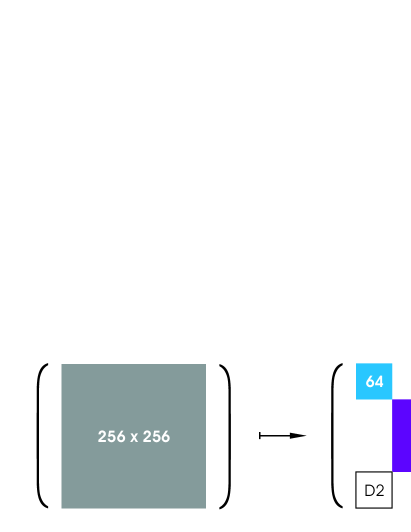
X        $\operatorname{ad}_{H}\hskip 51.21495pt\mapsto\hskip 56.9055pt\big{(}\operatorname{ad}_{H}\big{)}_{\Gamma}$       

Abbildung 2: (Colour online) In a physical four-qubit system for encoding two logical qubits, the Hamiltonians (in their superoperator representations of $\operatorname{ad}_{H}$) take the form of $256\times 256$ matrices. In the eigenbasis of $\Gamma$ (Eqn. 18), the drift Hamiltonian $\operatorname{ad}_{H_{D1}}$ of System I block diagonalises into slowly relaxing modes (blue) with relaxation rate constants in the interval $[0\,s^{-1},0.060\,s^{-1}]$, moderately relaxing modes (magenta) with $[4.01\,s^{-1},4.06\,s^{-1}]$, and fast relaxing modes (red) with $[8.02\,s^{-1},8.06\,s^{-1}]$. In System II the Hamiltonian $\operatorname{ad}_{H_{D1+D2}}$ comprises off-diagonal blocks (empty boxes) that make the protected modes exchange with the fast decaying ones. [NB: for pure $T_{2}$-relaxation (Eqn. 17), the relaxation-rate eigenvalues would further degenerate to $0\,s^{-1}$ (‘decoherence-free’), $4\,s^{-1}$ (medium) and $8\,s^{-1}$ (fast) while maintaining the same block structure].

Model System II

Now, by extending the Ising-ZZ coupling between the two qubit pairs to an isotropic Heisenberg-XXX interaction, one gets what we define as System II. Its drift term with the coupling constants being set to $J_{xx}=2$ Hz and $J_{xyz}=1$ Hz reads

$$\begin{split}H_{D1+D2}\;\;:=\;\;&J_{xx}\,\big{(}xx{\rm 1\negthickspace l}{}{\rm 1\negthickspace l}{}+{\rm 1\negthickspace l}{}{\rm 1\negthickspace l}{}xx+yy{\rm 1\negthickspace l}{}{\rm 1\negthickspace l}{}+{\rm 1\negthickspace l}{}{\rm 1\negthickspace l}{}yy\big{)}\\ +&J_{xyz}\;\;\,\big{(}{\rm 1\negthickspace l}{}xx{\rm 1\negthickspace l}{}+{\rm 1\negthickspace l}{}yy{\rm 1\negthickspace l}{}+{\rm 1\negthickspace l}{}zz{\rm 1\negthickspace l}{}\big{)}\end{split}$$ (22)

and it takes the system out of the decoherence-protected subspace due to the off-diagonal blocks in Fig. 2; so the dynamics finds its Lie closure in a much larger algebra isomorphic to $\mathfrak{so}(12)$,

$$\dim{\langle(H_{D1+D2}),H_{C1},H_{C2}\rangle}_{\rm Lie}=66\;,$$ (23)

to which $\mathfrak{su}(4)$ is but a subalgebra.

Note that $e^{-i\pi H_{C\nu}}(H_{D1+D2})e^{i\pi H_{C\nu}}=H_{D1-D2}$ for either $\nu=1,2$. So invoking Trotter’s formula

$$\lim\limits_{n\to\infty}\big{(}e^{-i(H_{D1+D2})/(2n)}e^{-i(H_{D1-D2})/(2n)}\big{)}^{n}=e^{-iH_{D1}}$$ (24)

it is easy to see that the dynamics of System II may reduce to the subspace of System I in the limit of infinitely many switchings of controls $H_{C1}$ or $H_{C2}$ and free evolution under $H_{D1+D2}$. It is in this decoupling limit that System II encodes a fully controllable logical two-qubit system over the then dynamically protectable basis states of $\mathcal{B}\otimes\mathcal{B}$.

In the following paragraph we may thus compare the numerical results of decoherence-protection by optimal control with alternative pulse sequences derived by paper and pen exploiting the Trotter limit. As an example we choose the CNOT gate in a logical two-qubit system encoded in the protected four-qubit physical basis $\mathcal{B}\otimes\mathcal{B}$.

X     (a)                                                     (b)                                                                                                                               
        

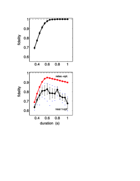
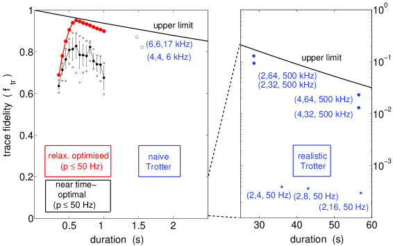
Abbildung 3: (Colour online) Fidelity of a CNOT gate encoded in an open system of four physical qubits in different scenarios of System II (see text). For reference, the top panel of (a) shows the top curve $g_{0}(T)$ consisting of maximum obtainable fidelities against fixed final time $T$ in the absence of relaxation; mean and rmsd are shown for families of 15 independent control sequences generated for each $T$. The lower panel of (a) shows their performance vastly scattering in the presence of relaxation ($\bullet$) with the intervals giving mean $\pm$ rmsd for all the $15$ control sequences tested (dots for best and worst values), while numerical optimal control under explicit relaxation ($\bullet$) is far superior. In (b) these results are compared with ($\mathbf{\circ}$) by naive Trotter calculations assuming to every interaction the inverse is directly obtainable; ($\bullet$) depicts a realistic Trotter approach, where the inverse has to be explicitly generated. The numbers in brackets $(n_{1},n_{2},p)$ give the expansion coefficients $n_{1},n_{2}$ of Fig. 5 and the max. control power $p$ (counted as number of $2\pi$-rotations per second). Note that numerical optimal control requires some four orders of magnitude less power than the bang-bang type decoupling from fast relaxing modes used in the Trotter expansions. The upper quality limit is imposed by slow $T_{1}$-type relaxation (see text). Without relaxation, all the Trotter sequences would achieve fidelities between $93$ and $99$ %, except ($\star$) the ones limited to control fields of powers $p\leq\,50$ Hz: they would fall below $5$%.

III.2 Results on Performing Target Operations under Simultaneous Decoupling

The model systems are completely parameterised by their respective Master equations, i.e. by putting together the Hamiltonian parts of Eqns. (20) for System I or Eqn. (22) for System II and the relaxative part expressed in Eqn. (18). We will thus compare different scenarios of approximating the logical CNOT target gate ($\operatorname{Ad}_{U_{\rm CNOT}}$) by the respective quantum map $F(T)$ while at the same time, the logical two-qubit subsystem has to be decoupled from the fast decaying modes in order to remain within a weakly relaxing subspace. This is what makes it a demanding simultaneous optimisation task. — The numerical and analytical results are summerised in Fig. 3; they come about as follows.

III.2.1 Comparison of Relaxation-Optimised and Near Time-Optimal Controls

With decoherence-avoiding numerically optimised controls one obtains a fidelity beyond $95\%$, while near time-optimal controls show a broad scattering as soon as relaxation is taken into account: among the family of 15 sequences generated, serendipity may help some of them to reach a quality of $85$ to $90\%$, while others perform as bad as giving $65\%$. With opengrape performing about two standard deviations better than the mean obtained without taking relaxation into account, only $2.5\%$ of near time-optimal control sequences would roughly be expected to reach a fidelity beyond $95\%$ just by chance. Fig. 4 then elucidates how the new decoherence avoiding controls keep the system almost perfectly within the slowly-relaxing subspace, whereas conventional near time-optimal controls partly sweep through the fast-relaxing subspace thus leading to inferior quality.

(a)                                                   (b)                                                      

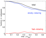
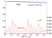
Abbildung 4: (Colour online) (a) Time evolution of all the protected basis states under a typical time-optimised control of Fig.3. Projections into the slowly-relaxing and fast-relaxing parts of the Liouville space are shown. (b) Same for the new decoherence-avoiding controls. System II (see text) then stays almost entirely within the $T_{2}$-protected subspace.

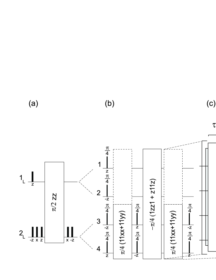
Abbildung 5: Impractical academic alternative to numerical control: the algebraic derivation of controls for a CNOT in the slowly-relaxing subspace proceeds from (a) the logical two-qubit system via (b) the encoded schematic physical four-qubit system to the physical realisations in the settings of (c) System I and (d) System II as defined in the text. Note that by the definition of the encoding Bell states (Eqn. 14) all angles halve upon going from (a) to (b). Effective Hamiltonians $\tau H$ are represented by large frames; $n_{1},n_{2}$ indicate repetitions for the respective Trotter expansions. Black bars are local $\tfrac{\pi}{2}$-pulses with phases given as subscript unless other rotation angles given on top; empty bars denote local $z$-rotations by flip angle $\pi$. These pulses can be seen as bang-bang type controls; due to the high repetition rates ($n_{1}=2$ but $n_{2}=64$) the Trotter expansions accumulate field strengths of $p\simeq 500$ kHz, while the pulse shapes from optimal control require $p\leq 50$ Hz. Expanding the interior Hamiltonian in (b) is even more complicated (not shown here)

III.2.2 Comparison to Paper-and-Pen Solutions

Algebraic alternatives to numerical methods of optimal control exploit Trotter’s formula for remaining within the slowly-relaxing subspace when realising the target, see, e.g. Storcz et al. (2005). Though straightforward, they soon become unhandy as shown in Fig. 5. Assuming for the moment that to any evolution under a drift $H_{d}$ the inverse evolution under $-H_{d}$ is directly available, the corresponding “naive” expansions take almost 3 times the length of the numerical results, yet requiring much stronger control fields ($1-17$ kHz instead of $50$ Hz) as shown in Fig. 3. In practice, however, the inverse is often not immediately reachable, but will require waiting for periodicity. For instance, in the Trotter decomposition of Fig. 5 (c), the Ising term $H_{ZZ}:={\rm 1\negthickspace l}{}zz{\rm 1\negthickspace l}{}$ as part of the drift Hamiltonian $H_{D1+D2}$ is also needed with negative sign so that all terms governed by $J_{xyz}$ in Eqn. 22 cancel and only the Heisenberg-XX terms governed by $J_{XX}$ survive. But $H_{ZZ}$ cannot be sign-reversed directly by the $z$-controls in the sense ${\rm 1\negthickspace l}{}zz{\rm 1\negthickspace l}{}\mapsto-{\rm 1\negthickspace l}{}zz{\rm 1\negthickspace l}{}$ since it clearly commutes with the $z$-controls. Thus one will have to choose evolution times ($\tau_{2}$ in Fig. 5) long enough to exploit (quasi) periodicity. However, $H_{D1+D2}$ shows eigenvalues lacking periodicity within practical ranges altogether. Moreover, the non-zero eigenvalues of $H_{D1+D2}$ do not even occur in pairs of opposite sign, hence there is no unitary transform $U:H\mapsto-H=UAU^{\dagger}$ to reverse them, and a forteriori there is no local control that could do so either Schulte-Herbrüggen and Spörl (2006).

Yet, when shifting the coupling to $J_{xx}=2.23$ Hz to introduce a favourable quasi-periodicity, one obtains almost perfect projection ($f_{\operatorname{tr}}\geq 1-10^{-10}$) onto the inverse drift evolution of System II, to wit $U^{-1}:=e^{+i\tfrac{\pi}{4}H_{D_{1}+D_{2}}}$ after $3.98$ sec and onto $-U^{-1}$ after $1.99$ sec. Thus the identity $\operatorname{Ad}_{(-U^{-1})}=\operatorname{Ad}_{(U^{-1})}$ may be exploited to cut the duration for implementing $\operatorname{Ad}_{U^{-1}}$ to $1.99$ sec. Yet, even with these facilitations, the total length required for a realistic Trotter decomposition (with an overall trace fidelity of $f_{\rm tr}\geq 94.1$ % in the absence of decoherence) amounts to some $28.5$ sec as shown in Fig. 3. Moreover, as soon as one includes very mild $T_{1}$-type processes, the relaxation rate constants in the decoherence-protected subspace are no longer strictly zero (as for pure $T_{2}$-type relaxation), but cover the interval $[0\,{\rm s}^{-1},0.060\,{\rm s}^{-1}]$. Under these realistic conditions, a Trotter expansion gives no more than $15$% fidelity, while the new numerical methods allow for realisations beyond $95$% fidelity in the same setting (even with the original parameter $J_{xx}=2.0$ Hz).

IV Discussion

In order to extract strategies of how to fight relaxation by means of optimal control, we classify open quantum systems (i) by their dynamics being Markovian or non-Markovian and (ii) by the (Liouville) state space directly representing logical qubits either directly without encoding or indirectly with one logical qubit being encoded by several physical ones. So the subsequent discussion will lead to assigning different potential gains to different scenarios as summerised in Table 1.

Before going into them in more detail, recall (from the section on numerical setting) that the top curve $g_{0}(T)$ shall denote the maximum fidelity against final times $T$ as obtained for the analogous closed quantum system (i.e. setting $\Gamma=0$) by way of numerical optimal control. Moreover, define $T_{*}$ as the smallest time such that $g_{0}(T_{*})=1-\varepsilon$, where $\varepsilon$ denotes some error-correction threshold.

First (I), consider the simple case of a Markovian quantum system with no encoding between logical and physical qubits, and assume $g_{0}(T)$ has already been determined. If as a trivial instance (I.a) one had a uniform decay rate constant $\gamma$ so $\Gamma=\gamma{\rm 1\negthickspace l}{}$, then the fidelity in the presence of relaxation would simply boil down to $f(T)=g_{0}(T)\cdot e^{-T\cdot\gamma}$. Define $T^{\prime}_{*}:=\operatorname{argmax}\{f(T)\}$ and pick the set of controls leading to $g_{0}(T^{\prime}_{*})$ calculated in the absence of relaxation for tracking $g_{0}(T)$. In the simplest setting, they would already be ‘optimal’ without ever having resorted to optimising an explicitly open system. More roughly, the time-optimal controls at $T=T_{*}$ already provide a good approximation to fighting relaxation if $T_{*}-T^{\prime}_{*}\geq 0$ is small, i.e. if $\gamma>0$ is small.

Next consider a Markovian system without coding, where $\Gamma\neq\gamma{\rm 1\negthickspace l}{}$ is not fully degenerate (I.b). Let $\{\gamma_{j}\}$ denote the set of (the real parts of the) eigenvalues of $\Gamma$. Then, by convexity of $\{e^{-\gamma t}\;|\;t,\gamma>0\}$, the following rough yet useful limits to the fidelity $f(T)$ obtainable in the open system apply

$$g_{0}(T)\cdot\exp\{-\frac{T}{N^{2}}\sum_{j=1}^{N^{2}}\gamma_{j}\}\lesssim f(T)\lesssim g_{0}(T)\cdot\frac{1}{N^{2}}\sum_{j=1}^{N^{2}}e^{-\gamma_{j}T}\;.$$ (25)

Hence the optimisation task in the open system amounts to approximating the target unitary gate ($\operatorname{Ad}_{U_{\rm target}}$) by the quantum map $F(T)$ resulting from evolution under the controls subject to the condition that modes of different decay rate constants $\gamma_{j}\neq\gamma_{k}$ are interchanged to the least possible amount during the entire duration $0\leq t\leq T$ of the controls. An application of this strategy known in NMR spectroscopy as TROSY Pervushin et al. (1997) makes use of differential line broadening Griffey and Redfield (1987) and partial cancellation of relaxative contributions. Clearly, unless the eigenvalues $\gamma_{j}$ do not significantly disperse, the advantage by optimal control under explicit relaxation will be modest, since the potential gain in this scenario relates to the variance $\sigma^{2}(\{\gamma_{j}\})$.

Tabelle 1: Gain Potential for Relaxation-Optimised Controls versus Time-Optimised Controls

Category		Markovian		non-Markovian
encoding:
protected subspace		big		(difficult)
no encoding:
full Liouville space		small–medium		medium–big Rebentrost et al. (2009)

The situation becomes significantly more rewarding when moving to the category (II) of optimisations restricted to a weakly relaxing (physical) subspace used to encode logical qubits. A focus of this work has been on showing that for Markovian systems encoding logical qubits, the knowledge of the relaxation parameters translates into significant advantages of relaxation-optimised controls over time-optimised ones. This is due to a dual effect: opengrape readily decouples the encoding subsystem from fast relaxing modes while simultaneously generating a quantum map of (close to) best match to the target unitary. Clearly, the more the decay of the subspace differs from its embedding, the larger the advantage of relaxation-optimised control becomes. Moreover, as soon as the relaxation-rate constants of the protected subsystem also disperse among themselves, modes of different decay should again only be interchanged to the least amount necessary—thus elucidating the very intricate interplay of simultaneous optimisation tasks that makes them prone for numerical strategies.

In contrast, in the case of entirely unknown relaxation characteristics, where, e.g., model building and system identification of the relaxative part is precluded or too costly, we have demonstrated that guesses of time-optimal control sequences as obtained from the analogous closed system may—just by chance—cope with relaxation. This comes at the cost of making sure a sufficiently large family of time-optimal controls is ultimately tested in the actual experiment for selecting among many such candidates by trial and error—clearly no more than the second best choice after optimal control under explicitly known relaxation.

In the non-Markovian case, however, it becomes in general very difficult to find a common weakly relaxing subspace for encoding (II.b): there is no Master equation of GKS-Lindblad form, the $\Gamma(t)$ of which could serve as a guideline to finding protected subspaces. Rather, one would have to analyse the corresponding non-Markovian Kraus maps for weakly contracted subspaces allowing for encodings. — However, in non-Markovian scenarios, the pros of relaxation-optimised control already become significant without encoding as has been demonstrated in Rebentrost et al. (2009).

Simultaneous Transfer in Spectroscopy

Finally, note that the presented algorithm also solves (as a by-product) the problem of simultaneous state-to-state transfer that may be of interest in coherent spectroscopy Glaser et al. (1998). While Eqns. 9 and 11 refer to the full-rank linear image $F$, one may readily project onto the states of concern by the appropriate projector $\Pi$ to obtain the respective dynamics and quality factor of the subsystem

$$\Pi\;\dot{F} = -\Pi\;(i\operatorname{ad}_{H}\,+\,\Gamma)\;\circ\;F$$ (26)

$$f^{(\Pi)}_{\rm tr} = \tfrac{1}{\operatorname{rk}\Pi}\;\operatorname{Re}\,\operatorname{tr}\{\Pi^{t}\;F_{\rm target}^{\dagger}\Pi\;F(T)^{\phantom{\dagger}}\}$$ (27)

reproducing Eqn. 8 in the limit of $\Pi$ being a rank-1 projector. While such rank-1 problems under relaxation were treated in Khaneja et al. (2003), the algorithmic setting of opengrape put forward here allows for projectors of arbitrary rank, e.g., $1\leq\operatorname{rk}\Pi\leq N$ for $n$ spin-$\tfrac{1}{2}$ qubits with $N:=2^{n}$. Clearly, the rank equals the number of orthogonal state-to-state optimisation problems to be solved simultaneously.

V Conclusions and Outlook

We have provided numerical optimal-control tools to systematically find near optimal approximations to unitary target modules in open quantum systems. The pros of relaxation-optimised controls over time-optimised ones depend on the specific experimental scenario. We have extensively discussed strategies for fighting relaxation in Markovian and non-Markovian settings with and without encoding logical qubits in protected subspaces. Numerical results have been complemented by algebraic analysis of controllability in protected subspaces under simultaneous decoupling from fast relaxing modes.

To complement the account on non-Markovian systems in Rebentrost et al. (2009), the progress is quantitatively exemplified in a typical Markovian model system of four physical qubits encoding two logical ones: when the Master equation is known, the new method is systematic and significantly superior to near time-optimal realisations, which in turn are but a guess when the relaxation process cannot be quantitatively characterised. In this case, testing a set of $10-20$ such near time-optimal control sequences empirically is required for getting acceptable results with more confidence, yet on the basis of trial and error. As follows by controllability analysis, Trotter-type expansions allow for realisations within slowly-relaxing subspaces in the limit of infinitely many switchings. However, in realistic settings for obtaining inverse interactions, they become so lengthy that they only work in the idealised limit of both $T_{2}$ and $T_{1}$-decoherence-free subspaces, but fail as soon as very mild $T_{1}$-relaxation processes occur.

Optimal control tools like opengrape are therefore the method of choice in systems with known relaxation parameters. They accomplish decoupling from fast relaxing modes with several orders of magnitude less decoupling power than by typical bang-bang controls. Being applicable to spin and pseudo-spin systems, they are anticipated to find broad use for fighting relaxation in practical quantum control. In a wide range of settings the benefit is most prominent when encoding the logical system in a protected subspace of a larger physical system. However, the situation changes upon shifting to a timevarying $\Gamma(t)$ Grace et al. (2007), or to more advanced non-Markovian models with $\Gamma\big{(}u(t)\big{)}$ depending on time via the control amplitudes $u(t)$ on timescales comparable to the quantum dynamic process. Then the pros of optimal control extend to the entire Liouville space, as shown in Rebentrost et al. (2009).

In order to fully exploit the power of optimal control of open systems the challenge is shifted to (i) thoroughly understanding the relaxation mechanisms pertinent to a concrete quantum hardware architecture and (ii) being able to determine its relaxation parameters to sufficient accuracy.