Path integrals and boundary conditions

The path integral approach to quantum mechanics provides a method of quantization of dynamical systems directly from the Lagrange formalism. In field theory the method presents some advantages over Hamiltonian quantization. The Lagrange formalism preserves relativistic covariance which makes the Feynman method very convenient to achieve the renormalization of field theories both in perturbative and non-perturbative approaches. However, when the systems are confined in bounded domains we shall show that the path integral approach does not describe the most general type of boundary conditions. Highly non-local boundary conditions cannot be described by Feynman’s approach. We analyse in this note the origin of this problem in quantum mechanics and its implications for field theory.

1 Introduction

The original Heisenberg formulation of quantum mechanics has been complemented with two equivalent pictures: Schrödinger wave mechanics and Feynman’s path integral. Dirac proved that the Heisenberg and Schrödinger pictures both based on the Hamiltonian approach were equivalent. Feynman’s path integral method although based on the Lagrangian formalism is also equivalent to the other two formulations for most quantum mechanical systems Feynman ; Feynman-Higgs . In field theory Feynman’s formulation proved to be very useful. In perturbation theory, the explicit covariant character of its natural functional integral generalization makes possible a simpler approach to the renormalization of ultraviolet divergences. In the Euclidean version FeyKac the functional integral formulation is a crucial ingredient for non-perturbative approaches to field theory and critical phenomena wilson . The equivalence of the functional integral formulation with the Hamiltonian pictures also holds for constrained systems like gauge theories and string theories. The ordering ambiguity problem of Hamiltonians in constrained systems has also an analytic counterpart in the functional method. Indeed, Ito and Stratonovich discretizations of path integrals provide different prescriptions for quantum systems. However, there is an exception to this rule. For systems constrained to bounded domains the Feynman approach does not describe the most general type of boundary conditions compatible with Hamiltonian approaches sant . The analysis of this problem is the main goal of this note.

On the other hand the physics of boundary conditions is becoming very relevant in quantum gravity, string theory and brane theory. A large variety of boundary conditions are required to describe new physical effects. The limitations of the scope of functional integral methods might require new methods to describe these phenomena. Effects like anomalies anm ; aae ; esteve topology change rbal quantum holography bek ; qg ; hol , quantum gravity and AdS/CFT correspondence mal show the relevance of boundaries in the description of fundamental physical phenomena. Moreover, the recent observation of a suppression of quadropole and octopole components of the cosmic background radiation might be connected with the boundary conditions or the space topology of the Universe dod . To some extent the role of boundary phenomena has been promoted from academic and phenomelogical simplifications of complex physical systems to a higher status connected with very basic fundamental principles. Thus, the issue of whether the path integral approach is able to describe all boundary effects is very important. Otherwise, the analysis of non-perturbative effects under generic boundary conditions must rely in new non-perturbative Hamiltonian methods.

2 Quantum boundary conditions

Probability preservation is the fundamental quantum dynamical principle which imposes the more severe constrains on the boundary conditions of systems evolving in bounded domains. The analytical condition, which is encoded by self–adjointness of the Hamiltonian operator, contains all the quantum subtleties associated to the unitarity principle and the dynamical behaviour at the boundary.

The existence of a boundary generically enhances the genuine quantum aspects of the system. Famous examples of this enhancement are the Young two slits experiments and the Aharanov-Bohm effect, which pointed out the relevance of boundary conditions in the quantum theory. Another examples of quantum physical phenomena which are intimately related to boundary conditions are the Casimir effect cas ; vac the role of edge states sr and the quantization of conductivity qcd ; 9bis in the quantum Hall effect.

Let us consider a point-like particle moving on a bounded domain $\Omega$ of $\hbox{\af R}^{n}$ with regular and oriented boundary $\partial\Omega$. The Schrödinger picture prescribes that the Hamiltonian is given from the scalar Laplacian $\Delta$. This operator is symmetric on the domain of smooth functions with compact support on $\Omega$. However, in this domain the operator is not self–adjoint as it is required by the unitarity quantum principle of time evolution. Now, the Hamiltonian operator can be extended to a larger domain of functions where it becomes self–adjoint. The extension, however, is not unique. The classification of self–adjoint extensions of the Hamiltonian can be characterized in terms of unitary operators between defect subspaces in the classical theory due to von Neumann ds ; gp . However, there is a more useful characterization of these selfadjoint extensions in terms of constraint conditions on the boundary values of the wave functions aim . In this framework the set of self–adjoint extensions of the Hamiltonian is in one-to-one correspondence with the group of unitary operators of the space $L^{2}(\partial\Omega)$ of square integrable functions of the boundary $\partial\Omega$.

Thus, any unitary operator $U$ on the space of boundary functions which are square integrable with respect to the standard Riemaniann measure $d\mu_{{}_{\partial\Omega}}$ induced from the Euclidean metric of $\hbox{\af R}^{n}$ defines a selfadjoint of the quantum Hamiltonian $\Delta^{U}$. Conversely, any selfadjoint extension of $\Delta$ is associated to one unitary operator of this type aim .

The domain of the selfadjoint Hamiltonian governed by $U$ is defined by the wave functions which satisfy the boundary condition

$$\varphi-i\dot{\varphi}=U(\varphi+i\dot{\varphi})$$ (1)

where $\varphi=\psi|_{\partial\Omega}$ is the boundary value of the wave function $\psi$ and $\dot{\varphi}$ its oriented normal derivative at the boundary $\partial\Omega$. The condition (1) implies the vanishing of the boundary term remaining after integration by parts and use of Stokes theorem which is of the form aim

$$\langle\psi_{1},\Delta\psi_{2}\rangle=\langle\Delta\psi_{1},\psi_{2}\rangle+i\int_{\partial\Omega}\,\left[(\dot{\varphi}_{1},\varphi_{2})-(\varphi_{1},\dot{\varphi}_{2})\right]d\mu_{{}_{\partial\Omega}}.$$

Through the above characterization, the set of self–adjoint extensions of the Hamiltonian inherits the group structure of the group of unitary operators. For the half–line the group is $U(1)$ and for a closed interval $U(2)$. For spaces of dimension higher than one the group of boundary conditions is an infinite dimensional group. There are two particular subsets of boundary conditions which can be very explicitly expressed in terms of boundary values. If the spectrum of $U$ does not contain $1$ and $-1$, the boundary conditions (1) reduce to

$${\varphi=A_{-}\dot{\varphi};\qquad{\rm or}\qquad\dot{\varphi}=A_{+}\varphi}$$

where $A_{\pm}$ are the hermitian operators defined by the Cayley transform

$$A_{-}=i{\hbox{\af I }+U\over\hbox{\af I }-U}\qquad A_{+}=-i{\hbox{\af I }-U\over\hbox{\af I }+U}$$

Notice that the set of boundary conditions where the Cayley transform becomes singular include two well known types of boundary conditions: Dirichlet ($U=-\hbox{\af I }$) and Neumann ($U=\hbox{\af I }$) boundary conditions. But the group of boundary conditions is much larger. In particular, for two dimensional and higher dimensional systems bounded to compact domains the space of selfadjoint extensions is a infinite-dimensional manifold. The quantum role of boundary conditions is very important for the behaviour of low energy levels. High energy levels are quite independent of boundary effects. Indeed, boundary effects play no role in the ultraviolet regime, whereas they are crucial for the infrared. In particular, the existence of edge states is only possible under certain boundary conditions. A very important result concerning edge states is that if the unitary operator $U$ characterizing the selfadjoint extension has one eigenvalue $-1$ with smooth eigenfunction, the selfadjoint extensions associated to $U_{t}=U{\rm e}^{it}$ have for small values of $t$ one negative energy level which corresponds to an edge state. The energy of this edge state becomes infinite when $t\to 0$ aim . In this case all the negative bounding energy is provided by the boundary.

3 Boundary conditions in path integrals

The action principle governs the classical and quantum dynamics of unconstrained systems. The classical dynamics is given by stationary trajectories from the variational action principle and the quantum dynamics is automatically implemented in the path integral formalism by the weight that the classical action provides for classical trajectories. However, for particles evolving in a bounded domain the variational problem is not uniquely defined. It is necessary to specify the evolution of the particles after reaching the boundary. The constraints that appear on the trajectories contributing to the path integral only depend on the very nature of the physical boundary.

In fact, the nature of the boundary imposes more severe constraints on the classical dynamics than to the quantum evolution. This is due to the point-like nature of the particle which requires that after reaching the boundary the individual particle has to emerge either back at the same boundary point or at a different point of the same boundary. The only allowed freedom is where it emerges back and the momentum it emerges with. The emergence of the particle at a different point covers the possibility that the domain be folded and glued at the apparent boundary giving rise to non-trivial topologies. In summary, the classical boundary conditions are given by two maps: an isometry of the boundary

$$\alpha:\partial\Omega\to\partial\Omega$$

and a positive density function

$$\rho:\partial\Omega\to{\rm\hbox{\af R}^{+}}$$

which specify the change of position and normal component of momentum of the trajectory of the particle upon reaching the boundary. The isometry $\alpha$ encodes the possible geometry and topology generated by the folding of the boundary and the function $\rho$ is associated to the reflectivity (transparency or stickiness) properties of the boundary. Once these two functions are specified the classical variational problem is restricted to trajectories which satisfy the boundary conditions:

$${\bf{\bf x}}(t_{+})=\alpha({\bf x}(t_{-})),$$ (2)

$${\bf n}({\bf x}(t_{+})))\cdot\dot{\bf x}(t_{+})=-\rho({\bf x}(t_{-}))\,{\bf n}({\bf x}(t_{-}))\cdot\dot{\bf x}(t_{-})$$ (3)

and

$$\alpha_{\ast}(\dot{\bf x}(t_{-})-[{\bf n}({\bf x}(t_{-}))\cdot\dot{\bf x}(t_{-})]\,{\bf n}({\bf x}(t_{-}))$$

$$\phantom{adadfa}=\dot{\bf x}(t_{+})-[{\bf n}({\bf x}(t_{+}))\cdot\dot{\bf x}(t_{+})]\,{\bf n}({\bf x}(t_{+})$$ (4)

for any $t$ such that ${\bf x}(t)\in\partial\Omega$, where ${\bf n}$ denotes the exterior normal derivative at the boundary $\partial\Omega$ and

$${\bf x}(t_{\pm})=\lim_{s\to 0}{\bf x}(t\pm s).$$

This definition of classical boundary conditions is motivated by the standard physical heuristic interpretation of boundary conditions. Linear momentum is not conserved because it is partially or totally absorbed by the boundary. The major constraints on the choice of boundary conditions arise first from the very notion of point-like particle which requires that any trajectory which reaches the boundary has to emerge as a single trajectory from the same boundary. The second requirement concerning the permitted changes of linear momentum at the boundary is constrained by its compatibilitywith the action principle. This establishes that classical trajectories are determined by the stationary points of the classical action

$$S({\bf x})=\int dt\,g_{ij}{\,\dot{x}^{i}(t)}{\dot{x}^{j}(t)}.$$

The variational principle yields the celebrated Euler-Lagrange motion equations $\ddot{\bf x}(t)=0$ provided that the boundary term

$$\sum_{m=1}^{N}\biggl{[}\delta{\bf x}(t_{m}^{+})\cdot\dot{\bf x}(t_{m}^{+})-\delta{\bf x}(t_{m}^{-})\cdot\dot{\bf x}(t_{m}^{-})\biggr{]}$$ (5)

vanishes, where the sum is over all points $t_{m}$ where the trajectories reach the boundary. The simpler way of fulfilling this requirement is by imposing the vanishing of each individual term on the sum. These conditions reduce to the boundary conditions (3)(3) provided that the only permitted variations are tangent to the boundary. In this case the normal component of $\delta{\bf x}(t_{m})$ vanishes, i.e. the points of trajectories which reach the boundary are only allowed to move along the boundary. This conditions is reminiscent of Dirichlet condition for D-branes in string theory. There is no analogue of the Neumann boundary conditions of strings for point-like particles.

Simple but interesting types of boundary conditions already arise in the Sturm-Liouville problem, $\Omega=[0,1]$. In such a case the boundary of the configuration space is a discrete two-points set, $\partial\Omega=\{0,1\}$. Examples of classical boundary conditions in such a case are

i)   Neumann (total absorption): $\alpha=I$, $\rho(0)=\rho(1)=\infty$.

ii)  Dirichlet (total reflection): $\alpha=I$, $\rho(0)=\rho(1)=1$.

iii) Periodic: $\alpha(0)=1$, $\alpha(1)=0$, $\rho(0)=\rho(1)=1$.

iv) Quasi-periodic: $\alpha(0)=1$, $\alpha(1)=0$, $\rho(0)=\rho(1)=\epsilon$.

The quantum implementation of those boundary condition is straightforward via the path integral method. The only paths to be considered in the Feynman’s path integration are those that satisfy the classical boundary conditions (2)–(3). In the one–dimensional case of Sturm-Liouville problem the space of quantum boundary conditions is a four–dimensional Lie group $U(2)$, whereas the space of classical boundary conditions is the union of two disconnected two–dimensional manifolds,

$${\cal M}_{1} = \{\psi\in L^{2}([0,1]),\dot{\varphi}(0)=({1-\rho_{1}})\varphi(1),\dot{\varphi}(1)=({1-\rho_{0}})\varphi(0)\}$$ (6)

$${\cal M}_{0} = \{\psi\in L^{2}([0,1]),\dot{\varphi}(0)=({1-\rho_{0}})\varphi(0),\dot{\varphi}(1)=({1-\rho_{1}})\varphi(1)\}$$ (7)

Thus, the Feynman path integral approach does not cover the whole set of boundary conditions.

Some quantum boundary conditions which are not of type (6)(7) can be related to periodic boundary conditions (iii) with a singular potential supported at the boundary groscheb . Indeed, the boundary condition associated to the unitary operator

$$U=\frac{1}{2-ia}\pmatrix{{ia}&{2}\cr{2}&{ia}}$$ (8)

can be thought as a delta function potential in a circle, i.e. usual periodic boundary conditions

$$U=\pmatrix{0&1\cr{1}&0}$$

for the Hamiltonian

$$H=-\frac{d^{2}}{dx^{2}}+a\delta(x).$$

In other cases, the boundary conditions can be described by periodic boundary conditions and non-trivial magnetic fluxes, e.g. in the anti-diagonal case

$$U=\pmatrix{0&e^{-i\epsilon}\cr e^{i\epsilon}&0}$$

we have (pseudo)periodic boundary conditions

$${{\varphi(1)=e^{i\epsilon}\varphi(0)\qquad\varphi^{\prime}(1)=e^{i\epsilon}\varphi^{\prime}(0)}}$$

with two opposite probability fluxes propagating across the boundary. This condition is in fact a topological boundary condition which corresponds to fold the interval into a circle $S^{1}$, with a magnetic flux $\epsilon$ crossing through the loop, i.e. the Hamiltonian

$$H=-\left(\frac{d}{dx}-i\epsilon\right)^{2}$$

with standard periodic boundary conditions. The images method also permits to use unconstrained path integral methods to describe systems with non-trivial boundary conditions groschea . However, in this case the use of the path integral is not as simple as in the Feynman original formulation.

But even with these tricks path integral methods do not describe all possible types of boundary conditions even in the simple case of Sturm-Liouville problem. One of reasons behind the failure of path integral picture is the single valued nature of trajectories. Many conditions, e.g. the boundary condition (8) describe a scattering by a singular potential sitting on the circle groscheb . There are two different types of quantum interactions with the boundary: reflection and diffraction. A classical description of the phenomena without including a potential term will require the splitting of the ongoing classical trajectory into two outgoing paths: one pointing forward and another one backwards. This picture destroys the pure point-like particle approach and leads to multivalued trajectories which dramatically changes the simple Feynman’s description of path integrals. Furthermore, there are boundary conditions where one single trajectory upon reaching the boundary has to be split into an infinite set of outgoing trajectories. This behaviour can be explicitly pointed out by noticing that the quantum evolution of a narrow wave packet evolves backward after being scattered by the boundary as a quite widespread wave packet emerging from all points of the boundary.

In higher dimensions the mismatch between the spaces of quantum and classical boundary conditions is even larger sant . It is obvious that there are many quantum boundary conditions that cannot be described by local boundary conditions even with the incorporation of singular potentials which in this case might require renormalization dl ; 0bis One particularly interesting example is provided by a particle moving on an annulus with two circular boundaries (see Figure 1)

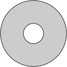
Figure 1: The Corbino disk

with boundary conditions

$$\varphi_{\pm}=\pm\Delta_{\partial\Omega}\,\dot{\varphi}_{\pm}.$$ (9)

In this case there might appear negative energy levels associated to edge states aim . Annular quantum devices (Corbino disks) are used in some quantum Hall effect experiments and the edge states generate chiral currents along the two edges of the disk.

The boundary condition (9) has no path integral description. In summary, the Feynman approach does not describe the whole set of boundary conditions. This fact is a consequence of the enhancement of genuine quantum effects by the presence of the boundary. The boundary itself can be considered from this point of view a genuine quantum device.

4 Conclusions

Highly non-local quantum boundary conditions cannot be described by path integrals. This means that Feynman’s approach to quantum mechanics is not completely equivalent to the Heisenberg and Schrödinger approaches which is a real drawback for the path integral formalism. One may argue that strictly speaking non-locality might never appears in Nature. Boundary conditions for macroscopic boundaries have always a microscopic origin. But even if the fundamental laws of microscopic physics are perfectly local, effective non-local macroscopic conditions can be generated in the presence of matter. The mechanism responsible of the phenomena is similar to what occurs with relativistic invariance. The microscopic laws of the standard model are relativistic invariant. However the presence of matter breaks this invariance and macroscopic objects like cavities and boundaries do exist. Thus, even if the ultimate laws of physics are local, non-local boundary conditions can be achieved by the presence of highly correlated matter boundaries. In such a case the quantum system cannot be described by the path integral formalism.

5 Acknowledgments

This article is dedicated to Alberto Galindo with the occasion of his retirement. His deep knowledge of the most intricate aspects of modern physics and mathematics and his uncompromising comments and opinions played a a crucial role in the development of spanish modern theoretical physics. The Galindo-Pascual book on quantum mechanics gp was one of the very few fundamental books where the problem of boundary conditions was approached from a rigorous viewpoint.

References

- (1) R. P. Feynman, Rev. Mod. Phys. 20 (1948) 367
- (2) R. P. Feynman, and A. R. Hibbs, Quantum mechanics and path integrals, McGraw-Hill, New York, (1965)
- (3) M. Kac, in Proc. 2nd Berkeley Symposium Math. Statist. Probability, Univ. Cal. Press (1950) 189
- (4) K. Wilson, Phys. Rev. D10 (1974)2445
- (5) M. Asorey, in Stochastic processes applied to physics, Ed. L. Pesquera and M.A. Rodriguez, World Sci., Singapore (1985)
- (6) N.S. Manton, Ann. Phys. (N.Y.) 159 (1985) 220
- (7) M. Aguado, M. Asorey and J.G. Esteve, Commun. Math. Phys. 218 (2001) 233
- (8) J.G. Esteve, Phys. Rev. D 34 (1986) 674; Phys. Rev. D66(2002) 125013
- (9) A.P. Balachandran, G. Bimonte, G. Marmo and A. Simoni, Nucl. Phys. B 446 (1995) 299
- (10) J. Bekenstein, Lett. Nuovo Cim. 4 (1972) 737, Phys. Rev. D7 (1973) 2333
- (11) G. t’ Hooft, in Salamfestschrift: A collection of talks, Eds. A. Ali,J. Ellis and S. Randjbar-Daemi World Sci. (1993); Phys. Scripta T36 (1991) 247; Class. Quant.Grav. 16 (1999) 3263
- (12) L. Susskind, J. Math. Phys. 36 (1995)6377
- (13) J. Maldacena, Adv. Theor. Phys. 2(1998) 231
- (14) J.-P. Luminet, A. Riazuelo, R. Lehoucq and J.P. Uzan, Nature 425 (2003) 593
- (15) H.B.G. Casimir, Proc. K. Ned. Akad. Wet. 51(1948) 793
- (16) P. Milonni, The Quantum Vacuum: An Introduction to Quantum Electrodynamics , Academic Press, San Diego (1994)
- (17) V. John, G. Jungman and S. Vaidya, Nucl. Phys. B 455 (1995) 505
- (18) D.J. Thouless, M. Kohmoto, M. P. Nightingale and M. den Nijs, Phys. Rev. Lett. 49 (1982) 405
- (19) J. Avron and R. Seiler, Phys. Rev. Lett. 54 (1985)259
- (20) N. Dunford, J.T. Schwartz, Linear Operators, Part II: Spectral theory, self–adjoint operators in Hilbert space, Wiley, New York (1963)
- (21) A. Galindo and P. Pascual, Quantum mechanics, Springer-Verlag, Berlin, 1990-1991
- (22) M. Asorey, A. Ibort and G. Marmo, Int. J. Mod. Phys. A 12(2004)
- (23) C. Grosche, Phys. Rev. Lett. 71 (1993) 1
- (24) C. Grosche, Annalen Phys.2 (1993) 557
- (25) R. Jackiw, in M.A.B. Bég Memorial Volume, eds. A. Ali and P. Hoodbhoy, World Sci., Singapore (1992)
- (26) C. Manuel and R. Tarrach, Phys. Lett. B 301 (1993) 72