Information transfer rates in spin quantum channels

Abstract

We analyze the communication efficiency of quantum information transfer along unmodulated spin chains by computing the communication rates of various protocols. The effects of temporal correlations are discussed, showing that they can be exploited to boost the transmission efficiency.

I Introduction

Spin networks are an ideal theoretical playground to devise, test and analyze quantum information processing NIELSEN . Examples are the implementation of computational models in spin chains introduced in Refs. computation ; FITZ or the possibility to realize approximate quantum cloners DECHIARA . In the context of quantum communication, several protocols have been proposed which would allow distant parties to exchange and/or share quantum information over chains of permanently coupled spins FITZ ; bose03 ; vittorio05 ; daniel05 ; daniel05B ; daniel05C ; vgdaniel ; OSBORNE ; hase05 ; WOJCIK ; KARBACH ; PATERNOSTRO ; yung ; niko ; DATTA ; DEPASQUALE ; Plenio ; SRINIVASA ; HE ; CAI . This research is in part motivated bose03 by the need of finding alternatives to the standard flying qubits strategies for connecting regions of high control (i.e. quantum computers). These latter approaches, in fact, may pose non trivial interfacing problems with several of the proposed quantum computing architectures (e.g. ion traps, Josephson junctions, etc.). On the other hand, there have been some indications that effective spin networks could be engineered by using arrays of Josephson junctions ROMITO , quantum dots IDAMICO , optical lattices OPTICAL or QED cavities CAVITY .

The ultimate aim of typical communication protocols is to achieve perfect transfer of any quantum state in a given period of time. High degrees of efficiency in these protocols also require the capability of isolating the experimental setup from the external world, preventing it from decoherence, and to reduce all static internal imperfections. Two different strategies are usually adopted: A certain class of schemes achieve efficient communication by tailoring the system Hamiltonian DATTA ; KARBACH ; PATERNOSTRO ; yung ; niko ; Plenio ; SRINIVASA , with a corresponding minimal (if not null) cost in terms of encoding and decoding operations. In the second approach, communication efficiency is obtained through complex encoding and decoding operations but with minimal requirements on the Hamiltonian of the chain OSBORNE ; hase05 ; daniel05 ; daniel05B ; daniel05C ; vgdaniel ; HE ; WOJCIK . Apart from unavoidable experimental noise, which inevitably reduces the fidelity of the state transfer, even the theoretical analysis of these protocols is problematic, because of the dispersive nature of the information propagation OSBORNE ; bose03 . Indeed, on one hand, dispersion does not permit a sharp definition of transmission times, while, on the other hand, it is responsible for the presence of feedback and memory effects MEMORY ; MEMORY1 in the quantum communication.

In this paper we analyze the communication performances of some spin-chain communication protocols. By studying the asymptotic number of qubits transmitted per second, we will show that efficient mechanisms of information transfer can be devised by carefully exploiting the dispersive dynamics of the chain. The paper is organized as follows. In Sec. II we introduce a prototypical spin chain communication model. In Sec. III we show how one can use the internal dynamics of the chain to improve the communication efficiency by focusing on the simplest not-trivial solvable case (i.e. a chain with only two intermediate spins). In Sec. IV instead we analyze the case of arbitrarily long chains: here a lower bound on the attainable communication rates is provided by exploiting the dual-rail protocol of Ref. daniel05 . Finally, in Sec. V we draw our conclusions.

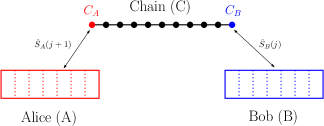
Figure 1: Communication scenario. Alice (A) and Bob (B) control their memory, and have access respectively to the first and the last qubit of the chain (C). The intermediate spins of the chain act as a quantum channel for quantum communication between Alice and Bob. At regular time intervals both Alice and Bob perform a SWAP gate between one of her/his memory qubit and the spin of the chain to whom each of them has access. During the time between two consecutive swaps the chain is let freely evolve, according to the Hamiltonian $\hat{\mathcal{H}}$.

II The model

As in Refs. bose03 ; vittorio05 ; daniel05 ; daniel05B ; daniel05C ; vgdaniel ; OSBORNE ; hase05 ; WOJCIK , the spin communication channel we consider here is an array $C$ of $N$ permanently coupled spin $1/2$ that interact through an Hamiltonian $\hat{\mathcal{H}}$. The total spin component $\hat{S}_{z}$ of the system (e.g. ferromagnetic Heisenberg or $XY$ interaction) is a constant of motion. The chain $C$ constitutes the physical channel along which quantum information is transmitted. As shown in Fig. 1, we assume that the sender (Alice) and the receiver (Bob) of the messages have access to two distinct subsets $C_{A}$ and $C_{B}$ of the spins of the chain (typically the first and the last spin) and to two distinct sets of ancillary qubits (i.e. Alice’s memories $A\equiv\cdots A_{3}\;A_{2}\;A_{1}$ and Bob’s memories $B\equiv B_{1}\;B_{2}\;B_{3}\;\cdots$, respectively). Such subsets and memories are used to “write” and “read” the information into and from the chain, and constitute areas of complete control for the communicating parties (namely Alice has total control on $A+C_{A}$, while Bob has total control on $B+C_{B}$).

In the communication scenario we are considering here the spins of the chain and Bob’s memories $B$ are initially set up in the $\hat{\sigma}_{z}$ “down” state $\left|0\right\rangle\equiv\left|\downarrow\right\rangle$ (analogously we indicate the $\hat{\sigma}_{z}$ “up” vector with $\left|1\right\rangle\equiv\left|\uparrow\right\rangle$). On the other hand Alice’s memories $A$ are in some (possibly entangled) input states $|\Psi\rangle_{A}$ which encode the information she wants to transmit. At time $t=0$ the global state of the composite system $A+C+B$ is thus

$$|\Psi\rangle_{A}\otimes|{\bf 0}\rangle_{C}\otimes|{\bf 0}\rangle_{B}\;,$$ (1)

(which is an eigenstate of the Hamiltonian of the chain $\hat{\cal H}$). Ideally, Alice’s and Bob’s goal is to transform (1) into the state

$$|{\bf 0}\rangle_{A}\otimes|{\bf 0}\rangle_{C}\otimes|\Psi\rangle_{B}\;,$$ (2)

by performing local operations on $A+C_{A}$ and $B+C_{B}$ and by cleverly exploiting the transport properties of the chain free evolution. In this context the efficiency of the communication can be characterized through the transmission rate $r$ of the protocol. This is an asymptotic quantity which describes the maximum number of qubits one can transfer per unit of time with average fidelity converging to $1$ in the limit of large transmission times (see for instance MEMORY ). In the present paper however, we will mostly focus on protocols for which the average time ${T}$ it takes to pass from (1) to (2) is a finite quantity. In this case $r$ is given by

$$r=M/{T}\;,$$ (3)

where $M$ is the number of qubits encoded into the states $|\Psi\rangle_{A}$ of Eq. (1). In what follows ${T}$ will be computed by considering only the spin chain free evolution, thus neglecting the time intervals employed by Alice and Bob to perform their local operations. This is legitimate by the fact that in the model the only dynamical constraint is imposed by $\hat{\cal H}$.

Even in the ideal case when the coupling with the environment and the presence of imperfections is neglected, the evaluation of the transmission rate of Eq. (3) is typically complicated by the dispersive free evolution of the chain OSBORNE ; vgdaniel ; bose03 ; daniel05 ; daniel05B ; daniel05C ; vittorio05 . To better understand this point it is sufficient to focus on the case in which $|\Psi\rangle_{A}$ is a separable vector of the form

$$|\Psi\rangle_{A}=|\cdots\;\psi_{3}\;\psi_{2}\;\psi_{1}\rangle_{A}$$ (4)

where the $j$-th memory element of Alice’s memory is initialized in $|\psi_{j}\rangle_{A_{j}}\equiv\alpha_{j}|0\rangle_{A_{j}}+\beta_{j}|1\rangle_{A_{j}}$. Suppose now that Alice starts the transfer protocol at time $t=0$ by coupling her first memory element $A_{1}$ with the chain spin $C_{A}$ through an instantaneous SWAP gate NIELSEN $\hat{S}_{A}(1)$. This resets the memory element $A_{1}$ to $|0\rangle_{A_{1}}$ while “copying” its initial state into the first chain element, i.e.

$$|{\bf\Psi\,0\,0}\rangle_{ACB} \rightarrow |\cdots\;\psi_{3}\;\psi_{2}\;0\rangle_{A}\otimes\;\big{(}\;\alpha_{1}\;|00\cdots 00\rangle_{C}$$ (5)

$$+\beta_{1}\;|10\cdots 00\rangle_{C}\;\big{)}\otimes|{\bf 0}\rangle_{B}\;.$$

The system then evolves freely for a time interval $\tau$ in order to allow the “perturbation” $\psi_{1}$ introduced locally by Alice in $C_{A}$ to spread along the whole chain. Since the Hamiltonian $\hat{\cal H}$ commutes with $\hat{\cal S}_{z}$, the state (5) becomes bose03 :

$$|\cdots\psi_{3}\psi_{2}0\rangle_{A}\otimes\left(\,\alpha_{1}|{\bf 0}\rangle_{C}+\beta_{1}\sum_{n=1}^{N}\gamma_{1n}(\tau)|{\bf n}\rangle_{C}\,\right)\otimes|{\bf 0}\rangle_{B}\;,$$

where $|{\bf n}\rangle_{C}$ represents the state of the chain having all spins down but the $n$-th, and where

$$\gamma_{1n}(\tau)={{}_{C}\langle{\bf n}|}e^{-i\hat{\cal H}\tau/{\hbar}}|{\bf 1}\rangle_{C}$$ (6)

is the probability amplitude of finding the spin up in the $n$-th chain location. By applying the instantaneous SWAP gate $\hat{S}_{B}(1)$ which couples his first memory $B_{1}$ and the last chain element $C_{B}$, Bob has now a chance to transfer Alice’s information into $B$. If the chain Hamiltonian $\hat{\mathcal{H}}$ is engineered such that there exists a certain time $\tau_{*}$ at which the amplitude $\gamma_{1N}(\tau_{*})$ is unitary DATTA (i.e. $\gamma_{1N}(\tau_{*})=e^{i\varphi_{*}}$), then the excitation sent by Alice has been perfectly traveled to the spin $C_{B}$. Bob can thus safely transfer the exact state $\psi_{1}$ into $B_{1}$ with a simple swap operation, followed by a proper phase shift gate on $B_{1}$ to compensate $e^{i\varphi_{*}}$. This process can be iterated to the remaining memories $A$: at the $j$-th run Alice will move the memory $A_{j}$ into the chain by means of the SWAP $\hat{S}_{A}(j)$ which couples $A_{j}$ with $C_{A}$ while, after a time interval ${\tau_{*}}$, Bob will extract it from $C$ by applying the SWAP $\hat{S}_{B}(j)$ which couples $B_{j}$ with $C_{B}$. Assuming perfect timing, the scheme guarantees the transfer of one qubit every ${\tau_{*}}$ seconds, yielding a rate (3) equal to $1/{\tau_{*}}$.

Unfortunately for a generic Hamiltonian $\hat{\mathcal{H}}$ and time $\tau$ the amplitude $\gamma_{1N}(\tau)$ is not unitary; in this case Bob’s SWAP will not succeed in perfectly extracting Alice’s information $\psi_{1}$ out of the chain. The excitation which codifies $\psi_{1}$, that has been previously put into the chain, is in general spread out over all the sites of the chain. Therefore, at each run only a fraction of Alice’s information is transferred in $B$: the rest remains into the chain and has a chance of interfering with the subsequent operations of the communicating parties. In particular, every time Alice couples her memories with the chain, there is a finite probability that part of the information which was previously injected into $C$, will re-enter into $A$. In this case she will never send it back through the chain, so that Bob will never be able to reconstruct the state with perfect fidelity. The net result is the arising of memory effects MEMORY ; MEMORY1 in the communication which require a proper handling.

III Two-spins chain channel

In this section we focus on the simplest non trivial spin channel model. It is given by a chain $C$ of only $N=2$ spins, the first being controlled by Alice and the second by Bob. We will see that, despite its simplicity, the model retains sufficient structure to permit the analysis of memory effects. In particular it will allow us to compare the transmission rates of protocols which exploit memory effects with protocols which do not.

III.1 Plain scheme

We begin by considering a communication scheme where, every $\tau$ seconds, Alice and Bob simultaneously NOTA perform sequences of SWAPs operations which couple the $A$ memories with $C_{A}$ and the $B$ memories with $C_{B}$ (namely, at the $j$-th step they both apply $\hat{S}_{A}(j)$ and $\hat{S}_{B}(j-1)$, respectively). This is the simplest approach, in which the communicating parties try to squeeze their messages through the chain by repetitively tempering with it, without taking into account its internal dynamics. After $m$ steps the global state of the system is described by the vector

$$\hat{\mathcal{W}}_{m}|\Psi{\bf\,0\,0}\rangle_{ACB}\;,$$ (7)

where $\hat{\mathcal{W}}_{m}$ is the unitary transformation

$$\hat{\mathcal{W}}_{m} = \hat{S}_{B}(m-1)\,\hat{S}_{A}(m)\,\hat{U}\cdots$$

$$\cdots\hat{S}_{B}(2)\,\hat{S}_{A}(3)\,\hat{U}\>\hat{S}_{B}(1)\,\hat{S}_{A}(2)\,\hat{U}\>\hat{S}_{A}(1)\;,$$

with $\hat{U}\equiv e^{-i\hat{\cal H}\tau/\hbar}$. Consequently the reduced density matrix of Bob’s memories can be expressed as

$$\rho_{B}(m)=\mbox{Tr}_{AC}\Big{[}\;\hat{\mathcal{W}}_{m}\;\Big{(}\;|\Psi{\bf\,0\,0}\rangle_{ACB}\langle\Psi{\bf\,0\,0}|\;\Big{)}\;\hat{\mathcal{W}}_{m}^{\dagger}\;\Big{]}\;.$$ (9)

Despite the complexity of the correlations introduced by the concatenated SWAPs, for $N=2$ Eq. (9) can be reduced to a tensor product form ${\cal D}_{\eta}^{\otimes m}(|\Psi\rangle\langle\Psi|)$ (with ${\cal D}_{\eta}$ being the single qubit amplitude damping channel map NIELSEN ; bose03 ; vittorio05 ) for which standard memoryless quantum channel analysis SHOR can be used to compute the rate (3); this is not true in general for $N\neq 2$. Suppose in fact that Alice’s memories $A$ have been prepared in the separable state of the form (4). One can then verify that Eq. (7) yields

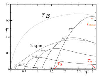
Figure 2: Transmission rates for the two-qubit channel as a function of $\tau$. The free evolution of the channel is driven by the Hamiltonian in Eq. (14), in which we set $J=1/4$. Continuous and dashed lines indicate the quantum transmission rate respectively for a standard, and a two-spin qubit encoding. The various continuous lines are for different numbers $n$ of Bob’s intermediate swaps after each Alice’s and Bob’s simultaneous swap. For reference we also plot the rate $r_{E}$ associated to the entanglement-assisted quantum transmission for the standard encoding (dotted line), which, analogously to Eq. (13), can be computed by $r_{E}\equiv{Q_{E}(\eta)}/{\tau}$, with $Q_{E}(\eta)$ being the entanglement-assisted capacity of a single amplitude damping channel vittorio05 , i.e. $Q_{E}(\eta)=(1/2)\max_{p\in[0,1]}{H_{2}(p)+H_{2}(\eta p)-H_{2}\big{(}(1-\eta)p\big{)}}$.

$$\displaystyle\sum_{j_{1}\ldots j_{m}=0}^{1} \bar{\beta}_{1}^{j_{m}}\ldots\bar{\beta}_{n}^{j_{1}}|j_{m}\ldots j_{1}\rangle_{A}\otimes|\psi_{m+1}0\rangle_{C}$$ (10)

$$\otimes\,|\tilde{\psi}_{1}^{(j_{1})}\ldots\tilde{\psi}_{m}^{(j_{m})}\rangle_{B}$$

where $\bar{\beta}_{k}=\beta_{k}\;\gamma_{11}(\tau)$, and

$$|\tilde{\psi}_{k}^{(j_{k})}\rangle=\left\{\begin{array}[]{ll}|0\rangle&\textrm{if}\quad j_{k}=1\\ |\psi^{{}^{\prime}}_{k}\rangle\equiv\alpha_{k}|0\rangle+\beta_{k}\gamma_{12}(\tau)|1\rangle&\textrm{if}\quad j_{k}=0\end{array}\;,\right.$$

with $\gamma_{11}(\tau)$ and $\gamma_{12}(\tau)$ defined as in Eq. (6) and satisfying the constraint $|\gamma_{11}(\tau)|^{2}+|\gamma_{12}(\tau)|^{2}=1$. We notice that, at each time after having applied the two SWAP operations, the chain is always disentangled from Alice and Bob memories (see Eq. (10)). This permits to express Eq. (9) as a product of $m$ amplitude damping channels NIELSEN ; bose03 ; vittorio05 $\mathcal{D}_{\eta}$, with quantum efficiency $\eta=|\gamma_{12}(\tau)|^{2}$ equal to the transfer probability of one excitation from the first to the second spin of the chain. Indeed, neglecting a phase shift component that can always be compensated by Bob through a local operation on $B$, one has

$$\rho_{B}(m) = \bigotimes_{k=1}^{m}\left(|\bar{\beta}_{k}|^{2}\,|0\rangle\langle 0|+|\psi_{k}^{{}^{\prime}}\rangle\langle\psi_{k}^{{}^{\prime}}|\right)$$

$$= \bigotimes_{k=1}^{m}\mathcal{D}_{\eta}\left(|\psi_{k}\rangle_{A_{k}}\langle\psi_{k}|\right)=\mathcal{D}_{\eta}^{\otimes m}\left(|\Psi\rangle_{A}\langle\Psi|\right)\;.$$

Exploiting the linearity of Eq. (9) this identity can then be generalized to all (non necessarily separable) input states $|\Psi\rangle_{A}$.

The transmission rate (3) associated with the protocol in Eq. (III.1) can be now easily computed by considering the quantum channel capacity SHOR of the memoryless channel map ${\cal D}_{\eta}$. This has been derived in Ref. vittorio05 : it is null for $\eta\leqslant 0.5$ and equal to

$$Q(\eta)=\max_{p\in[0,1]}\left\{H_{2}(\eta p)-H_{2}\left((1-\eta)p\right)\right\}$$ (12)

otherwise (here $H_{2}(x)=-x\log_{2}x-(1-x)\log_{2}(1-x)$ is the binary entropy function). Equation (12) gives the maximum number of qubits which can be reliably transmitted per use of the channel ${\cal D}_{\eta}$ in the asymptotic limit of $m\gg 1$ uses. Considering that in a time interval ${T}=m\,\tau$ the protocol (9) accounts for $m$ uses of the ${\cal D}_{\eta}$, we can estimate its rate as follows:

$$r\equiv\lim_{m\to\infty}\frac{m\;Q(\eta)}{m\,\tau}=\frac{Q(\eta)}{\tau}\,.$$ (13)

It should be stressed that the possibility of achieving the rate (13) relays on the identification of an optimal encoding space SHOR which, in the general case, requires infinitely many uses of the map ${\cal D}_{\eta}$ (i.e. infinitely long transmission time). In this respect Eq. (13) should be considered more as an indication of the efficiency of the protocol (9) rather than a realistic communication rate of the chain.

In order to provide an explicit expression for the rates (13), we consider the $\hat{S}_{z}$-preserving spin chain Hamiltonian of the form

$$\hat{\mathcal{H}}=\hbar\;J(\hat{\sigma}^{x}_{1}\hat{\sigma}^{x}_{2}+\hat{\sigma}^{y}_{1}\hat{\sigma}^{y}_{2})+\hbar\;\Delta\hat{\sigma}^{z}_{1}\hat{\sigma}^{z}_{2}\;,$$ (14)

for which the excitation transfer amplitude is just a sinusoidal periodic function of $\tau$ of period $\pi/(2J)$, i.e.

$$\eta=|\gamma_{12}(\tau)|^{2}=\sin^{2}(2J\,\tau)\;.$$ (15)

For $\tau={\tau_{*}}\equiv\pi/(4J)$ the free evolution operates a SWAP between the spins, thus achieving perfect transmission of a generic quantum state. Correspondingly in this case the quantum capacity (12) of the channel is optimal and equal to one while the rate (13) is $1/{\tau_{*}}$. Given the periodicity of Eq. (15), for $\tau>{\tau_{*}}$ the rate (13) can never be higher than this quantity. However, there exists a value $\tau_{\mathrm{max}}<{\tau_{*}}$ such that $r(\tau_{\mathrm{max}})>r({\tau_{*}})$ (see Fig. 2): i.e. ${\tau_{*}}$ is not the optimal time transfer for the plain scheme (9). Notice also that the quantum capacity of the amplitude damping channel is strictly zero for $\eta\leqslant\eta_{c}=0.5$, thus meaning that for $\tau\leqslant\tau_{0}\equiv\pi/8J$, the channel does not transmit any quantum information.

In order to reduce the time $\tau_{0}$, a slightly different version of the protocol can be implemented, in which we suppose that Bob has at his disposal $n$ additional memories for each qubit that Alice sends. The protocol goes on exactly as before, except that, after each double swap, (performed from both Alice and Bob) Bob runs $n$ additional SWAP operations at regular time intervals $\tau$. The unitary transformation in Eq. (III.1) then modifies into:

$$\hat{\mathcal{W}}_{m} = \big{[}\hat{S}_{B}(m_{n})\hat{U}\cdots\hat{S}_{B}(m_{1})\hat{U}\big{]}\,\hat{S}_{A}(m)\,\hat{U}\cdots$$ (16)

$$\cdots\big{[}\hat{S}_{B}(2_{n})\hat{U}\cdots\hat{S}_{B}(2_{1})\hat{U}\big{]}\,\hat{S}_{A}(2)\,\hat{U}\cdot$$

$$\cdot\big{[}\hat{S}_{B}(1_{n})\hat{U}\cdots\hat{S}_{B}(1_{1})\hat{U}\big{]}\,\hat{S}_{A}(1)\;.$$

In this way Bob can enhance the transfer fidelity vgdaniel , at the price that both time and memory requirements are increased by a factor $n$ for each qubit sent by Alice. The capacity of such a channel can be evaluated exactly as before, except that the quantum efficiency $\eta$ is now dependent of $n$, and it is given by:

$$\eta_{n}\equiv\sum_{k=0}^{n}|\gamma_{11}(\tau)|^{2k}|\gamma_{12}(\tau)|^{2}=1-(1-\eta)^{n+1}\;,$$ (17)

where $\eta=|\gamma_{12}(\tau)|^{2}$ is the quantum efficiency for $n=0$. In Fig. 2 we plotted the corresponding quantum transmission rates as a function of the time between two successive swaps $\tau$ for different values of $n$. Notice that the time $\tau_{0}$ is reduced, as one increases $n$.

III.2 Exploiting the internal dynamics of the chain

In this section we show how memory effects induced by the free evolution of the chain can be exploited in order to simplify encoding and decoding procedures. In particular, differently from the cases discussed in the previous section, the schemes analyzed here allow one to achieve optimal transmission rate by encoding the information in only a finite number of memory elements.

The simplest version of these new classes of protocols is a variation of the “dual-rail encoding” of Ref. daniel05 . The idea is to assume that Alice uses her first two memory qubits (i.e. $A_{1}$ and $A_{2}$) to codify a single information qubit $|\psi\rangle=\alpha|0\rangle+\beta|1\rangle$, while keeping the third memory element into the reference state $|0\rangle_{A_{3}}$, i.e. following the notation of Eq. (4)

$$|\psi\rangle \rightarrow \alpha|010\rangle_{A}+\beta|001\rangle_{A}\;.$$

As in the plain scheme, every $\tau$ seconds Alice and Bob are then required to perform a sequence of SWAPs gates between their memories and the chain. In this case however, we will show that after the second SWAP by Bob (i.e. after the third SWAP by Alice) a simple magnetization measurement on their memories allow both the communicating parties to establish, independently, whether the state $|\psi\rangle$ has been exactly transmitted to Bob, or it has returned to Alice’s memory. Indeed, assume that at $t=0$ the global system is in the state

$$\big{(}\alpha|010\rangle_{A}+\beta|001\rangle_{A}\big{)}\otimes|00\rangle_{C}\otimes|00\rangle_{B}\;.$$ (18)

After the first two SWAPs of Bob and the first three SWAPs of Alice (i.e. after $2\tau$ seconds from the beginning of the transmission), it is transformed into a superposition where with probability $|\gamma_{11}(\tau)|^{2}$ the information has been returned into $A$ (encoded in $A_{3}A_{2}$), while with probability $|\gamma_{12}(\tau)|^{2}$ the information has been moved into $B$ (encoded in $B_{1}B_{2}$), i.e.

$$\gamma_{11}(\tau)\;\big{(}\,\alpha|100\rangle_{A}+\beta|010\rangle_{A}\,\big{)}\otimes|00\rangle_{C}\otimes|00\rangle_{B}$$ (19)

$$+\;\gamma_{12}(\tau)\;|000\rangle_{A}\otimes|00\rangle_{C}\otimes\big{(}\,\alpha|10\rangle_{B}+\beta|01\rangle_{B}\,\big{)}\;.$$

These two possibilities can be distinguished by Alice and Bob by performing independent magnetization measurements on their respective memories $B$ and $A$. For instance, the first possibility (i.e. information in $A$) will yield, respectively, the outcome $0$ (null total magnetization of $B$) and $1/2$ (a single spin up in $A$) for Bob and Alice measurements. Analogously, when the information is in $B$ the measurements will yield, respectively, the outcome $1/2$ and $0$. In the latter case the communicating parties can proceed by sending another qubit (encoded by Alice in $A_{6}A_{5}A_{4}$ and received by Bob in $B_{3}B_{4}$), while in the former case, first the information is (locally) moved back from $A_{3}A_{2}$ into $A_{2}A_{1}$ and the protocol is repeated until Bob is certain to receive the state. The iteration of this procedure is trivial.

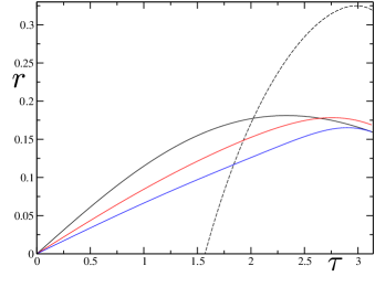
Figure 3: Quantum transmission rates for a two-qubit channel driven by the Hamiltonian in Eq. (14) with $J=1/4$ for different qubit encodings: standard encoding (one spin per qubit, dashed black line), one qubit in two spins (black line), two excitations in three spins (red line), three excitations in four spins (blue line).

To compute the transmission rate of this communication scheme we note that the probability that Bob will receive Alice’s state $|\psi\rangle$ exactly at the $j$-th iteration of the protocol is $P_{j}=|\gamma_{12}(\tau)|^{2}\;(1-|\gamma_{12}(\tau)|^{2})^{j-1}$. The average time required to transfer the qubit is then:

$$T=\sum_{j=1}^{+\infty}2\tau jP_{j}=\frac{2\tau}{|\gamma_{12}(\tau)|^{2}}\;,$$ (20)

from which we get

$$r=\frac{1}{T}=\frac{|\gamma_{12}(\tau)|^{2}}{2\tau}\;.$$ (21)

Assuming that the transferring spin chain $C$ is described by the Hamiltonian in Eq. (14), this expression has been plotted in Fig. 2 (dashed line) for a comparison with the protocols of the previous section. Notice that, for $\tau\leqslant\tau_{0}$, contrary to the standard plain encoding, the transmission rate is not zero; the maximal transfer rate however is achieved with a standard encoding.

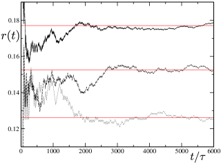
Figure 4: Instantaneous quantum transmission rates for a two-qubit channel described by the Hamiltonian in Eq. (14) with $J=1/4$ for $\tau=2$. The various curves correspond to different qubit encodings: one qubit in two spins (continuous line), two excitations in three spins (dashed line), three excitations in four spins (dotted line). Straight red lines correspond to the rates obtained after averaging over an infinite time, which are evaluated analytically from Eqs. (22), (23) and similar.

Alice and Bob can use slightly more complicated types of encodings, in order to optimize the transfer rate. For instance Alice can fix the number $E$ of excitations she employs to codify her input qubit messages in $\mathcal{N}$ spins of $A$. The case discussed before corresponds to $E=1,\>\mathcal{N}=2$; the generalization to a generic number of spins, with $E=1$ fixed, is trivial: Alice can send a number $\log_{2}(\mathcal{N})$ of qubits, provided she employs $\mathcal{N}+1$ memories (the extra memory play the same role of $A_{3}$ in the simple version of the scheme). The protocol then proceeds exactly as before, where Bob swaps on his $\mathcal{N}$-states memory. He then has to measure the magnetization at every time interval $\mathcal{N}\tau$. The success probabilities $P_{j}$ are the same as before, while the transfer rate is then given by:

$$r=\frac{|\gamma_{12}(\tau)|^{2}\;\log_{2}\mathcal{N}}{\mathcal{N}\tau}\;.$$ (22)

The case $E=2$ is slightly more complicated by the fact that, after a time $\mathcal{N}\tau$, Bob can measure two excitations with probability $|\gamma_{12}(\tau)|^{4}$ (in that case he has perfectly received the state), no excitations with probability $|\gamma_{11}(\tau)|^{4}$ (the state has perfectly returned to Alice, therefore they have to restart the protocol), or one excitation. In this last case, only one excitation is returned to Alice and she has then to retransmit it, by using the same procedure for $E=1$ described before. It can be shown that the transfer rate for the case $E=2$ is given by:

$$r=\frac{\log_{2}{\mathcal{N}\choose 2}}{\mathcal{N}\tau}\cdot\frac{(1-|\gamma_{11}(\tau)|^{4})^{2}}{1-|\gamma_{11}(\tau)|^{4}+2|\gamma_{11}(\tau)|^{2}-2|\gamma_{11}(\tau)|^{6}}\,.$$ (23)

Similar expressions for the transfer rate with higher $E$ can be obtained. The only difference is that an increasing number of possibilities appears: after a time $\mathcal{N}\tau$, Bob can receive a number of excitations $E_{B}\leqslant E$, consequently a number $E_{A}=E-E_{B}$ of excitations return to Alice. According to the value of $E_{A}$, she then has to apply a sub-protocol for the transfer of $E_{A}$ excitations, with $E_{A}\leqslant E$. This procedure has to be iterated until $E_{B}=E$.

In Fig. 3 we show the theoretical values of the transmission rates in a two-qubit channel for different values of $E$ and $\mathcal{N}$, as a function of the time $\tau$ (continuous lines); the asymptotic rate for the standard encoding, Eq. (13), is also shown for reference. Moreover we have explicitly simulated these types of communication protocols between Alice and Bob with a standard Monte Carlo numerical technique. To this end, an instantaneous transmission rate $r({t})$ can be defined as the ratio between the number of transmitted qubits $M$ until time ${t}$ and the actual transmission time ${t}$. The value of $M$ has been evaluated stochastically, following the theoretical probability distributions $P_{j}$ of the state transfer. In Fig. 4 we explicitly show the dependence of such computed instantaneous transmission rate as a function of the elapsed time $t$, for different types of encodings; notice that, by definition of transmission rate (3), the instantaneous transfer rate $r({t})$ correctly converges to the asymptotic value given by Eqs. (22), (23) and similar (straight red lines).

IV Dual-rail channel

In the previous section we analyzed the simplest spin chain model ($N=2$). The results we obtained were indicative of the possibility of exploiting memory effects to devise better communication procedures (e.g. having simpler encoding and decoding protocols). These results also showed that transmission rates could easily be computed also in the presence of such effects. In this section we would like to derive a lower bound for the maximum achievable transmission rate that can be reached in the case of an arbitrarily long spin chain. This is not a simple task MEMORY ; MEMORY1 , due to the presence of the memory correlations in the evolution of the spins chain. The point is that, at present, given a single spin chain of $N>2$ elements, we do not have communication schemes which permit Alice and Bob to verify independently that the transferring of a signal succeeded, allowing, on one hand, to move to the transmission of the next one, while, on the other hand, determining the average qubit transmission time $T$. A simple way to address these issues, is to consider the case in which the channel $C$ is composed by three identical uncoupled spin $1/2$ chains, each of them governed by an Hamiltonian $\hat{\mathcal{H}}$ that conserves the total magnetization.

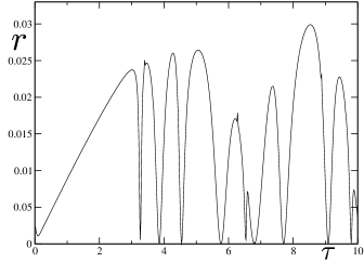
Figure 5: Quantum transmission rates as a function of $\tau$ for a dual-rail channel with classical feed-back side line for a chain of $N=8$ spins. Free evolution of the chains is governed by an Heisenberg chain with $J=1/4$. Data have been obtained numerically by truncating the series in Eq. (32) at $k_{max}=10^{5}$.

As before, we suppose that Alice has access to the leftmost spin of each of the three chains, while Bob can manipulate the spin at the opposite end of the chains. We also assume that, at time $t=0$, all the chains are set up in the ferromagnetic ground state $\left|{\bf 0}\right\rangle^{(i)}\equiv|0_{1}\ldots 0_{N}\rangle^{(i)}$ (where $i=\{1,2,3\}$ is the index that labels the chain). The communication strategy we want to analyze is the following. Alice use the chains $1$ and $2$ to transfer her first message to Bob by means of a dual-rail encoding daniel05 . Since this is a “conclusive” strategy, it allows Bob to know exactly at what instant Alice’s message has been loaded in his memory. When this happens, he will use the third chain to signal back to Alice that he is ready to receive a new qubit of information (e.g. he does so by sending a spin up message to Alice). The whole procedure is then reiterated for the transmission of the second Alice’s message.

To see how this works in details let us first consider a simplified version of the above scheme, where the feed-back message by Bob is transmitted to Alice through a side classical communication line (e.g. a telephone line). In this case we need only to consider the information transfer along the spin chains $1$ and $2$ from Alice to Bob. Assume that the first message Alice wants to transmit is the qubit $\left|\psi\right\rangle=\alpha|0\rangle+\beta\left|1\right\rangle$. The chains $1$ and $2$ are then prepared into the following superposition:

$$\left|{\bf s}(1)\right\rangle\equiv\alpha\left|{\bf 0}\right\rangle^{(1)}\otimes\left|{\bf 1}\right\rangle^{(2)}+\beta\left|{\bf 1}\right\rangle^{(1)}\otimes\left|{\bf 0}\right\rangle^{(2)}\,.$$ (24)

The system is then let freely evolve, such that the excitation in Eq. (24) will propagate along the two chains:

$$\left|{\bf s}(1)\right\rangle\stackrel{{\scriptstyle\hat{U}(\tau)}}{{\longrightarrow}}\sum_{n=1}^{N}\gamma_{1n}(\tau)\left|{\bf s}(n)\right\rangle,$$ (25)

where $\gamma_{ij}(\tau)$ is the same as in Eq. (6). Following Ref. daniel05 , at regular time intervals $\tau$ Bob performs a magnetization measurement on the last spins of the chain $1$ and $2$, in order to check if the state $\left|\psi\right\rangle$ has traveled to him. In the meantime Alice does nothing and waits until she receives Bob’s “OK” feed-back message on the phone. At the first Bob’s measurement, which happens after a time $\tau$, if he measures a non-zero magnetization, he concludes that the qubit $\left|\psi\right\rangle$ is located on the last spins of the chain: therefore he can safely SWAP it into his memory $B$. According to Eq. (25), such event happens with probability $\pi_{1}\equiv|\gamma_{1N}(\tau)|^{2}$. In this case he communicates to Alice via the classical channel the success of information transfer, and she will proceed by sending another qubit through the chains $1$ and $2$ following the same procedure.

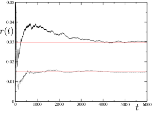
Figure 6: Instantaneous quantum transmission rates for a dual-rail channel with $N=8$ spins, for $\tau=8.5$; $J=1/4$. Black curves shows the results of a Monte Carlo simulation of the protocol, straight red lines indicate the theoretical values of the rate, obtained after averaging over an infinite time. Upper curves correspond to the case in which the transmission protocol is assisted from a backward classical communication channel; in the lower curves backward communication from Bob to Alice occurs via a single quantum spin chain, equal to the two forward communicating ones.

Vice-versa, if the first outcome of Bob’s measurement is zero, then he knows that the system has been projected in the state

$$\frac{1}{\sqrt{1-\pi_{1}}}\sum_{n=1}^{N-1}\gamma_{1n}(\tau)|{\bf s}(n)\rangle\;,$$ (26)

where Alice’s qubit of information $|\psi\rangle$ is still contained in the chains $1$ and $2$. Bob has then another possibility to receive the state $\left|\psi\right\rangle$: he can wait for another time $\tau$, before performing the second magnetization measurement. Just before the measurement, the system will be in the state:

$$\frac{1}{\sqrt{1-\pi_{1}}}\sum_{n=1}^{N}\Big{(}\gamma_{1n}(2\tau)-\gamma_{Nn}(\tau)\gamma_{1N}(\tau)\Big{)}|{\bf s}(n)\rangle\;.$$ (27)

Correspondingly Bob’s probability to receive the qubit at the second measurement is then:

$$\pi_{2}=\frac{1}{\pi_{1}}|\gamma_{1N}(2\tau)-\gamma_{NN}(\tau)\gamma_{1N}(\tau)|^{2}\;.$$ (28)

If the transfer has been still unsuccessful, then he can repeat this strategy, until he is sure the state has been transferred. After each time $k\tau$ he has a probability $\pi_{k}$ to receive the state that can be obtained by simply iterating this scheme:

$$\pi_{k}=\left[\prod_{j=1}^{k-1}\frac{1}{1-\pi_{j}}\right]\cdot|c_{k}|^{2}\;,$$ (29)

where

$$c_{k}=\gamma_{1N}(k\tau)-\sum_{j=1}^{k-1}\gamma_{NN}(j\tau)\>c_{k-j}\;.$$ (30)

The probability of having $k-1$ failures and a success at the $k$-th measurement is thus expressed by:

$$P(k) = \pi_{k}\cdot(1-\pi_{k-1})\cdot(1-\pi_{k-2})\cdot\ldots\cdot(1-\pi_{1})$$ (31)

$$= \bigg{|}\gamma_{1N}(k\tau)-\sum_{j=1}^{k-1}\gamma_{NN}(j\tau)\>c_{k-j}\bigg{|}^{2}\;.$$

The total probability of success after $k$ steps is given by the sum of all $P(j)$, with $j=1,\ldots,k$. It can be shown that, under a very general hypothesis on the system Hamiltonian $\hat{\mathcal{H}}$, the probability of success converges to 1 in the limit $k\to\infty$ daniel05B .

By knowing all the probabilities (31) it is possible to evaluate the average time $T$ needed for the transfer of the first qubit from Alice to Bob. Indeed, since $P(k)$ is exactly the transfer probability after $k$ steps, and since each step takes $\tau$ seconds, we get

$$T=\sum_{k=1}^{+\infty}k\,\tau\,P(k)\;.$$ (32)

If we suppose that Bob can instantaneously communicate to Alice the fact that he effectively received the qubit (for example via a classical communication channel), and that, immediately after having known the transfer success, she sends another qubit, we than obtain the transfer rate $r=1/T$. In Fig. 5 we plot this quantity for a dual rail channel composed of two identical isotropic spin $1/2$ Heisenberg chains of the form $\hat{\mathcal{H}}=-\hbar\;J\;\sum_{j=1}^{N}\,\hat{{\vec{\sigma}}}_{j}^{(i)}\,\hat{{\vec{\sigma}}}_{j+1}^{(i)}$ for which the amplitudes $\gamma_{ij}(\tau)$ have been explicitly computed in Ref. bose03 . As discussed at the beginning of the section, the requirement of a classical communication channel needed as a feedback from Bob to Alice can be relaxed, provided that there is a third spin chain connecting them. In this case, when Bob has received the qubit, he puts an excitation in this chain. Alice then uses the same protocol for the forward communication in order to receive it. If the third chain is identical to the others, the average time required for the forward and the backward communication are equal, therefore the rate for the quantum communication halves.

In Fig. 6 we show the results of a Monte Carlo simulation of these dual-rail protocols: the instantaneous transmission rates as a function of time in units of $\tau$ are plotted. We simulated both the case assisted with a backward classical communication channel (upper curves), and the case in which backward communication from Bob to Alice occurs via a third quantum spin chain, equal to the two forward communicating ones (lower curves).

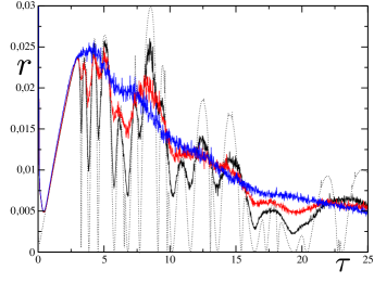
Figure 7: Quantum transmission rates for a dual-rail channel with $N=8$ spins, as a function of $\tau$. The various continuous curves are for different values of the random tilting time: $\epsilon=0.01$ (black), 0.02 (red), 0.04 (blue curve). The dashed black line corresponds to the case of no tilting time ($\epsilon=0$). A truncation value of $k_{\mathrm{max}}=5000$ has been adopted here.

Finally we notice that, if the elapsed time between two successive Bob’s measurements $\tau$ is kept fixed, the transmission rate $r$ as a function of $\tau$ displays a highly non monotonic behavior, which is typically unpredictable. In particular there are some values of $\tau$ for which the transmission rate suddenly drops to a value close to zero. This is due to the sinusoidal quasi-periodic behavior of the amplitudes $\gamma$. A possible strategy in order to reduce these singularities, would be that of randomly varying the time interval between measurements, i.e. $\tau+\delta\tau$ (where $\delta\tau$ is randomly chosen in $(-\epsilon,\epsilon)$, and $\epsilon$ indicates the strength of the tilting time). Numerical results are shown in Fig. 7, where the various curves refer to different values of $\epsilon$. For small times $\tau$ the rate is independent of $\epsilon$, while at long times its behavior approaches that of a power law $r\sim\tau^{-1}$.

V Conclusions

We have analyzed spin-chain communication protocols in which a single quantum channel is used in order to admit multiple-qubit transfer in time between two distant parties. Without using Hamiltonians engineered ad hoc, or complex encoding and decoding operations, Bob is generally not able to perfectly recover Alice’s information, due to the dispersive free evolution of the chain. Moreover, memory effects naturally arise in these types of protocols: part of the information previously injected by Alice into the chain typically interferes with subsequent data sent. Nevertheless in some cases we are able to evaluate the transmission rates even in presence of such memory effects. In the case of a two-spin channel, despite the fact that the chain can act as a simple swapper, thus making it possible to obtain a perfect state transfer from Alice to Bob, we showed that the maximum achievable transfer rate is not obtained in correspondence of perfect transfer. Transmission rates along arbitrary long chains can be analyzed numerically in the framework of the dual-rail protocol, thus permitting to establish a lower bound for the maximum achievable rate.

- (1) M.A. Nielsen and I.L. Chuang, Quantum Computation and Quantum Information (Cambridge University Press, England, 2000).
- (2) S.C. Benjamin and S. Bose, Phys. Rev. Lett. 90, 247901 (2003); M.H. Yung, D.W. Leung, and S. Bose, Quant. Inform. Comput. 4, 174 (2004).
- (3) J. Fitzsimons and J. Twamley, Eprint: quant-ph/0601120.
- (4) G. De Chiara, R. Fazio, C. Macchiavello, S. Montangero, and G.M. Palma, Phys. Rev. A 70, 062308 (2004); ibidem, 72, 012328 (2004); Q. Chen, J. Cheng, K.-L. Wang, and J. Du, Eprint: quant-ph/0510147.
- (5) S. Bose, Phys. Rev. Lett 91, 207901 (2003).
- (6) T.J. Osborne and N. Linden, Phys. Rev. A 69, 052315 (2004).
- (7) H.L. Haselgrove, Phys. Rev. A 72, 062326 (2005).
- (8) A.Wójcik,T. Łuczak, P. Kurzyński, A. Grudka, T. Gdala, and M. Bednarska, Phys. Rev. A 72, 034303 (2005).
- (9) V. Giovannetti and R. Fazio, Phys. Rev. A 71, 032314 (2005).
- (10) D. Burgarth and S. Bose, Phys. Rev. A 71, 052315 (2005).
- (11) D. Burgarth, V. Giovannetti, and S. Bose, J. Phys. A: Math. Gen. 38, 6793 (2005).
- (12) D. Burgarth and S. Bose, New J. Phys. 7, 135 (2005).
- (13) V. Giovannetti and D. Burgarth, Phys. Rev. Lett., 96, 030501 (2006).
- (14) J. He, Q. Chen, L. Ding, and S.-L. Wan, Eprint: quant-ph/0606088.
- (15) D. Burgarth and S. Bose, Phys. Rev. A 73, 062321 (2006); J.-M. Cai, Z.-W. Zhou, and G.-C. Guo, Eprint: quant-ph/0603228.
- (16) M. Christandl, N. Datta, A. Ekert, and A.J. Landahl, Phys. Rev. Lett. 92, 187902 (2004); C. Albanese, M. Christandl, N. Datta, and A. Ekert, Phys. Rev. Lett. 93, 230502 (2004); M. Christandl, N. Datta, T. C. Dorlas, A. Ekert, A. Kay, and A.J. Landahl, Phys. Rev. A 71, 032312 (2004).
- (17) G.M. Nikolopoulos, D. Petrosyan, and P. Lambropoulos, J. Phys.: Condens. Matter 16, 4991 (2004); Europhys. Lett. 65, 297 (2004).
- (18) M.H. Yung and S. Bose, Phys. Rev. A 71, 032310 (2005).
- (19) M. Paternostro, G.M. Palma, M.S. Kim, and G. Falci, Phys. Rev. A 71, 042311 (2005).
- (20) P. Karbach and J. Stolze, Phys. Rev. A 72, 030301(R) (2005).
- (21) M.B. Plenio and F.L. Semião, New J. Phys. 7, 73 (2005); M.J. Hartmann, M.E. Reuter, and M.B. Plenio, New J. Phys. 8, 94 (2006); Y. Li, T. Shi, B. Chen, Z. Song, and C.P. Sun, Phys. Rev. A 71, 022301 (2005); T. Shi, Y. Li, Z. Song, and C.P. Sun, Phys. Rev. A 71, 032309 (2005); Z. Song and C.P. Sun, Fizika Nizkikh Temperatur 31, 8 (2005) – Eprint: quant-ph/0412183.
- (22) V. Srinivasa, J. Levy, and C.S. Hellberg, Eprint: quant-ph/0606089.
- (23) F. de Pasquale, G. Giorgi, and S. Paganelli, Phys. Rev. Lett. 93, 120502 (2004).
- (24) A. Romito, C. Bruder, and R. Fazio, Phys. Rev. B 71, 100501 (2005); A. Lyakhov and C. Bruder, New J. Phys. 7, 181 (2005).
- (25) I. D’Amico, Eprint: cond-mat/0511470.
- (26) E. Jané, G. Vidal, W. Dür, P. Zoller, and J.I. Cirac, Quantum Inf. and Comp. 3, 15 (2003); L.-M. Duan, E. Demler, and M.D. Lukin, Phys. Rev. Lett. 91, 090402 (2003).
- (27) M.J. Hartmann, F.G.S.L. Brandão, and M.B. Plenio, Eprint: quant-ph/0606097; D. Angelakis, M.F. Santos, and S. Bose, Eprint: quant-ph/0606159.
- (28) C. Macchiavello and G.M. Palma, Phys. Rev. A 65, 050301(R) (2005); G. Bowen and S. Mancini, Phys. Rev. A 69, 012306 (2004); D. Kretschmann and R.F. Werner, Phys. Rev. A 72, 062323 (2005).
- (29) V. Giovannetti, J. Phys. A: Math. Gen. 38, 10989 (2005).
- (30) Simultaneity between Alice and Bob operations and the assumption of having uniform time intervals are not fundamental in our analysis: these hypotheses are considered only to simplify the problem and to compact the notation.
- (31) C.H. Bennett and P.W. Shor, IEEE Trans. Inf. Theory 44, 2724 (1998).