The Quantum Cocktail Party

Abstract

We consider the problem of decorrelating states of coupled quantum systems. The decorrelation can be seen as separation of quantum signals, in analogy to the classical problem of signal-separation rising in the so-called cocktail-party context. The separation of signals cannot be achieved perfectly, and we analyse the optimal decorrelation map in terms of added noise in the local separated states. Analytical results can be obtained both in the case of two-level quantum systems and for Gaussian states of harmonic oscillators.

In its digital form, information is perfectly copy-able and broadcastable at will. In its analog form of everyday life, however, information often comes mixed-up. This is the case, for example, when we join a cocktail party, and we hear two people speaking simultaneously: their voices come together in one signal to our ears. Our brain is easily able to ”tune” to one voice and ignore the other, and, sometimes to even grasp both of them. If, however, we want to digitalise the two speeches separately, we need to de-mix the two voices, and this is generally a hard task for a neural-network software, a problem which is indeed commonly known as the cocktail party problem cock . In Quantum Mechanics we have a similar situation for the quantum information. We known that quantum information cannot be copied or broadcast exactly, due to the no-cloning theorem Wootters82 (which asserts the impossibility of making exact copies of an unknown quantum state drawn from a non orthogonal set). Such a limitation is actually very valuable for quantum cryptography, as it forbids an eavesdropper from creating copies of a transmitted quantum cryptographic key. In the presence of noise, however, (i. e. when transmitting ”mixed” states), it can happen that we are able to increase the number of copies of the same state if we start with sufficiently many identical originals. Indeed, it is even possible to purify in such broadcasting process—the so-called super-broadcasting our . Clearly, the increased number of copies cannot augment the available information about the original input state, and this is actually due to the fact that the final copies are not statistically independent, and the correlations between them influence the extractable information estcor . It is now natural to ask if we can remove such correlations and make them independent again, a process which is a quantum analog of the cocktail party problem. Clearly, such quantum un-mixing or de-correlating cannot be done exactly, otherwise we would increase the information on the state. However, we will show here that we can achieve perfect de-correlation at expense of some more noise in each copy.

In the typical cocktail party scenario we have two microphones in the same room at different locations. If we denote the amplitude of a sound wave emitted by two people by $\alpha(t)$, $\beta(t)$ respectively, then microphones will in general record a linear combination of this messages (for simplification, we neglect the possible delays in the time arrival to different receivers from different sources):

$$x(t) =C_{11}\alpha(t)+C_{12}\beta(t)$$ (1)

$$y(t) =C_{21}\alpha(t)+C_{22}\beta(t)$$ (2)

where $C_{ij}$ are parameters which depend on the microphone sensitivities and on their distance from the speakers, and $x(t)$, $y(t)$ are the recorded signals. Amazingly, even if the parameters $C_{ij}$ are unknown and signals $\alpha(t)$, $\beta(t)$ do not have any distinctive feature (e.g. different frequency band), the separation of original signals is still possible, under the sole assumption that original signals where uncorrelated (and the additional technical assumption that the probability distributions of the signals amplitude at different times were not Gaussian). A way to achieve the un-mixing task is by the so called independent component analysis (ICA), which uses the fact that the probability distribution of a sum of independent random variables is ”more Gaussian” than the probability distribution of the variables themselves. This strategy is sometimes called the blind independent component analysis, as we know neither the signal probability distribution nor the mixing parameters $C_{ij}$. After a successful application of the above strategy one is left with independent signals $\alpha^{\prime}(t)$ and $\beta^{\prime}(t)$, which in the ideal case differ from the input signals $\alpha(t)$ and $\beta(t)$ by a scaling factor (in reality there is always some noise), and are uncorrelated. Mathematically the de-correlation task can be stated in term of factorization of the conditional probability distributions as follows

$$p_{AB}(\alpha^{\prime},\beta^{\prime}|\alpha,\beta)=p_{A}(\alpha^{\prime}|\alpha)p_{B}(\beta^{\prime}|\beta).$$ (3)

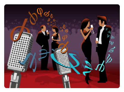
Figure 1: When we join a cocktail party and we hear two people speaking simultaneously, their voices come together in a single signal to our ears (which we can simulate by two microphones). If we want to digitalise the two speeches separately, we then need to de-mix the two voices, and this is generally a hard task for a neural-network software, a problem which is indeed commonly known as the cocktail party problem. In Quantum Mechanics we can also consider a situation of de-correlating two signals, but in this case the signals are not classical, and are encoded using quantum states. [Picture courtesy by Tomasz Szkodziński].

A quantum strict analog of the problem can be formulated as follows. Assume we have a bipartite quantum system (e.g. two qubits, two quantum modes of electromagnetic field, etc.) initially in a state $|0\rangle\otimes|0\rangle$ (or more generally in some mixed state $\rho_{AB}$). The signal is encoded using unitary operations $U_{A}(t)$, $U_{B}(t)$ acting locally at time $t$ on subsystems $A$ and $B$, respectively. The communication of quantum signals will amount to sending the states $[U_{A}(t)\otimes U_{B}(t)]|0\rangle\otimes|0\rangle$ at different times $t$, each time rotated by a different pair of unitary matrices $U_{A}(t)$ and $U_{B}(t)$, depending on the quantum message intended to be transmitted. After this encoding, the system passes through the environment which causes the two signals to be mixed in analogy to classical mixing of signals in microphones. This mixing can be represented by a unitary operation $V$ that entangles both qubits with the environment state $|E\rangle$ as follows

$$|\psi(t)\rangle_{ABE}=V(U_{A}(t)\otimes U_{B}(t)\otimes I)|0\rangle\otimes|0\rangle\otimes|E\rangle.$$ (4)

The analog of the classical cocktail-party problem would be now to determine the “signals” $U_{A}(t)$ and $U_{B}(t)$—or the state $[U_{A}(t)\otimes U_{B}(t)]|0\rangle\otimes|0\rangle$—from the output state of $AB$ only, without even knowing the interaction with the environment $V$: this would be a strict quantum analog of blind independent component separation. In this sense we would de-correlate the signals $U_{A}(t)$ and $U_{B}(t)$. This quantum version of the cocktail-party problem is much harder than its classical counterpart, for many reasons, including the no-cloning theorem, which forbids to determine the output state from a single copy: an approximate solution, if possible, would need at least some additional assumptions about the time self-correlation of each separate signal, along with the aid of a quantum memory to store the whole time-sequence of output states of $AB$ and a full joint measurement on the whole sequence.

We pose here a simpler, but a closely related problem of de-correlating two quantum signals, in the scenario where the signals $U_{A}$, $U_{B}$ are encoded on a correlated state $\rho_{AB}$ as: $U_{A}\otimes U_{B}\rho_{AB}U^{\dagger}_{A}\otimes U^{\dagger}_{B}$, but no additional mixing operation $V$ is applied. We want to de-correlate the received state, and the desired result is two completely uncorrelated systems $A$ and $B$, each one in a state that carries information about the signals $U_{A}$ and $U_{B}$, respectively.

Therefore, according to the above scenario, let $\rho_{AB}$ be a density matrix of two (generally correlated) quantum systems. The hardest case will be when the two systems $A$ and $B$ are identical, and the state $\rho_{AB}$ doesn’t change under permutation of them. The information is encoded on the state $\rho_{AB}$ via the local unitary transformations as follows

$$\rho_{AB}(\alpha,\beta)\doteq U_{A}(\alpha)\otimes U_{B}(\beta)\rho_{AB}U_{A}^{\dagger}(\alpha)\otimes U_{B}^{\dagger}(\beta),$$ (5)

$\alpha$ and $\beta$ denoting random variables. The de-correlating quantum transformation ${\mathscr{D}}$ we are seeking should act as follows:

$$\rho_{AB}(\alpha,\beta)\longrightarrow\tilde{\rho}_{A}(\alpha)\otimes\tilde{\rho}_{B}(\beta)$$ (6)

with $\tilde{\rho}_{A}(\alpha)\doteq U_{A}(\alpha)\tilde{\rho}_{A}U_{A}^{\dagger}(\alpha)$, and $\tilde{\rho}_{B}(\beta)\doteq U_{B}(\beta)\tilde{\rho}_{B}U_{B}^{\dagger}(\beta)$. This means that the map acts covariantly with respect to the action of $U_{A}(\alpha)\otimes U_{B}(\beta)$. The output state is uncorrelated, and we want the matrices $\tilde{\rho}_{A}(\alpha)$ and $\tilde{\rho}_{B}(\beta)$ to contain as little noise as possible, namely they will carry the same signal, but possibly with higher noise. In other words, we want the states $\tilde{\rho}_{A}(\alpha)$ and $\tilde{\rho}_{B}(\beta)$ to be as close as possible to the input marginal states $\rho_{A}(\alpha)=\textrm{Tr}_{B}[\rho_{AB}(\alpha,\beta)]$, $\rho_{B}(\beta)=\textrm{Tr}_{A}[\rho_{AB}(\alpha,\beta)]$, respectively.

At the output the two classical signals $\alpha$ and $\beta$ encoded on the joint state $\rho_{AB}(\alpha,\beta)$ are recovered by separate identical measurements on systems $A$ and $B$, yielding the probability distribution

$$p_{AB}(\alpha^{\prime},\beta^{\prime}|\alpha,\beta)=\textrm{Tr}[\Pi(\alpha^{\prime})\otimes\Pi(\beta^{\prime})\rho_{AB}(\alpha,\beta)],$$ (7)

where $\Pi(\alpha)$ and $\Pi(\beta)$ are positive operators describing the local measurements on $A$ and $B$, fulfilling the normalization condition $\int\textrm{d}\alpha^{\prime}\Pi(\alpha^{\prime})=\int\textrm{d}\beta^{\prime}\Pi(\beta^{\prime})=\openone$.

If instead we first apply the de-correlation operation ${\mathscr{D}}$, and then perform the measurements we get the probability distribution

$$\begin{split}p^{\mathscr{D}}_{AB}(\alpha^{\prime},\beta^{\prime}|\alpha,\beta)=&\textrm{Tr}[\Pi(\alpha^{\prime})\otimes\Pi(\beta^{\prime})\tilde{\rho}_{A}(\alpha)\otimes\tilde{\rho}_{B}(\beta)]\\ =&p_{A}(\alpha^{\prime}|\alpha)p_{B}(\beta^{\prime}|\beta),\end{split}$$ (8)

achieving the solution of the cocktail party problem as in Eq. (3). We want to stress that the de-correlated probabilities $p_{A}(\alpha^{\prime}|\alpha)$ and $p_{B}(\beta^{\prime}|\beta)$ will be generally more noisy than the respective marginals of the original joint probability (indeed a perfect de-correlation is not possible, since it would violate linearity of quantum mechanical evolutions: see also Refs. Terno ; Mor ).

Now we will show how de-correlation can be achieved in two specific examples: on qubits, and on qumodes (the so-called continuous variables, i. e. quantum harmonic oscillators).

Consider a couple of qubits. For qubits the state is conveniently described in the Bloch form. The information $(\alpha,\beta)$ is encoded by $U_{A}(\alpha)$ and $U_{A}(\beta)$ on the direction of the Bloch vectors $\boldsymbol{n}_{A}(\alpha)$ and $\boldsymbol{n}_{B}(\beta)$ of the marginal states

$$\begin{split}\rho_{A}(\alpha)=&\textrm{Tr}_{B}[\rho_{AB}(\alpha,\beta)]=\tfrac{1}{2}(\openone+\eta\boldsymbol{n}_{A}(\alpha)\cdot\boldsymbol{\sigma}),\\ \rho_{B}(\beta)=&\textrm{Tr}_{A}[\rho_{AB}(\alpha,\beta)]=\tfrac{1}{2}(\openone+\eta\boldsymbol{n}_{B}(\beta)\cdot\boldsymbol{\sigma}),\end{split}$$ (9)

where $\boldsymbol{\sigma}=(\sigma_{x},\sigma_{y},\sigma_{z})$ is the vector of Pauli matrices $\sigma_{\alpha}$. Covariance of the de-correlation map means that the direction of the Bloch vectors $\boldsymbol{n}_{A}(\alpha)$ and $\boldsymbol{n}_{B}(\beta)$ should be preserved in the output states, i. e.

$$\begin{split}&\tilde{\rho}_{A}(\alpha)=\frac{1}{2}(\openone+\eta^{\prime}\boldsymbol{n}_{A}(\alpha)\cdot\boldsymbol{\sigma}),\\ &\tilde{\rho}_{B}(\beta)=\frac{1}{2}(\openone+\eta^{\prime}\boldsymbol{n}_{B}(\beta)\cdot\boldsymbol{\sigma}),\end{split}$$ (10)

namely only the length of the Bloch vector (i. e. the purity of the state) is changed $\eta\to\eta^{\prime}$. The fact the output states are more noisy corresponds to a reduced length of the Bloch vector $\eta^{\prime}<\eta$. The directions of the Bloch vectors $\boldsymbol{n}_{A}(\alpha)$ and $\boldsymbol{n}_{A}(\beta)$ are completely arbitrary. The optimal de-correlation map will maximize the length $\eta^{\prime}$ of the Bloch vector, namely it will produce the highest purity of de-correlated states. It can be shown that the general form of a two-qubit channel ${\mathscr{D}}$ covariant under $U_{A}(\alpha)\otimes U_{B}(\beta)$ and invariant under permutations of the two qubits can be parameterized with three positive parameters only (effectively two due to normalization)

$${\mathscr{D}}(\rho_{AB})=a\rho_{AB}+b{\mathscr{D}}_{1}(\rho_{AB})+c{\mathscr{D}}_{2}(\rho_{A}B),$$ (11)

where ${\mathscr{D}}_{1}$ and ${\mathscr{D}}_{2}$ are given by

$${\mathscr{D}}_{1}(\rho_{AB})= \tfrac{1}{3}\left(\openone\otimes\rho_{B}+\rho_{A}\otimes\openone-\rho_{AB}\right)$$ (12)

$${\mathscr{D}}_{2}(\rho_{AB})= \tfrac{1}{9}\left(4\openone\otimes\openone+\rho_{AB}-2\openone\otimes\rho_{B}-2\rho_{A}\otimes\openone\right)$$ (13)

and the trace preserving condition gives $a+b+c=1$. This is a very restricted set of operations, which is due to the fact that the covariance condition is very strong. As a consequence a generic joint state $\rho_{AB}$ cannot be de-correlated (of course, apart from the trivial de-correlation to a maximally mixed state), and the states for which de-correlation is possible have the form

$$\rho_{AB}=\tfrac{1}{4}\left[\openone\otimes\openone+\kappa(\sigma_{z}\otimes\openone+\openone\otimes\sigma_{z})+\lambda\sigma_{z}\otimes\sigma_{z}\right].$$ (14)

We emphasize that for a generic state $\rho_{AB}$ one can reduce correlations, but only for states of the form (14) the correlations can be completely removed. The noise of the de-correlated states depends on parameters $\kappa$ and $\lambda$ as depicted in Figure 2.

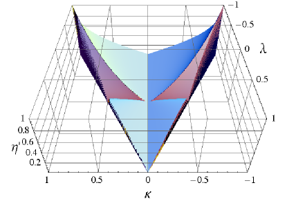
Figure 2: Length $\eta^{\prime}$ of the Bloch vectors of the de-correlated states of two qubits starting from the joint state in Eq. (14). The 3D plot depicts the maximal achievable $\eta^{\prime}$ versus the parameters $\kappa$ and $\lambda$ of the input state.

We consider now the case of de-correlation for qumodes. For a couple of qumodes in a joint state $\rho_{AB}$ the information $(\alpha,\beta)$ (with $\alpha$ and $\beta$ complex) is encoded as follows

$$D(\alpha)\otimes D(\beta)\rho_{AB}D(\alpha)^{\dagger}\otimes D(\beta)^{\dagger},$$ (15)

$D(z)=\exp(za^{\dagger}-z^{*}a)$ for $z\in{\mathbb{C}}$ denoting a single-mode displacement operator, $a$ and $a^{\dagger}$ being the annihilation and creation operators of the mode. In particular, it can be shown that it is always possible to de-correlate any joint state of the form (15), with $\rho_{AB}$ representing a two-mode Gaussian state, namely

$$\rho_{AB}=\frac{1}{\pi^{4}}\int d^{4}\boldsymbol{q}\,e^{-\frac{1}{2}\boldsymbol{q}^{T}\boldsymbol{M}\boldsymbol{q}}D(\boldsymbol{q})\;,$$ (16)

where $\boldsymbol{M}$ is the $4\times 4$ (real, symmetric, and positive) correlation matrix of the state, $\boldsymbol{q}=(q_{1},q_{2},q_{3},q_{4})$, and $D(\boldsymbol{q})=D(q_{1}+iq_{2})\otimes D(q_{3}+iq_{4})$. The de-correlation channel covariant under $D(\alpha)\otimes D(\beta)$ is given by

$${\mathscr{D}}(\rho)=\frac{\sqrt{\hbox{det}\boldsymbol{G}}}{(2\pi)^{2}}\int d^{4}\boldsymbol{x}\,e^{-\frac{1}{2}\boldsymbol{x}^{T}\boldsymbol{G}\boldsymbol{x}}D(\boldsymbol{x})\rho D^{\dagger}(\boldsymbol{x}),$$ (17)

with suitable positive matrix $G$, and the resulting state ${\mathscr{D}}(\rho_{AB})$ is still Gaussian, with a new block-diagonal covariance matrix $\widetilde{\boldsymbol{M}}$, thus corresponding to a de-correlated state.

A special example of Gaussian state of two qumodes is the so-called twin beam, which can be generated in a quantum optical lab by parametric down-conversion of vacuum. In this case $\boldsymbol{M}$ is given by

$$\boldsymbol{M}=\frac{1+\lambda^{2}}{1-\lambda^{2}}\openone-\frac{2\lambda}{1-\lambda^{2}}\left(\begin{array}[]{cc}0&\sigma_{z}\\ \sigma_{z}&0\end{array}\right)\;,$$ (20)

with $0\leq\lambda<1$. The map (17) with

$$\boldsymbol{G}=\frac{2\lambda}{1-\lambda^{2}}\left[\openone+\left(\begin{array}[]{cc}\varepsilon&\sigma_{z}\\ \sigma_{z}&\varepsilon\end{array}\right)\right]\;,$$ (23)

and arbitrary $\varepsilon>0$, provides two de-correlated states with $\widetilde{\boldsymbol{M}}=(\frac{1+\lambda}{1-\lambda}+\varepsilon)\openone$, which correspond to two thermal states with mean photon number $\bar{n}=\frac{\lambda}{1-\lambda}+\frac{\varepsilon}{2}$ each.

The striking difference between the qubit and the qumode cases is that for qubits only few states can be de-correlated, whereas for qumodes any joint Gaussian state can be de-correlated. This is due to the fact that the covariance group for qubits comprises all local unitary transformations, whereas for qumodes includes only local displacements, which is a very small subset of all possible local unitary transformations in infinite dimension. Indeed, for the same reason de-correlation becomes much easier when considering covariance with respect to unitary transformations of the form $U\otimes U$ (i. e. with the same information encoded on the quantum systems, e. g. the qubit Bloch vectors have the same direction, or the qumodes are displaced in the same direction), which is actually the case when considering broadcasted states. Covariant de-correlation of this kind for multiple copies gives insight into the problem of how much individual information can be preserved, while all correlations between copies are removed.

- (1) Unsupervised Adaptive Filtering, Volume 1: Blind Source Separation, ed. by Simon Haykin (John Wiley & Sons, New York, 2000).
- (2) W. K. Wootters and W. H. Zurek, Nature 299, 802 (1982).
- (3) G. M. D’Ariano, C. Macchiavello, and P. Perinotti, Phys. Rev. Lett. 95, 060503 (2005).
- (4) R. Demkowicz-Dobrzanski, Phys. Rev. A 71, 062321 (2005).
- (5) D. R. Terno, Phys. Rev. A 59, 3320 (1999).
- (6) T. Mor, Phys. Rev. Lett. 83, 1451 (1999).